Galerkin Methods for Boltzmann-Poisson transport with reflection conditions on rough boundaries
2The University of Texas at Austin - Institute for Computational Engineering and Sciences & Department of Mathematics)
Abstract
We consider in this paper the mathematical and numerical modelling of
reflective boundary conditions (BC) associated to Boltzmann - Poisson systems, including diffusive reflection in addition to specularity, in the context of electron transport in semiconductor device modelling at nano scales, and their implementation in Discontinuous Galerkin (DG) schemes.
We study these BC on the physical boundaries of the device and develop a numerical approximation to model an insulating boundary condition, or equivalently,
a pointwise zero flux mathematical condition for the electron transport equation.
Such condition balances
the incident and reflective momentum flux at the microscopic level,
pointwise at the boundary, in the case of a more general mixed reflection with momentum dependant specularity probability .
We compare the computational prediction of physical observables
given by the numerical implementation of these different reflection conditions in our DG scheme for BP models, and
observe that the diffusive condition influences the kinetic moments over the whole domain in position space.
Keywords: Galerkin; Boltzmann-Poisson; boundary; reflection; diffusive; specular.
1 Introduction
The dynamics of electronic transport in modern semiconductor devices can be described by the semiclassical Boltzmann-Poisson (BP) model
| (1.1) |
| (1.2) |
where
is the probability density function (pdf) over phase space of a carrier in the -th energy band in position ,
with crystal momentum at time . The collision operators model
-th and -th carrier recombinations, collisions with phonons or generation effects. is the electric field,
is the electric potential,
is the -th energy band surface, the -th charge density is the k-average of , is the electric charge of the -th carrier,
is the doping profile, and is the electric permittivity of the material.
The BP model for electron transport on a single conduction energy band for electrons has the form
| (1.3) |
| (1.4) |
with the quantum mechanical electron group velocity , and the electron density . The collision integral operator describes the scattering over the electrons, where several mechanisms of quantum nature can be taken into account. In the low density regime, the collisional integral operator can be approximated as linear in , having the form
| (1.5) |
where is the scattering kernel, representing non-local interactions of electrons with a background density distribution. For example, in the case of silicon, one of the most important collision mechanisms are electron-phonon scatterings due to lattice vibrations of the crystal, which are modeled by acoustic (assumed elastic) and optical (non-elastic) non-polar modes, the latter with a single frequency , given by
| (1.6) | |||||
with , constants for silicon. The symbol indicates the usual Dirac delta distribution corresponding to the well known Fermi’s Golden Rule [13]. The constant is related to the phonon occupation factor
where is the Boltzmann constant and is the lattice temperature.
The semi-classical Boltzmann description of electron transport in semiconductors is, for a truly 3-D
device, an equation in six dimensions plus time when the device is not in steady state.
The heavy computational cost is the main reason why the BP system had been
traditionally solved numerically by means of Direct Simulation Monte Carlo (DSMC) methods
[14]. However, after the pioneer work [15], in recent years,
deterministic solvers to the BP system were proposed in
[16, 17, 18, 19, 20, 21, 22].
These methods provide accurate results which, in general, agree well with those obtained from Monte
Carlo (DSMC) simulations, often at a fractional computational time. Moreover, these type of solvers can resolve
transient details for the electron probability density function , which are
difficult to compute with DSMC simulators.
The initial methods proposed in [18, 19, 20, 21] using weighted essentially non-oscillatory (WENO) finite
difference schemes to solve the Boltzmann-Poisson system, had the advantage that the scheme is relatively simple to code and very stable even on coarse meshes for solutions containing sharp
gradient regions. However, a disadvantage of the WENO methods is that it requires smooth meshes to achieve high order accuracy, hence it is not very flexible for adaptive meshes.
Motivated by the easy hp-adaptivity and the simple communication pattern of
the discontinuous Galerkin (DG) methods for macroscopic (fluid level) models [23, 24, 25, 26], it was proposed in [27, 28] to implement a DG
solver to the full Boltzmann equation, that is capable of capturing transients of the probability
density function.
In the previous work [27, 28], the first DG solver for
(1.1)-(1.2) was proposed, and some numerical calculations were shown for one and
two-dimensional devices. In [29], the DG-LDG scheme for the Boltzmann-Poisson
system was carefully formulated, and extensive numerical studies were performed to validate the
calculations. Such scheme
models electron transport along the conduction band for 1D diodes and 2D double gate MOSFET devices
with an analytic Kane energy band model.
A DG method for full conduction bands BP models was proposed
in [30], following the lines of the schemes in [27, 28, 29],
generalizing the solver that uses the Kane non-parabolic band and adapting it to treat the full energy band case. A preliminary benchmark of numerical results shows that the direct evaluation of the Dirac delta function can be avoided, and so an accurate high-order simulation with comparable computational cost to the analytic band
cases is possible. It would be more difficult or even unpractical to produce the full band computation with other
transport scheme. It is worth to notice that a high-order positivity-preserving DG
scheme for linear Vlasov-Boltzmann transport equations, under the action of quadratically confined
electrostatic potentials, independent of the electron distribution, has been developed in
[31]. The authors there show that these DG schemes conserve mass and preserve the positivity of the solution without
sacrificing accuracy. In addition, the standard semi-discrete schemes
were studied showing stability and error estimates.
The type of DG method discussed in this paper, as was
done in [29], belongs to a class of
finite element methods originally devised to solve hyperbolic conservation laws containing only
first order spatial derivatives, e.g. [32, 33, 34, 35, 36]. Using a piecewise
polynomial space for both the test and trial functions in the spatial variables, and coupled with
explicit and nonlinearly stable high order Runge-Kutta time discretization, the DG method is a
conservative scheme that has the advantage of flexibility for arbitrarily unstructured meshes, with
a compact stencil, and with the ability to easily accommodate arbitrary hp-adaptivity. For
more details about DG scheme for convection dominated problems, we refer to the review paper
[37], later generalized to the Local DG (LDG) method to solve the
convection diffusion equations [38] and elliptic equations [39].
Regarding Boundary Conditions (BC), there are several kinds of BC for BP semiconductor models. They vary according to the considered device and physical situation. We list below several examples of BC that could arise in the case of electron transport along a single conduction band.
Charge neutrality boundary conditions, given by [4]
| (1.7) |
where is the position domain. This BC is imposed in source and drain boundaries, where electric currents enter or exit the device, to achieve neutral charges there, as .
Reflective BC happen in insulating boundaries, usually defined by a Neumann boundary , of 2D and 3D devices. In general, reflective BC can be formulated as the values of the pdf at the inflow boundary being dependent on the outflow boundary values
| (1.8) |
denoting that the reflection boundary condition is a function of the outflow boundary values of the probability density function, where the Neumann Inflow Boundary is defined as
| (1.9) |
| (1.10) |
with the momentum domain, outward unit normal, and the Neumann Outflow Boundary is defined as
| (1.11) |
Specular Reflection BC over the Neumann Inflow Boundary is given by
| (1.12) |
| (1.13) |
Diffusive reflection is a known condition from kinetic theory, in which the distribution function at the Inflow boundary is proportional to a Maxwellian [1], [2] with the temperature at the wall
| (1.14) |
| (1.15) |
Mixed reflection BC models the effect of a physical surface on electron transport in metals and semiconductors, giving the reflected pdf representing the electrons as a linear convex combination of specular and diffuse components, as in the formula
is sometimes called specularity parameter. It can either be constant or a function, dependant of the momentum. For example, the work by Soffer [5] studies a statistical model for the reflection from a rough surface in electrical conduction. It derives a specularity parameter which depends on the momentum, given by
| (1.17) |
where is the rms height of the rough interface, and
is th angle between the incident electron and the interface surface normal.
Reflection BC is a widely studied topic
in the context of the kinetic theory of gases
modelled by Boltzmann Equations.
However, in the context of kinetic models for electron transport in semiconductors,
there is less extensive previous work related
to the study of the effect of reflection boundary conditions such
as diffusive, specular, or mixed reflection.
An example of the list of references where reflection BC are studied for Boltzmann equations in the context of kinetic theory of gases
would include the works of
Cercignani [3] and Sone [1],
where the specular, diffusive, and mixed reflection BC
are formulated for the Boltzmann Eq. for gases.
V. D. Borman, S. Yu. Krylov, A. V. Chayanov [9]
study the nonequilibrium phenomena at a gas-solid interface.
The recent paper of Brull, Charrier, Mieussens [10]
studies the gas-surface interaction at a nano-scale and the boundary conditions for the associated Boltzmann equation. The recent work of
Struchtrup [11] studies as well the
Maxwell boundary condition and velocity dependent accommodation
coefficients in the context of gases mentioned.
It considers the convex combination of specular reflection, isotropic scattering, and diffusive reflection, incorporating
velocity dependent coefficients into a Maxwell-type reflection kernel. It develops a modification of Maxwell’s BC, extending the Maxwell model by allowing it to incorporate velocity dependent accomodation coefficients into the microscopic description
and satisfying conditions of reciprocity and unitary probability normalization.
Regarding reflectivity in the context of Boltzmann models of electron transport,
Fuchs [6] proposed a boundary condition for the probability density function of free electrons incident in the material surface, which is a convex combination of specular & diffuse reflection with a constant specularity parameter . Greene ([7], [8]) studied conditions for the Fuchs BC in which the specularity parameter is dependant on the angle of the momentum , deriving a boundary condition for electron distributions at crystal surfaces valid for metal, semimetal, & semiconductor surfaces, and showing that Fuchs’ reflectivity parameter differs from the kinetic specularity parameter in physical significance and in magnitude. It considers
the unperturbed electron states of a crystal with an ideal perfectly specular surface as standing wave states, and
the diffusive reflection killing partially the incoming wave function.
Soffer [5] studies a statistical model for the electrical conduction, and derives under certain assumptions, such as
a rough surface random model with a Gaussian probability
of height above or below a horizontal plane,
analytical formulas for a momentum dependant specularity parameter associated to this physical phenomena, abovementioned in (1.17).
As mentioned before, is the rms height of rough interface, and
is th angle between the incident electron and the interface surface normal.
The reference book of
Markowich, Ringhofer, & Schmeiser [12]
for semiconductor equations
discusses the mathematical definition of boundaries according
to the physical phenomena, and defines accordingly the kind
of BC to be imposed at those boundaries: Dirichlet, Neumann, Inflow and Outflow boundaries.
A work of particular importance for us is the one by
Cercignani, Gamba, and Levermore [4].
They study high field approximations to a Boltzmann-Poisson system and boundary conditions in a semiconductor. The BP system for electrons in a semiconductor in the case of high fields and small devices is considered. Boundary conditions are proposed at the kinetic level that yield charge neutrality at ohmic contacts, which are Dirichlet boundaries, and at insulating Neumann boundaries.
Both BC, either the one yielding charge neutrality at Dirichlet boundaries, or the one rendering zero flux of electrons at the boundary, assume that the pdf is proportional to a ground state
associated to an asymptotic expansion of a dimensionless Boltzmann-Poisson system. Then they study closures of moment equations and BC for both the pdf and for the moment closures.
The paper [40] also comments on the study of boundary conditions for kinetic and macroscopic approximations for the Boltzmann - Poisson system in bounded domains. Jüngel mentions in his semiconductors book [2]
the different kinds of reflection BC common on the
kinetic theory of gases, specular, diffusive, and mixed reflection
but no further study of diffusive and mixed reflection BC in the context of semiconductors is pursued.
We intend to present in this work a mathematical, numerical, and computational study of the effect of diffusive, specular, and mixed reflection BC in Boltzmann-Poisson models of electron transport in semiconductors, solved by means of Discontinuous Galerkin FEM solvers. We study the mathematical formulation of these reflection BC in the context of BP models for semiconductors, and derive equivalent numerical formulations of the diffusive and mixed reflection BC with non-constant , such that an equivalent numerical zero flux condition is satisfied pointwise at the insulating Neumann boundaries at the numerical level. We present numerical simulations for a 2D silicon diode and a 2D double gated MOSFET, comparing the effects of specular, diffusive, and mixed reflection boundary conditions in the physical observable quantities obtained from the simulations.
2 BP system with coordinate transformation assuming a Kane Energy Band
The Kane Energy Band Model is a dispersion relation between the conduction energy band (measured from a local minimum) and the norm of the electron wave vector , given by the analytical function ( is a constant parameter, is the electron reduced mass for Si, and is Planck’s constant)
| (2.18) |
For our preliminary numerical studies we will use a Boltzmann-Poisson model as in [29] , in which the conduction energy band is assumed to be given by a Kane model. We use the following dimensionalized variables, with the related characteristic parameters
A transformed Boltzmann transport equation is used as in [29] as well, where the coordinates used to describe are: , the cosine of the polar angle, the azimuthal angle , and the dimensionless Kane Energy , which is assumed as the conduction energy band. We will assume that the wall temperature is equal to the lattice temperature, so , and . So , where
| (2.19) |
A new unknown function is used in the transformed Boltzmann Eq. [29] , which is proportional to the Jacobian of the transformation and to the density of states (up to a constant factor)
where
| (2.20) |
The transformed Boltzmann transport equation for used in [29] is
| (2.21) |
The vector represent the 2D cartesian components of the electron velocity , in the coordinate system (, , ). The triplet represent the transport in the phase space of the new momentum coordinates (, , ) due to the self consistent electric field
with
and the orthonormal vector basis in our momentum coordinate space.
The right hand side of (2.21) is the collision operator (having applied the Dirac Delta’s due to electron-phonon scattering, which depend on the energy differences between transitions)
with the dimensionless parameters
The electron density is
where
| (2.22) |
Hence, the dimensionless Poisson equation is
| (2.23) |
with
3 Discontinuous Galerkin Method for Transformed Boltzmann - Poisson System and Implementation of Boundary Conditions
The domain of the devices to be considered can be represented by means of a rectangular grid in both position and momentum space. This rectangular grid, bidimensional in position space and tridimensional in momentum space, is defined as
where , , , , ,
The finite dimensional space used to approximate the functions is the space of piecewise continuous polynomials which are piecewise linear in and piecewise constant in ,
| (3.24) |
with the set
of tensor product polynomials, linear over the element
, and constant over the element
.
The function will denote the piecewise polynomial approximation of over elements ,
The density on the cell is, under this approximation,
3.1 DG Formulation for Transformed Boltzmann Equation
The Discontinuous Galerkin formulation for the Boltzmann equation (2.21) is as follows. Find , s.t.
| (3.25) | |||||
for any test function . In (3.25), the boundary integrals are given by
where the upwind numerical fluxes are defined as
| (3.26) |
3.2 Poisson Equation - Local Discontinuous Galerkin (LDG) Method
By means of this scheme we find a solution , where and , the set of linear polynomials on . It involves rewriting the equation into the form
| (3.27) |
where is a known function that can be computed at each time step once is solved from (3.25), and the coefficient depends on . The Poisson system is only on the domain. Hence, we use the grid , with , , where denotes the oxide-silicon region, and the grid in is consistent with the five-dimensional rectangular grid for the Boltzmann equation in the silicon region. The approximation space is defined as
| (3.28) |
Here denotes the set of all polynomials of degree at most on . The LDG scheme for (3.27) is: to find , such that
| (3.29) | |||||
hold true for any . In the above formulation, we choose the flux as follows, in the -direction, we use , . In the -direction, we use , . On some part of the domain boundary, the above flux needs to be changed to accommodate various boundary conditions. For example, in the case of a double gate MOSFET device, for the boundary condition of the Poisson equation, at source, at drain and at gate. For the rest of the boundary regions, we have homogeneous Neumann boundary conditions, i.e., . The relative dielectric constant in the oxide-silicon region is , in the silicon region is . Near the drain then, we are given Dirichlet boundary condition, so we need to flip the flux in direction: let and if the point is at the drain. For the gate, we need to flip the flux in direction: let and , if the point is at the gate. For the bottom, we need to use the Neumann condition, and flip the flux in y-direction, i.e., , . This scheme described above will enforce the continuity of and across the interface of silicon and oxide-silicon interface. The solution of (3.2) gives us approximations to both the potential and the electric field , .
3.3 RK-DG Algorithm for BP, from to
The following RK-DG algorithm for BP is a dynamic extension of the Gummel iteration map. We write below the steps to evolve from time to time .
-
1.
Compute the electron density .
-
2.
Solve Poisson Eq. for the given by Local DG, obtaining the potential and the electric field . Compute then the respective transport terms .
-
3.
Solve by DG the advection and collision part of the Boltzmann Equation. A Method of Lines (an ODE system) for the time dependent coefficients of (degrees of freedom) is obtained.
-
4.
Evolve ODE system by Runge-Kutta from to . (If partial time step necessary, repeat Step 1 to 3 as needed).
4 Boundary Conditions Implementation for 2D-, 3D- devices at Boundaries
We will consider in this work 2D devices in position space,
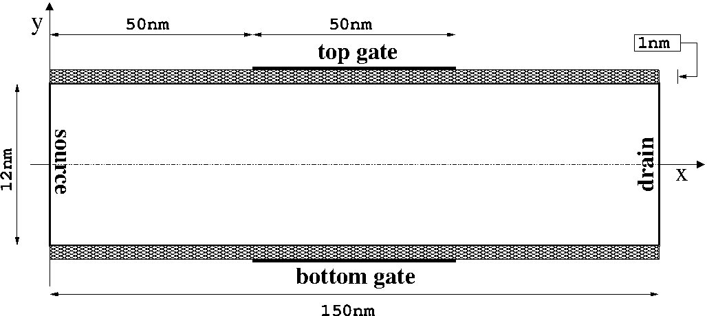
which need a 3D momentum description for kinetic equations modeling semiconductors. For example, a common device of interest is a 2D double gate MOSFET. A schematic plot of it is given in Figure 4.1. The shadowed region denotes the oxide-silicon region, whereas the rest is the silicon region. Potential bias are applied at the source, drain, and gates. The problem is symmetric about the x-axis.
Another possible 2D problem is the case of a bi-dimensional bulk silicon diode, for which the doping is constant all over the physical domain, and which would have just an applied potential (bias) between the source and the drain (no gates), with insulating reflecting boundaries at and .
We consider in the following sections the different kinds of boundary conditions for 2D devices and their numerical implementation, either at -boundaries or at -boundaries.
4.1 Poisson Equation Boundary Condition
The BC for Poisson Eq. are imposed over the -domain.
For example, for the case of a 2D Double gated MOSFET, Dirichlet BC would be imposed to the potential , as we have three different applied potentials biases, Volts at the source , Volts at the drain , Volts at the gates. Homogeneous Neumann BC would be imposed for the rest of the boundaries, that is, .
For the case of a 2D bulk silicon diode,
we impose Dirichlet BC for the difference of potential
between source and drain,
Volts at the source ,
Volts at the drain .
For the boundaries we impose Homogeneous Neumann BC too, that is, .
4.2 Charge Neutrality BC
4.3 Cut - Off BC
In the -space, we only need to apply a cut-off Boundary Condition. At , is made machine zero,
| (4.30) |
No other boundary condition is necessary for -boundaries, since analytically we have that
-
•
at , ,
-
•
at , ,
-
•
at , ,
so, at such regions, the numerical flux always vanishes.
5 Reflection BC on BP
Reflection Boundary Conditions can be expressed in the form
| (5.31) |
such that the following pointwise zero flux condition is satisfied at reflecting boundaries, so
| (5.32) | |||||
as in Cercignani, Gamba, Levermore[4], where the given BC at Neumann boundary regions at the kinetic level is such that the particle flow vanishes.
For simplicity we write . We will study three kinds of reflective boundary conditions: specular, diffusive, and mixed reflection. The last one is a convex combination of the previous two, but the convexity parameter can be either constant or momentum dependant, . We go over the mathematics and numerics related to these conditions below.
5.1 Specular Reflection
It is clear that, at the analytical level, the specular reflection BC (1.12) satisfies the zero flux condition pointwise at reflecting boundaries, since
Specular reflection BC in our transformed Boltzmann Eq. for the new coordinate system is mathematically formulated in our problem as
| (5.33) |
To impose numerically specular reflection BC at in the DG method, we follow the procedure of [29]. We relate the inflow values of the pdf, associated to the outer ghost cells, to the outflow values of the pdf, which are associated to the interior cells adjacent to the boundary, as given below by
| (5.34) | |||
In the case of the boundary , assuming , , with , if then . The values of at the related inner and outer boundary cells () and () must be equal at the boundary . Indeed
Therefore, from the equality above we find the relation between the coefficients of at inner and outer adjacent boundary cells, given by
| (5.35) |
Following an analogous procedure for the boundary , we have
Then
| (5.36) |
and hence
5.2 Diffusive Reflection
The diffusive reflection BC can be formulated as
| (5.37) |
where and are the function and parameter such that the zero flux condition is satisfied at each of the points of the Neumann Boundary, so
It follows then that
| (5.38) |
| (5.39) |
| (5.40) |
The diffusive reflection BC, formulated in terms of the unknown function of the transformed Boltzmann Equation 2.21, is expressed as
| (5.41) |
| (5.42) |
| (5.43) |
We have, over the portion of the boundary considered, that for and for . Therefore
| (5.44) |
| (5.45) |
5.2.1 Numerical Formulation of Diffusive BC for DG
For the DG numerical method, we have to project the boundary conditions to be imposed in the space . Our goal is to have at the numerical level an equivalent pointwise zero flux condition at the reflection boundary regions.
We formulate then the diffusive BC for the DG method as
where is the projector of functions into the finite element space , is a function in our piecewise polynomial space for and is a parameter such that the zero flux condition is satisfied numerically, so
In the space of piecewise continuous polynomials which are tensor products of polynomials of degree in and of degree in , it holds that
| (5.47) | |||
Therefore, for our particular case we have
| (5.48) |
so for the numerical zero flux condition pointwise we have that
We observe then that we can obtain a numerical equivalent of the pointwise zero flux condition if we define
In our particular case, in which we have chosen our function space as piecewise linear in and piecewise constant in , the projection of the Maxwellian is a piecewise constant approximation representing its average value over each momentum cell , that is
Therefore, for the particular space we have chosen, we have that
| (5.49) | |||
By the upper index in a sum we mean to say that the sum is taken over the values of for which . We notice that the polynomial approximation is equal to the analytical function operating on the polynomial approximation . However, the constant needed in order to achieve the zero flux condition numerically is not equal to the value of this parameter in the analytical solution. In this case is an approximation of the analytical value using a piecewise constant approximation of the Maxwellian (its average over cells).
The approximate operator gives a piecewise linear polynomial dependant on with time dependent coefficients. We have that
where is such that, at the boundary of the cell , it is given by
We define , so in . Then,
| (5.50) |
We summarize the main results of these calculations for and , by showing just the ones related to (the case is analogous). At the boundary , the inner cells associated to outflow have , adjacent to the boundary, whereas the ghost cells related to inflow have the index . We compute the integral as
Therefore, we have, with , below, that
Once the coefficients of have been computed, we use them to obtain the polynomial approximation , with , from (5.49)
We have at the same time, by definition, that
Therefore, the coefficients for are
| (5.51) |
| (5.52) |
| (5.53) |
keeping in mind that our parameter is given by the formula
5.3 Mixed Reflection
The mixed reflection condition is a convex combination of the specular and diffusive reflections:
is the Specularity Parameter, . can be either constant or , a function of the wave vector momentum.
For constant, it can be shown easily that the previous formulas obtained for the specular and diffusive BC, in particular the previous formulas for , works also in this case to obtain a zero flux condition at the Neumann boundaries:
However, for a function of the crystal momentum the same choice of and as in the diffusive case does not necessarily guarantee that the zero flux condition will be satisfied at Neumann boundaries. Therefore, a new condition for in order to satisfy this condition must be derived. We derive it below.
The general mixed reflection BC can be formulated as
where and are the function and parameter such that the pointwise zero flux condition is satisfied at the Neumann boundaries
Since
we conclude then that
| (5.54) |
| (5.55) |
The general mixed reflection BC then has the specific form
with s.t.
Notice that the product has the form
| (5.56) |
which for the case of constant, it reduces to the original function and parameter .
| ct, | ||||
However, for the non-constant case the new function and parameter , need to be used instead, as the previous , will not satisfy the zero flux condition in general for , since
A more general possible case of mixed reflection BC would have a specularity parameter dependent on position, momentum, and time. The related reflective BC would then be
| and | (5.57) |
where is the equilibrium probability distribution (not necessarily a Maxwellian) according to which the electrons diffusively reflect on the physical boundary. and are the functions such that the zero flux condition is satisfied pointwise at insulating boundaries
Therefore we conclude for this reflection case that
| (5.58) |
| (5.59) |
and then the full BC formula for the reflection case is
Remark: can be any iid random variable in .
5.3.1 Numerical Implementation
The numerical implementation of the general mixed reflection with specularity parameter is done in such a way that a numerical equivalent of the pointwise zero flux condition is achieved.
The general mixed reflection boundary condition in our DG numerical scheme is
We will be using the notation
| (5.61) |
The specific form of and will be deduced from the numerical analogous of the mixed reflection boundary condition. We want to satisfy numerically the zero flux condition
| (5.63) |
In the space of piecewise continuous polynomials which are tensor products of polynomials of degree in and of degree in , it holds that
| (5.64) | |||
Therefore, we have for our particular case that
Using this, our numerical pointwise zero flux condition is
We conclude then that we can achieve a numerical equivalent of the pointwise zero flux condition by defining
| (5.65) |
Therefore, the inflow BC in our DG numerical method is given by the expression
The particular form of the coefficients defining the piecewise polynomial approximation for the general mixed reflection BC is presented below for the boundary , since the calculations for the case of the boundary are analogous.
For the boundary , which defines the sign of . Outflow cells have the index . They are cells inside the domain adjacent to the boundary. Inflow cells have the index . They are ghost cells adjacent to the boundary. We have in our case that
If (inflow), (outflow), the projection integrand is given by
The coefficients of are given below. We have now that , so from the previous two formulas then
Since on one hand we have
and on the other hand
we conclude that the coefficients for are
| (5.67) |
6 Numerical Results
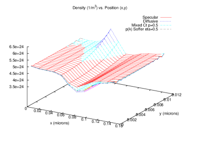
6.1 2D bulk silicon
We present results of numerical
simulations for the case of n
2D bulk silicon diode with an applied bias
between the boundaries ,
and reflection BC at the boundaries
(Figs. 6.2).
The required dimensionality in momentum space is a
3D .
The specifics of our simulations are:
Initial Condition: . Final Time: 1.0ps
Boundary Conditions (BC):
-space: Cut-off - at ,
is machine zero.
Only needed BC in : transport normal to the boundary analitically zero at ’singular points’ boundaries:
At , .
At , = 0.
At , = 0.
-space: Charge Neutrality at boundaries
.
Bias - Potential: V, V.
Neumann BC for Potential at : .
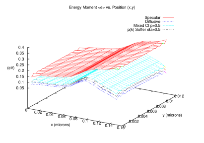
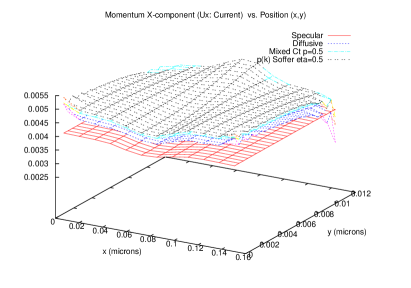
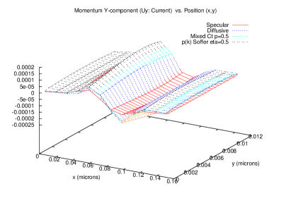
Reflection BC at : Specular, Diffusive, Mixed Reflection with constant specularity ,
and Mixed Reflection using a momentum dependent specularity , the nondimensional roughness rms height coefficient being .
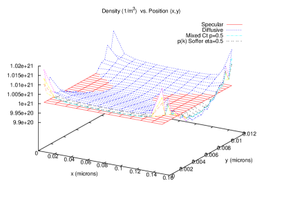
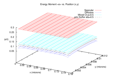
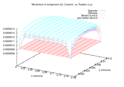
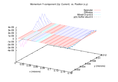
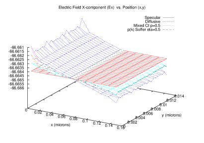
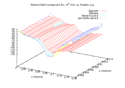
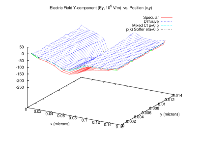
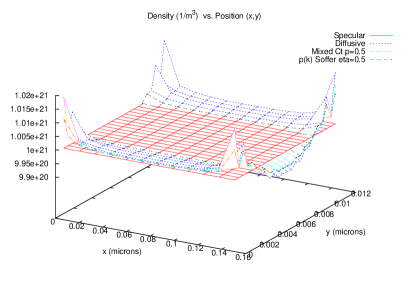
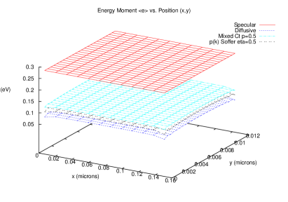
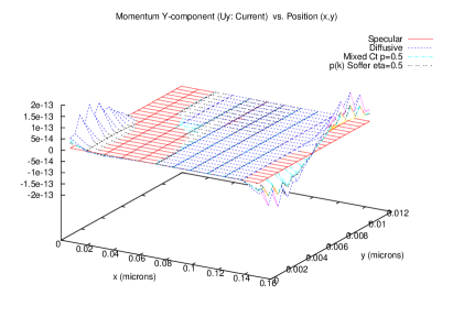
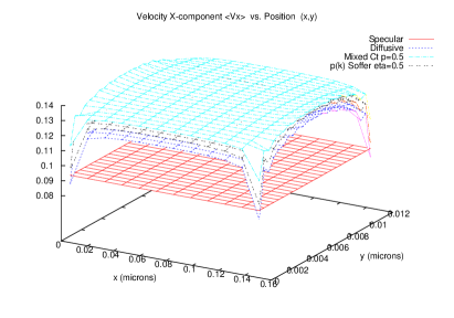
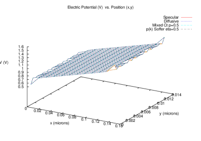
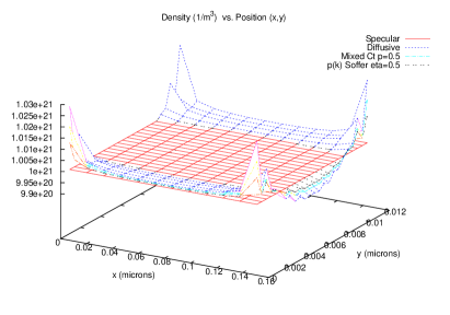
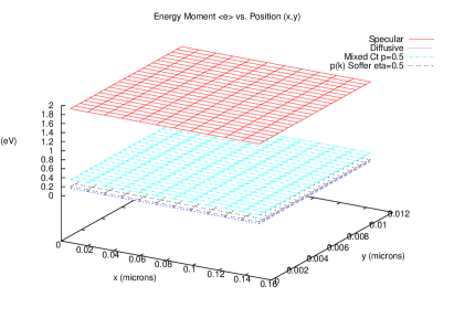
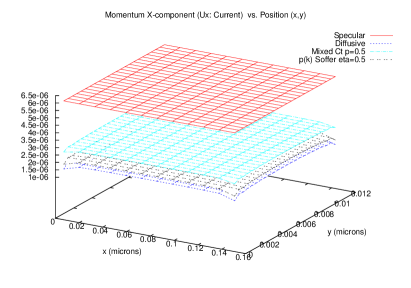
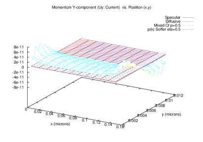
We observe an influence of the Diffusive and Mixed Reflection in macroscopic observables. It is particularly noticeable in the kinetic moments. For example, the charge density slightly increases with diffusivity close to the reflecting boundaries, and, due to mass conservation, alters the density profile over the domain. Momentum & mean velocity increase with diffusive reflection over the domain, while the energy is decreased by diffusive reflection over the domain. There is a negligible difference in the electric field component below its orders of magnitude for the different reflection cases.
6.2 2D double gated MOSFET
We present as well the results of numerical simulations for the case of a 2D double gated MOSFET device (Figs. 6.3). On one hand, the BC for the Poisson Eq. for this device would be the Dirichlet BC Volts at the source , Volts at the drain , and Volts at the gates. On the other hand, Homogeneous Neumann BC are imposed at the rest of the boundaries. Specular reflection is applied at the boundary because the solution is symmetric with respect to for our 2D double gate MOSFET (Fig. 4.1). At the boundary we apply specular, diffusive, and mixed reflection BC, both with constant , and with a momentum dependent with roughness coefficient . We use again the initial condition: , running the simulations up to the physical time of 1.0ps. We use again as well a cut-off BC in the boundary of the momentum domain, so is machine zero at , and we apply charge neutrality BC at .
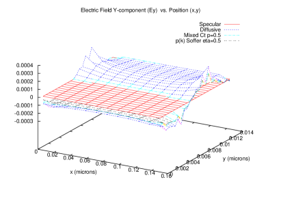
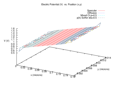
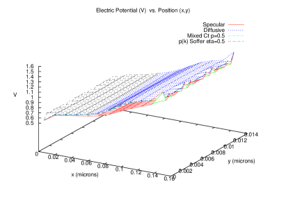
We observe a quantitative difference in the kinetic moments and other observables between the different cases of reflective BC, with the physical quantities being of the same order of magnitude. The electron density increases close to the gates with diffusive reflection, and close to the center of the device, given by the boundary , the density profile is greater for specular reflection. The energy moment clearly decreases with diffusive reflection over the physical domain. The momentum -component for specular reflection is less than for the other reflective cases. There is a difference in the profile of the electric field -component between the specular reflection and the other cases that include diffusivity, increasing it with diffusive reflection close to the drain. The electric field -component increases with diffusive reflection close to the boundary representing the center of the device. The electric potential is greater for the cases including diffusive reflection than for the perfectly specular case.
6.3 Electrons reentering the 2D domain with reflective BC in and periodic BC in : comparison of bulk silicon with collisionless plasma
We consider in this case almost the same physical situation and parameters for the previous section on the 2D bulk silicon,
except that instead of using the charge neutrality conditions we apply periodic boundary conditions in the -boundaries,
simulating then that the electrons reenter the material on the opposite -boundary after the outflow exits the domain.
We compare these simulations with ones in which no collisions are considered, corresponding the latter to the case of a collisionless
plasma with reflective BC in and periodic BC in . For both cases, bulk silicon with electron-phonon collisions and the collisionless electron gas,
we still apply an external potential such that at and Volt at . This can be understood in the framework
of periodic BC in as a periodic sawtooth wave with period equal to the length of the -domain.
We do this comparison in order to study the effect of the reflective boundary conditions in , with and without the influence of the collisions over electrons, and we let the electrons re-enter the domain under periodic boundary conditions in , eliminating then the charge neutrality conditions in and any possible effect due to the latter. Since due to the periodic BC in the electrons re-enter the domain after they exit it in outflow, the effect of boundary conditions is exclusively related to the reflection in the transport domain in the -boundaries.
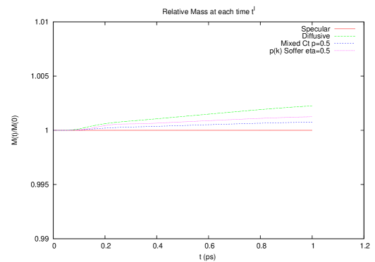
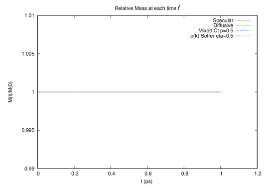
For example, in Figs. 6.6 we present the plots of Relative Mass vs Time (ps) for Specular, Diffusive, Mixed with constant and momentum dependent specularity for different sets of simulations.
The top figure is related to simulations for bulk silicon with charge neutrality conditions on the non-reflecting boundaries,
the middle figure is associated to simulations for bulk silicon with periodic boundary conditions on the non-reflecting boundaries, and the bottom figure is related to the simulations for collisionless electron transport with periodic boundary conditions on the non-reflecting boundaries.
The last two sets of simulations mentioned conserve the mass during all the time, and these sets isolate the effect of reflection boundary conditions by using periodic boundary conditions instead of charge neutrality conditions. The first set associated to charge neutrality conditions in adition to reflection boundary conditions, however, have a slight increase in the relative mass
of less than 0.5%. This slight increase then is associated only to the inclusion of charge neutrality conditions and a possible accumulation of numerical error due solely to it.
We notice in our comparison then the following effects of the collision operator in comparison with the collisionless plasma case. As expected, the main effect of collisions is to decrease the magnitude of the average energy, average velocity and momentum (therefore the current) of electrons over the domain (Fig. 6.4). The effect of collisions on the distribution of the electron density profile over the domain is negligible. Regarding the isolated effects of the reflection boundary conditions in the kinetic moments and other physical observables of interest by considering the collisionless plasma with periodic BC in , we notice, as earlier in the section for bulk silicon, the slight increase of the density profile close to the reflecting boundaries when adding diffusivity in the boundary conditions, and by conservation of mass, a decrease of the density profile over the center of the domain. The mean energy decreases over the position domain with the inclusion of diffusive reflection BC, as well as the components (which are the dominant) of the momentum and velocity (Fig. 6.5). It is important to notice this expected effect of the isolated reflection BC in the collisionless plasma case, since for the case that includes electron-phonon collisions combined with adding diffusive reflection BC gives actually an increase in the components of the momentum and velocity compared to the purely specular reflection case (Fig. 6.4). The collisionless plasma with periodic BC in and reflection BC in isolates the effect of the latter then and shows the expected behaviour of a decrease in the mean energy, velocity and momentum -compoments when adding diffusivity in the reflection boundary conditions.


7 Conclusions
We have considered the mathematical and numerical modeling of Reflective Boundary Conditions in 2D devices and their implementation in DG-BP schemes. We have studied the specular, diffusive and mixed reflection BC on the boundaries of the position domain of the device.
We developed a numerical equivalent of the zero flux condition at the position domain boundaries for the case of a more general mixed reflection with a momentum dependant specularity parameter .
We compared the influence of these different reflection cases in the computational prediction of moments
after implementing numerical BC equivalent to the respective
reflective BC, each one satisfying a mathematical zero flux condition at insulating boundaries.
There are effects due to the inclusion of diffusive reflection boundary conditions over the moments and physical observables of the probability density function, whose influence is not only restricted to the boundaries but actually to the whole domain. Particularly noticeable effects of the inclusion of diffusivity in kinetic moments are the increase of the density close to the reflecting boundary, the decrease of the mean energy over the domain and, in the case when electron-phonon collisions for silicon are included, the increase of the -components of the mean velocity and momentum over the domain, whereas for the collisionless case, for which only the effects of the reflection boundary conditions are considered (such as when electrons are allowed to reenter the material via periodic boundary conditions in ), a decrease in those -components of mean velocity and momentum is observed, as expected when adding diffusivity to the reflection boundary conditions.
To summarize, specular boundary conditions have the physical meaning of a reflection with a perfectly smooth surface with no roughness. Diffusive boundary conditions are the opposite case, with the physical meaning of a rough surface that completely diffuses the momentum. That means, for a fixed at a time , since , the probability density function is higher for momentum vectors with a lower energy band value, therefore the momentum with the highest value, for that given at time , occurs at , where the origin of the momentum space has been chosen as the position of the local energy band valley.
Hence, our physical interpretation of the diffusive reflection condition is that
it diffuses the momentum giving a higher probability for lower magnitude momentum values, with highest probability density value at .
The mixed reflection condition is a convex combination of both, meaning that the reflection process is partially specular and partially diffuses the momentum, with the probability of specularity potentially depending on the momentum variable. Estimating which boundary condition is more physical, we believe mixed reflection case may be the most suitable, as no surface is in practice perfectly specular, and the diffusive reflection is the case in the other end of the spectrum that minimizes the total reflected momentum. Regarding on how to understand the quantitative differences between the output for the considered boundary conditions, we propose, in Section 6.3, a numerical study of the different reflection conditions for collisionless electrons with periodic conditions on the other two boundaries. This case provides the best understanding of the boundary condition role in the simulation as it isolates effects of the reflection conditions, since there is no dissipation from collision mechanisms, and the electrons reenter the domain after exiting a periodic boundary. In fact, we show in Figures 6.5 that the diffusivity in the boundary condition, as expected, lowers the momentum in the main direction of transport of the electrons, which is (the transport in the direction is negligible), and it also lowers the energy average. Both of these quantitative differences are expected from the reflection of the electrons with a rough boundary. Regarding the quantitative difference between the density output, we observe that particles tend to stay closer to the rough boundaries when increasing the degree of diffusivity in the boundary condition, since the diffusivity decreases the total reflected momentum as it is more probable to have a reflected momentum with lower magnitudes. Therefore the density profile increases for more diffusive conditions as it tends to accumulate more particles in the boundary by lowering their momentum after reflection.
Future research will consider, for example, the inclusion of surface roughness scattering mechanisms in the collision operator for our diffusive reflection problem in silicon devices. It will be related as well to the inclusion of diffusive reflection BC with a DG-BP-EPM full energy band. More importantly, another line of work of our interest for future research will be the more general case of a specular probability dependant on momentum and position as well, considering in addition to its mathematical aspects the related numerical issues and the respective computational modelling, intending to use experimental values of as input for the simulations.
Acknowledgment
The authors’ research was partially supported by NSF grants NSF CHE-0934450, NSF-RNMS DMS-1107465 and DMS 143064, and the ICES Moncrief Grand Challenge Award. The computational work was partially performed by means of TACC resources under project A-ti4. Support from the Institute of Computational Engineering and Sciences and the University of Texas Austin is gratefully acknowledged.
References
- [1] Y. Sone, Molecular Gas Dynamics: Theory, Techniques, and Applications, Birkhauser (2007).
- [2] A. Jüngel, Transport Equations for Semiconductors, Springer Verlag (2009).
- [3] C. Cercignani, The Boltzmann Equation and Its Applications, Springer-Verlag, Appl. Math. Sc. 67, (1988).
- [4] C. Cercignani, I. M. Gamba, C.D. Levermore, High Field Approximations to a Boltzmann - Poisson System and Boundary Conditions in a Semiconductor, Appl. Math. Lett. 10, 4, 111-117 (1997).
- [5] S. Soffer, Statistical Model for the size effect in Electrical Conduction, Journal of Applied Physics 38 1710 (1967).
- [6] K. Fuchs, Proc. Cambridge Phil. Soc. 34 100 (1938).
- [7] R. F. Greene, Boundary Conditions for Electron Distributions at Crystal Surfaces, Physical Review 141 687 (1966).
- [8] R. F. Greene, R. W. O’Donnell, Scattering of Conduction Electrons by Localized Surface Charges, Physical Review 147 599 (1966).
- [9] V. D. Borman, S. Yu. Krylov, A. V. Chayanov, Theory of nonequilibrium phenomena at a gas-solid interface, Sov. Phys. JETP 67 (10), 1988.
- [10] Brull, Charrier, Mieussens, Gas-surface interaction and boundary conditions for the Boltzmann equation, Kinetic & Related Models (2014).
- [11] Struchtrup, H. Maxwell boundary condition and velocity dependent accommodation coefficient, Phys. Fluids 25, 112001 (2013).
- [12] P. Markowich, C. Ringhofer and C. Schmeiser, Semiconductor Equations, Springer-Verlag, 1990.
- [13] M. Lundstrom, Fundamentals of Carrier Transport, Cambridge University Press, 2000.
- [14] C. Jacoboni and P. Lugli, The Monte Carlo Method for Semiconductor Device Simulation, Spring-Verlag: Wien-New York, 1989.
- [15] E. Fatemi and F. Odeh, finite difference solution of Boltzmann equation applied to electron transport in semiconductor devices, Journal of Computational Physics, 108 (1993) 209-217.
- [16] A. Majorana and R. Pidatella, A finite difference scheme solving the Boltzmann Poisson system for semiconductor devices, Journal of Computational Physics, 174 (2001) 649-668.
- [17] J.A. Carrillo, I.M. Gamba, A. Majorana and C.-W. Shu, A WENO-solver for 1D non-stationary Boltzmann-Poisson system for semiconductor devices, Journal of Computational Electronics, 1 (2002) 365-375.
- [18] J.A. Carrillo, I.M. Gamba, A. Majorana and C.-W. Shu, A direct solver for 2D non-stationary Boltzmann-Poisson systems for semiconductor devices: a MESFET simulation by WENO-Boltzmann schemes, Journal of Computational Electronics, 2 (2003) 375-380.
- [19] J.A. Carrillo, I.M. Gamba, A. Majorana and C.-W. Shu, A WENO-solver for the transients of Boltzmann-Poisson system for semiconductor devices. Performance and comparisons with Monte Carlo methods, Journal of Computational Physics, 184 (2003) 498-525.
- [20] M.J. Caceres, J.A. Carrillo, I.M. Gamba, A. Majorana and C.-W. Shu, Deterministic kinetic solvers for charged particle transport in semiconductor devices, in Transport Phenomena and Kinetic Theory Applications to Gases, Semiconductors, Photons, and Biological Systems. Series: Modeling and Simulation in Science, Engineering and Technology. C. Cercignani and E. Gabetta (Eds.), Birkhäuser (2006) 151-171.
- [21] J.A. Carrillo, I.M. Gamba, A. Majorana and C.-W. Shu, 2D semiconductor device simulations by WENO-Boltzmann schemes: efficiency, boundary conditions and comparison to Monte Carlo methods, Journal of Computational Physics, 214 (2006) 55-80.
- [22] M. Galler and A. Majorana, Deterministic and stochastic simulation of electron transport in semiconductors, Bulletin of the Institute of Mathematics, Academia Sinica (New Series), 6th MAFPD (Kyoto) special issue Vol. 2 (2) (2007) 349-365.
- [23] Z. Chen, B. Cockburn, C. Gardner and J. Jerome, Quantum hydrodynamic simulation of hysteresis in the resonant tunneling diode, Journal of Computational Physics, 274 (1995) 274-280.
- [24] Z. Chen, B. Cockburn, J. W. Jerome and C.-W. Shu, Mixed-RKDG finite element methods for the 2-d hydrodynamic model for semiconductor device simulation, VLSI Design, 3 (1995) 145-158.
- [25] Y.-X. Liu and C.-W. Shu, Local discontinuous Galerkin methods for moment models in device simulations: formulation and one dimensional results, Journal of Computational Electronics, 3 (2004) 263-267.
- [26] Y.-X. Liu and C.-W. Shu, Local discontinuous Galerkin methods for moment models in device simulations: Performance assessment and two dimensional results, Applied Numerical Mathematics, 57 (2007) 629-645.
- [27] Y. Cheng, I.M. Gamba, A. Majorana and C.-W. Shu, Discontinuous Galerkin Solver for the Semiconductor Boltzmann Equation, SISPAD 07, T. Grasser and S. Selberherr, editors, Springer (2007) 257-260.
- [28] Y. Cheng, I. Gamba, A. Majorana and C.-W. Shu, Discontinuous Galerkin solver for Boltzmann-Poisson transients, Journal of Computational Electronics, 7 (2008) 119-123.
- [29] Y. Cheng, I. M. Gamba, A. Majorana and C.-W. Shu A discontinuous Galerkin solver for Boltzmann-Poisson systems in nano-devices, Computer Methods in Applied Mechanics and Engineering, 198 (2009) 3130-3150.
- [30] Y. Cheng, I. M. Gamba, A. Majorana and C.W. Shu A discontinuous Galerkin solver for Full-Band Boltzmann-Poisson Models, IWCE13 (13th International Workshop on Computational Electronics) (2009).
- [31] Y. Cheng, I. M. Gamba and J. Proft, Positivity-preserving discontinuous Galerkin schemes for linear Vlasov-Boltzmann transport equations, Mathematics of Computation, 81 (2012) 153-190.
- [32] B. Cockburn and C.-W. Shu, TVB Runge-Kutta local projection discontinuous Galerkin finite element method for conservation laws II: general framework, Mathematics of Computation, 52 (1989) 411-435.
- [33] B. Cockburn, S.-Y. Lin and C.-W. Shu, TVB Runge-Kutta local projection discontinuous Galerkin finite element method for conservation laws III: one dimensional systems, Journal of Computational Physics, 84 (1989) 90-113.
- [34] B. Cockburn, S. Hou and C.-W. Shu, The Runge-Kutta local projection discontinuous Galerkin finite element method for conservation laws IV: the multidimensional case, Mathematics of Computation, 54 (1990) 545-581.
- [35] B. Cockburn and C.-W. Shu, The Runge-Kutta local projection P1-discontinuous Galerkin finite element method for scalar conservation laws, Mathematical Modelling and Numerical Analysis, 25 (1991) 337-361.
- [36] B. Cockburn and C.-W. Shu, The Runge-Kutta discontinuous Galerkin method for conservation laws V: multidimensional systems, Journal of Computational Physics, 141 (1998) 199-224.
- [37] B. Cockburn and C.-W. Shu, Runge-Kutta discontinuous Galerkin methods for convection-dominated problems, Journal of Scientific Computing, 16 (2001) 173-261.
- [38] B. Cockburn and C.-W. Shu, The local discontinuous Galerkin method for time-dependent convection-diffusion systems, SIAM Journal on Numerical Analysis, 35 (1998) 2440-2463.
- [39] D. Arnold, F. Brezzi, B. Cockburn, and L. Marini, Unified analysis of discontinuous Galerkin methods for elliptic problems, SIAM Journal on Numerical Analysis, 39 (2002) 1749-1779.
- [40] C. Cercignani, I.M. Gamba, C.L. Levermore, A Drift-Collision Balance asymptotic for a Boltzmann-Poisson System in Bounded Domains, SIAM J. Appl. Math., Vol 61, No. 6, (2001) 1932-1958.