Finite amplitude method applied to giant dipole resonance in heavy rare-earth nuclei

Abstract

Background: The quasiparticle random phase approximation (QRPA), within the framework of the nuclear density functional theory (DFT), has been a standard tool to access the collective excitations of the atomic nuclei. Recently, finite amplitude method (FAM) has been developed, in order to perform the QRPA calculations efficiently without any truncation on the two-quasiparticle model space.
Purpose: We discuss the nuclear giant dipole resonance (GDR) in heavy rare-earth isotopes, for which the conventional matrix diagonalization of the QRPA is numerically demanding. A role of the Thomas-Reiche-Kuhn (TRK) sum rule enhancement factor, connected to the isovector effective mass, is also investigated.
Methods: The electric dipole photoabsorption cross section was calculated within a parallelized FAM-QRPA scheme. We employed the Skyrme energy density functional self-consistently in the DFT calculation for the ground states and FAM-QRPA calculation for the excitations.
Results: The mean GDR frequency and width are mostly reproduced with the FAM-QRPA, when compared to experimental data, although some deficiency is observed with isotopes heavier than erbium. A role of the TRK enhancement factor in actual GDR strength is clearly shown: its increment leads to a shift of the GDR strength to higher-energy region, without a significant change in the transition amplitudes.
Conclusions: The newly developed FAM-QRPA scheme shows a remarkable efficiency, which enables to perform systematic analysis of GDR for heavy rare-earth nuclei. Theoretical deficiency of photoabsorption cross section could not be improved by only adjusting the TRK enhancement factor, suggesting the necessity of beyond the self-consistent QRPA approach, and/or a more systematic optimization of the EDF parameters.

I Introduction

Collective excitations of the atomic nuclei reflects various properties of the nuclear structure and the underlying interaction between nucleons. Their macroscopic or microscopic description has been a major subject in the nuclear theory 1944Mig; 1948GT; 1950SJ; Harakeh-Woude; 80Ring; 94BB. Recently, self-consistent mean-field models, based on the nuclear density functional theory (DFT), have been intensively applied to the collective excitations in heavy open-shell nuclei, where ab initio models are still not computationally feasible.

The giant dipole resonance (GDR) is a noticeable phenomenon generated by the electric dipole excitation. It is basically understood as a collective oscillation of all the neutrons against all the protons, occupying a major part of the nuclear giant resonances 1944Mig; 1948GT; 1950SJ; Harakeh-Woude. The GDR plays an essential role in the nuclear photoabsorption reaction, determining the centroid energy and width of the cross section. Nuclear photo-absorption reaction impacts also on the dynamics of various astrophysical scenarios 2007Arnould. Therefore, GDR can provide a good testing ground for DFT-based theories to describe the nuclear collectivity, as well as the relevant physical properties of finite and infinite nuclear systems. For example, the centroid energy of GDR, which is well approximated as $\hbar\omega\cong 80A^{-1/3}$ MeV for spherical nuclei, can be connected to the symmetry energy in the infinite nuclear matter, which is an important pseudo-observable used to determine the parameters of the nuclear energy density functional (EDF) 94BB; 1995Rein; 1999Rein. The wide spread of the GDR in neutron-rich nuclei RevModPhys.47.713 has been understood to originate from the ground state deformation, which has been well reproduced with the modern nuclear EDFs arteaga:034311; PhysRevC.86.034328; 2011Yoshida; 2013Yoshida; 2008Rein. Also, the pairing part of the nuclear EDF has been expected to play a significant role in the low-lying dipole excitations of exotic nuclei 2005Matsuo; 2011Oishi; 2013Dinh; PhysRevC.90.024303; PhysRevC.92.049902.

A commonly used DFT-based approach to address collective nuclear excitations is done in the framework of linear response theory, with random-phase approximation (RPA). By taking the pairing correlations into account, the RPA is extended to the quasiparticle random-phase approximation (QRPA), which has been conventionally treated in the matrix formulation 80Ring; 2003Dean. A fully self-consistent calculation within the matrix QRPA could be, however, numerically demanding due to the large size of QRPA matrices. Especially, in the case where the spherical symmetry is broken, one often needs to employ an additional truncation on the two-quasiparticle model space in order to reduce the numerical cost 2010TE; 2011TE; 2011Yoshida; arteaga:034311. Another approach to reduce the computational cost of the QRPA is the separable approximation for the residual interaction PhysRevC.66.044307; PhysRevC.74.064306; doi:10.1142/S0218301308009586; 2008Rein. Such a truncation or approximation, however, may invoke the spurious excitations due to the broken self-consistency between the Hartree-Fock-Bogoliubov (HFB) ground state and the QRPA solution.

The finite-amplitude method (FAM) provides an alternative way to solve the QRPA problem with a significantly reduced computational cost. With this method, the QRPA linear response problem is solved iteratively, by circumventing actual calculation and diagonalization of the QRPA matrix. FAM was originally developed for a computation of the RPA strength function, and soon after it was expanded to cover the QRPA problem within spherical symmetry 2007Naka; 2011AN. In Ref. 2011Markus, FAM-QRPA was implemented into the axially symmetric Skyrme-HFB solver, based on the harmonic oscillator basis. Up to the date, FAM has been implemented also to the axially symmetric coordinate-space HFB solver 2014Pei and to the relativistic mean-field framework 2013Liang; 2013Nik. Various applications of the FAM include descriptions of giant and pygmy dipole excitations 2009Ina; 2011Ina, efficient computation of the QRPA matrix elements 2013AN, and evaluation of beta-decay rates, including the proton-neutron pairing correlations 2014Mika; 2015Mika. The contour integration technique of FAM-QRPA was developed to describe individual QRPA modes 2013Hino and for a fast calculation of the energy-weighted sum rules 2015Hino. In addition to FAM, the iterative Arnoldi method presents an alternative method to solve the QRPA problem iteratively 2010Gill. It was also applied to the multipole excitations with pairing correlations 2012Gill_1; 2012Gill_2.

This article is devoted to FAM-QRPA methodology applied to the GDR of the heavy rare-earth nuclei, within the Skyrme EDF framework. Due to the open-shell nature of these nuclei, pairing and deformation properties must be taken into account in systematic study. We do not assume any truncation of the two-quasiparticle model space in the QRPA, nor the Bardeen-Cooper-Schrieffer (BCS) approximation for the pairing, but keep a full self-consistency between the HFB and QRPA. To check the validity of the FAM-QRPA, the results are compared with several sets of experimental data. We also investigate the impact of the Thomas-Reiche-Kuhn (TRK) sum rule enhancement factor on the isovector dipole excitation. Because the TRK sum rule is independent on theoretical models and only the enhancement factor (or equivalently, the isovector effective mass) includes the information on the nuclear structure, the energy-weighted sum rule of GDR is an important quantity which reflects the properties of EDFs 80Ring; 1995Rein; 1999Rein. The sensitivity of GDR to the isovector effective mass is also discussed.

We introduce the basic formalism of the Skyrme EDF and FAM-QRPA in the next section. The results are presented and discussed in Sec. III. Finally, we summarize this article in Sec. LABEL:sec:sum.

II Formalism

As a starting point, our HFB calculations were done in the Skyrme EDF framework. In order to write the Skyrme energy density, it is convenient to introduce the isoscalar and isovector local densities

$$\rho_{0}(\bm{r})=\rho_{\rm n}(\bm{r})+\rho_{\rm p}(\bm{r}),~{}~{}~{}\rho_{1}(\bm{r})=\rho_{\rm n}(\bm{r})-\rho_{\rm p}(\bm{r}),$$ (1)

where $\rho_{\rm n}$ and $\rho_{\rm p}$ are the neutron and proton densities. With these densities, the Skyrme energy density for the particle-hole (ph) channel reads as

$$\mathcal{E}^{\rm Skyrme} = \sum_{t=0,1}\left[\mathcal{E}^{\rm even}_{t}+\mathcal{E}^{\rm odd~{}}_{t}\right],$$ (2)

$$\mathcal{E}^{\rm even}_{t} = C^{\rho\rho}_{t}[\rho_{0}]\rho^{2}_{t}+C^{\rho\Delta\rho}_{t}\rho_{t}\Delta\rho_{t}+C^{\rho\tau}_{t}\rho_{t}\tau_{t}$$ (3)

$$+C^{\rho\nabla J}_{t}\rho_{t}\nabla\cdot\bm{J}_{t}+C^{JJ}_{t}\bm{J}^{2}_{t},$$

$$\mathcal{E}^{\rm odd~{}}_{t} = C^{ss}_{t}[\rho_{0}]\bm{s}^{2}_{t}+C^{s\Delta s}_{t}\bm{s}_{t}\cdot\Delta\bm{s}_{t}+C^{sT}_{t}\bm{s}_{t}\cdot\bm{T}_{t}$$ (4)

$$+C^{s\nabla j}_{t}\bm{s}_{t}\cdot(\nabla\times\bm{j}_{t})+C^{jj}_{t}\bm{j}^{2}_{t},$$

where $t=0~{}(1)$ indicates the isoscalar (isovector) components. The time-even part $\mathcal{E}^{\rm even}$, is a functional of the local density $\rho$, kinetic density $\tau$, and spin-orbit density $\bm{J}$, whereas the time-odd part $\mathcal{E}^{\rm odd}$ is expressed with the spin density $\bm{s}$, current density $\bm{j}$, and kinetic-spin density $\bm{T}$. The detailed formulation of these quantities can be found in, e.g., Refs. 1996Jacek; 2009Klupfel. The coupling coefficients, $C^{\rho\rho}_{0}$, etc., are uniquely related to the well-known $(t,x)$ parameterization of the Skyrme force 2009Klupfel; 2004Jacek. Also, some of coupling constants can be connected to the properties of the symmetric or asymmetric nuclear matter, which are useful pseudo-observables for the optimization purposes of the Skyrme EDF parameters. These pseudo-observables can be treated as alternative EDF input parameters instead of coupling constants 2010Markus.

In HFB calculation for the ground state of even-even nuclei, a time-reversal symmetry is usually assumed, and hence, the time-odd part of the functional does not make contribution to the HFB solution. On the other side, when the time-reversal symmetry becomes broken, like in the case of QRPA, the time-odd part becomes active. If we start from the original Skyrme force, the consequent time-odd part of the EDF has a unique correspondence to the time-even part. In other words, when we fix the coupling coefficients in the time-even part, those in the time-odd part should be automatically determined. In the EDF framework, however, a further generalization can be considered: one may treat the time-odd coefficients independently from the time-even ones. In this work, time-odd part is determined as in the case of Skyrme force. For Coulomb energy density, the direct term is treated in a usual manner and for the exchange part we employ Slater approximation.

For the particle-particle (pp) channel, which describes nuclear pairing correlations, we employ a functional of the density-dependent delta pairing (DDDP) energy density. That is,

$$\mathcal{E}^{\rm pair}=\sum_{q={\rm n,p}}\frac{V^{\rm pair}_{q}}{2}\left[1-\zeta\frac{\rho_{0}(\bm{r})}{\rho_{c}}\right]\tilde{\rho}^{2}_{q}(\bm{r}),$$ (5)

where $\tilde{\rho}$ is the local pairing density and $\rho_{c}=0.16$ fm${}^{-3}$ is the nuclear saturation density. In this article, a mixed DDDP ($\zeta=1/2$) is adopted. The pairing strengths $V_{q}^{\rm pair}$ will be adjusted in Sec. III.

II.1 Finite amplitude method

The detailed formulation of FAM-(Q)RPA can be found in Refs. 2007Naka; 2011AN; 2011Markus; 2013Hino. We briefly follow these works to arrange the formalism necessary in this work. First, we assume an external time-dependent field, inducing a polarization on the HFB ground state. This external field is

$$\hat{\mathcal{F}}(t)=\eta\left[\hat{\mathcal{F}}e^{-i\omega t}+\hat{\mathcal{F}}^{\dagger}e^{i\omega t}\right],$$

$$\hat{\mathcal{F}}=\frac{1}{2}\sum_{\mu\nu}\left[F^{20}_{\mu\nu}(a_{\nu}a_{\mu})^{\dagger}+F^{02}_{\mu\nu}a_{\nu}a_{\mu}\right],$$ (6)

where $a^{\dagger}_{\mu}$ and $a_{\nu}$ are the quasiparticle creation and annihilation operators, respectively, and $\eta$ is an infinitesimal real parameter. In this article, $\hat{\mathcal{F}}$ is assumed to be independent of $\omega$, and restricted to have the form of the one-body operator. That is,

$$\hat{\mathcal{F}}=\sum_{kl}f_{kl}c^{\dagger}_{k}c_{l},$$ (7)

where $c^{\dagger}_{k}$ and $c_{l}$ are the original particle creation and annihilation operators. The expressions of $F^{20}_{\mu\nu}$ and $F^{02}_{\mu\nu}$ in terms of the Bogoliubov transformation can be found e.g. in Refs. 80Ring; 2011AN.

Time evolution of quasiparticles is described by the time-dependent HFB equation,

$$i\frac{\partial}{\partial t}a_{\mu}(t)=\left[\hat{\mathcal{H}}(t)+\hat{\mathcal{F}}(t),a_{\mu}(t)\right],$$ (8)

where the deviation from the static HFB solution is represented as

$$a_{\mu}(t)=e^{iE_{\mu}t}\left[a_{\mu}+\delta a_{\mu}(t)\right],$$

$$\delta a_{\mu}(t)=\eta\sum_{\nu}a^{\dagger}_{\nu}\left[X_{\nu\mu}(\omega)e^{-i\omega t}+Y^{*}_{\nu\mu}(\omega)e^{i\omega t}\right].$$ (9)

The quantities needed to obtain the multipole transition strength are the FAM amplitudes, $X_{\nu\mu}(\omega)$ and $Y_{\nu\mu}(\omega)$, at the excitation energy $\omega$. Since the external field induces density oscillations atop of the static HFB density, the self-consistent Hamiltonian also contains an induced oscillation: $\hat{\mathcal{H}}(t)=\hat{\mathcal{H}}_{\rm HFB}+\delta\hat{\mathcal{H}}(t)$, where

$$\delta\hat{\mathcal{H}}(t)=\eta\left[\delta\hat{\mathcal{H}}e^{-i\omega t}+\delta\hat{\mathcal{H}}^{\dagger}e^{i\omega t}\right],$$

$$\delta\hat{\mathcal{H}}=\frac{1}{2}\sum_{\mu\nu}\left[\delta H^{20}_{\mu\nu}(\omega)(a_{\nu}a_{\mu})^{\dagger}+\delta H^{02}_{\mu\nu}(\omega)a_{\nu}a_{\mu}\right].$$ (10)

By solving Eq. (8) up to the first order in $\eta$ yields so-called FAM equations

$$\left[E_{\mu}+E_{\nu}-\omega\right]X_{\mu\nu}(\omega)+\delta H^{20}_{\mu\nu}(\omega) = -F^{20}_{\mu\nu},$$

$$\left[E_{\mu}+E_{\nu}+\omega\right]Y_{\mu\nu}(\omega)+\delta H^{02}_{\mu\nu}(\omega) = -F^{02}_{\mu\nu}.$$ (11)

It is worthwhile to note that, by using the expressions of $\delta H^{20}_{\mu\nu}(\omega)$ and $\delta H^{02}_{\mu\nu}(\omega)$ in terms of $X_{\mu\nu}(\omega)$ and $Y_{\mu\nu}(\omega)$, one can transform Eq. (11) into the matrix form of

$$\left[\left(\begin{array}[]{cc}A&B\\ B^{*}&A^{*}\end{array}\right)-\omega\left(\begin{array}[]{cc}{\bf 1}&0\\ 0&-{\bf 1}\end{array}\right)\right]\left(\begin{array}[]{c}X(\omega)\\ Y(\omega)\end{array}\right)=-\left(\begin{array}[]{c}F^{20}\\ F^{02}\end{array}\right),$$ (12)

where $A$ and $B$ are the well-known QRPA matrices 80Ring. Notice that Eq. (12) yields the standard matrix form of QRPA when external field is set to zero. The solution of Eq. (12), however, would require to compute the QRPA matrices $A$ and $B$ which generally have large dimension, leading to a substantial CPU time requirement. The essential trick of the FAM-QRPA is to keep Eq. (11), and to solve the FAM amplitudes iteratively with respect to the response of the self-consistent Hamiltonian. This allows to circumvent the large numerical cost of matrix QRPA.

The response of the self-consistent Hamiltonian, $\delta H^{20}_{\mu\nu}(\omega)$ and $\delta H^{02}_{\mu\nu}(\omega)$, can be expressed in terms of the induced fields:

$$\delta H^{20}_{\mu\nu}(\omega) = \left\{U^{\dagger}\delta h(\omega)V^{*}-V^{\dagger}\delta h(\omega)^{T}U^{*}\right.$$

$$\left.-V^{\dagger}\overline{\delta\Delta}(\omega)^{*}V^{*}+U^{\dagger}\delta\Delta(\omega)U^{*}\right\}_{\mu\nu},$$

$$\delta H^{02}_{\mu\nu}(\omega) = \left\{U^{T}\delta h(\omega)^{T}V-V^{T}\delta h(\omega)U\right.$$ (13)

$$\left.-V^{T}\delta\Delta(\omega)V+U^{T}\overline{\delta\Delta}(\omega)^{*}U\right\}_{\mu\nu}$$

with the well-known HFB matrices, $U$ and $V$. Originally the induced FAM-QRPA fields, $\delta h$, $\delta\Delta$ and $\overline{\delta\Delta}$, were calculated by applying numerical functional derivatives. In Ref. PhysRevC.92.051302, on the other side, these fields were obtained through explicit linearization of the Hamiltonian, in order not to mix the densities with different magnetic quantum numbers $K$. Thanks to this explicit linearization, the infinitesimal parameter $\eta$ is no longer needed, and the induced fields can be formulated in the similar manner as the HFB fields. That is, $\delta h(\omega)=h^{\prime}[\rho_{f},\kappa_{f},\overline{\kappa}_{f}]$, $\delta\Delta(\omega)=\Delta^{\prime}[\rho_{f},\kappa_{f}]$ and $\overline{\delta\Delta}(\omega)=\Delta^{\prime}[\overline{\rho}_{f},\overline{\kappa}_{f}]$, where $h^{\prime}$ and $\Delta^{\prime}$ are the linearized fields with respect of perturbed densities. These densities can be expressed as

$$\rho_{f}(\omega) = +UX(\omega)V^{T}+V^{*}Y(\omega)^{T}U^{\dagger},$$

$$\overline{\rho}_{f}(\omega) = +V^{*}X(\omega)^{\dagger}U^{\dagger}+UY(\omega)^{*}V^{T},$$

$$\kappa_{f}(\omega) = -UX(\omega)^{T}U^{T}-V^{*}Y(\omega)V^{\dagger},$$

$$\overline{\kappa}_{f}(\omega) = -V^{*}X(\omega)^{*}V^{\dagger}-UY(\omega)^{\dagger}U^{T}.$$ (14)

The procedures that provide $h$ and $\Delta$ for the HFB solution can be also utilized for the linearized fields, $h^{\prime}$ and $\Delta^{\prime}$, with a minor modification. For an iterative solution of the FAM amplitudes, the Broyden method was utilized to obtain a rapid convergence 1988J_Broy; 2008B_Broy.

By using the FAM-QRPA amplitudes obtained through the iteration, the multipole transition strength distribution is expressed as

$$\frac{dB(\hat{\mathcal{F}};\omega)}{d\omega} \equiv \sum_{i>0}\left|\Braket{i}{\hat{\mathcal{F}}}{0}\right|^{2}\delta(\omega-\Omega_{i})$$ (15)

$$= -\frac{1}{\pi}{\rm Im}S(\hat{\mathcal{F}};\omega),$$

where $i>0$ denotes the summation over the states with positive QRPA energies $\Omega_{i}>0$, and the response function is given by $S(\hat{\mathcal{F}};\omega)={\rm tr}[f\rho_{f}]$ 2011AN; PhysRevC.92.051302. In order to prevent the FAM-QRPA strength from diverging at $\omega=\Omega_{i}$, we employ a small imaginary part in the energy, $\omega\rightarrow\omega_{\gamma}=\omega+i\gamma$, corresponding to a Lorentzian smearing of $\Gamma=2\gamma$ 2011AN. The explicit formulation of this smeared strength can be found in Ref. 2013Hino:

$$S(\hat{\mathcal{F}};\omega_{\gamma})=-\sum_{i>0}\left(\frac{\left|\Braket{i}{\hat{\mathcal{F}}}{0}\right|^{2}}{\Omega_{i}-\omega-i\gamma}+\frac{\left|\Braket{0}{\hat{\mathcal{F}}}{i}\right|^{2}}{\Omega_{i}+\omega+i\gamma}\right).$$ (16)

The contour integration technique is worth to be mentioned: discrete QRPA amplitudes or various multipole sum rules can be obtained from $S(\hat{\mathcal{F}};\omega_{\gamma})$ with a suitable selection of the integration contour on a complex ($\omega,\gamma$)-plane 2013Hino; 2015Hino.

We use following external fields to compute the electric isovector dipole (IVD) strength $dB(\hat{\mathcal{D}}_{K};\omega)/d\omega$,

$$\hat{\mathcal{F}} = \hat{\mathcal{D}}_{K}~{}~{}~{}(K=0,\pm 1),$$

$$\hat{\mathcal{D}}_{K} = e\frac{NZ}{A}\left[\sum_{i\in N}\frac{-1}{N}D_{K}(\bm{r}_{i})+\sum_{j\in Z}\frac{1}{Z}D_{K}(\bm{r}_{j})\right],$$ (17)

with $D_{K}(\bm{r})=rY_{1K}(\bar{\bm{r}})$. In actual calculation, we replace this operator as

$$D_{K}\rightarrow D^{+}_{K}=(D_{K}+D_{-K})/\sqrt{2-\delta_{0K}}.$$ (18)

Indeed, for an even-even axial nucleus, $D_{K}$ and $D_{-K}$ yields an identical transition strength.

III Results and Discussions

III.1 Benchmark calculation

The HFB calculations were done by using SkM* Skyrme parameterization at the ph-channel SKMS. This set of parameters has been confirmed to be stable in the linear response calculation for the infinite nuclear matter 2012Pastore. Since SkM* lacks tensor terms, corresponding time-odd terms were also excluded. For the pp-channel, the pairing strengths for neutrons and protons were adjusted to reproduce empirical pairing gaps of ${}^{156}$Dy: $V^{\rm pair}_{\rm n}=-282.0$ MeV fm${}^{3}$, $V^{\rm pair}_{\rm p}=-307.9$ MeV fm${}^{3}$. The pairing cutoff window needed for the DDDP is fixed to $60$ MeV. We use computer code hfbtho, which is an HFB solver based on the harmonic oscillator (HO) basis within the axial symmetry HFBTHO2. In this work, the HO basis consisted of $20$ shells. The imaginary part of $\omega_{\gamma}$ for the FAM strength was set to $\gamma=0.5$ MeV, corresponding to smearing width of $\Gamma=1.0$ MeV, unless otherwise stated.

We would like to emphasize that, in contrast to the standard solution of the QRPA by matrix diagonalization (MQRPA), no truncations on the QRPA quasiparticle model space are imposed in our FAM-QRPA scheme. The only cutoffs employed are the number of HO shells and the pairing window, thus, self-consistency between the HFB and QRPA is fully maintained.

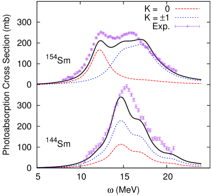
FIG. 1: (Color online) Photoabsorption cross sections of ${}^{144,154}$Sm from the FAM-QRPA calculation. The components from the $K=0$ and $K=\pm 1$ modes are also plotted. Here, $K=\pm 1$ refers to a sum of $+1$ and $-1$ modes. The experimental data is taken from Ref. 1974Carl.

Figure 1 shows a benchmark result of FAM-QRPA applied to the GDR. Here we plotted the photoabsorption cross sections obtained with the IVD strengths for ${}^{144,154}$Sm:

$$\sigma_{\rm abs}(\omega)=\frac{4\pi^{2}}{\hbar c}\omega\sum_{K=0,\pm 1}\frac{dB(\hat{\mathcal{D}}_{K};\omega)}{d\omega}.$$ (19)

The quadrupole matter distribution deformations of the HFB ground states are $\beta=0$ and $0.317$ for ${}^{144}$Sm and ${}^{154}$Sm, respectively. The IVD strengths of the $K=0$ and $\left|K\right|=1$ modes split in ${}^{154}$Sm due to the ground state deformation, whereas those are identical for spherical ${}^{144}$Sm. In both cases, FAM-QRPA shows a good agreement with the experimental data 1974Carl: the typical frequency and width of the GDR can be well reproduced with our model parameters, with the smearing width of $\Gamma=1.0$ MeV. The plateau distribution for the deformed ${}^{154}$Sm can be understood as a product of the split between $K=0$ and $\left|K\right|=1$ modes 2011Yoshida; 2013Yoshida. Our result also shows a good consistency to that of Ref. 2011Yoshida, in which MQRPA within the coordinate-space representation was adopted.

We have computed FAM strength function within the MPI parallelized scheme, where each part of the strength function was distributed on a separate core, similarly as in Ref. PhysRevC.92.051302. This scheme achieves a remarkable efficiency, enabling us to compute deformed heavier systems, where MQRPA is available only with a truncation of the model space. Typically, a computation of both of the $K$-modes took about 1500 CPU hours in a multicore Intel Sandy Bridge 2.6-GHz processor system.

TABLE 1: Ground state properties of Gd, Dy, and Er isotopes obtained with SkM* parameterization: axial deformation $\beta$, pairing gaps for neutrons and protons $(\Delta_{\rm n},\Delta_{\rm p})$, energy-weighted sum rule from Eq. (22), $m_{1}(\hat{\mathcal{D}}_{K})$, and its enhancement factor from the TRK sum rule $\kappa^{\rm IVD}$ (For SkM*, $\kappa^{\rm NM}=0.5315$).

Nuclide	$\beta$	$\Delta_{\rm n},~{}\Delta_{\rm p}$	$m_{1}(\hat{\mathcal{D}}_{K})$	$\kappa^{\rm IVD}$
		[MeV]	[$e^{2}$fm${}^{2}$MeV]
${}^{152}$Gd	$0.235$	$1.09,~{}1.19$	$253.9$	$0.3939$
${}^{154}$Gd	$0.301$	$1.16,~{}0.97$	$256.5$	$0.3944$
${}^{156}$Gd	$0.331$	$1.08,~{}0.89$	$258.9$	$0.3950$
${}^{158}$Gd	$0.346$	$1.05,~{}0.84$	$261.3$	$0.3953$
${}^{160}$Gd	$0.355$	$1.04,~{}0.80$	$263.6$	$0.3955$
${}^{162}$Gd	$0.358$	$1.07,~{}0.78$	$265.8$	$0.3955$
${}^{164}$Gd	$0.358$	$1.06,~{}0.76$	$267.9$	$0.3954$
${}^{156}$Dy	$0.289$	$1.17,~{}0.98$	$261.1$	$0.3944$
${}^{158}$Dy	$0.320$	$1.13,~{}0.88$	$263.7$	$0.3949$
${}^{160}$Dy	$0.336$	$1.10,~{}0.82$	$266.1$	$0.3954$
${}^{162}$Dy	$0.344$	$1.09,~{}0.78$	$268.5$	$0.3956$
${}^{164}$Dy	$0.347$	$1.09,~{}0.73$	$270.8$	$0.3957$
${}^{166}$Dy	$0.349$	$1.06,~{}0.69$	$273.0$	$0.3958$
${}^{168}$Dy	$0.348$	$1.01,~{}0.67$	$275.2$	$0.3959$
${}^{162}$Er	$0.324$	$1.15,~{}0.87$	$270.8$	$0.3953$
${}^{164}$Er	$0.334$	$1.14,~{}0.81$	$273.3$	$0.3957$
${}^{166}$Er	$0.339$	$1.12,~{}0.75$	$275.7$	$0.3959$
${}^{168}$Er	$0.342$	$1.08,~{}0.70$	$278.1$	$0.3962$
${}^{170}$Er	$0.342$	$1.00,~{}0.65$	$280.4$	$0.3964$
${}^{172}$Er	$0.337$	$0.97,~{}0.63$	$282.6$	$0.3965$
${}^{174}$Er	$0.329$	$1.06,~{}0.61$	$284.7$	$0.3964$

TABLE 2: The same as Table 1 but for Yb, Hf, and W isotopes.

Nuclide	$\beta$	$\Delta_{\rm n},~{}\Delta_{\rm p}$	$m_{1}(\hat{\mathcal{D}}_{K})$	$\kappa^{\rm IVD}$
		[MeV]	[$e^{2}$fm${}^{2}$MeV]
${}^{168}$Yb	$0.331$	$1.16,~{}0.60$	$280.5$	$0.3961$
${}^{170}$Yb	$0.335$	$1.10,~{}0.37$	$283.0$	$0.3966$
${}^{172}$Yb	$0.336$	$1.01,~{}0\phantom{0}\phantom{0}\phantom{0}$	$285.4$	$0.3970$
${}^{174}$Yb	$0.332$	$0.94,~{}0\phantom{0}\phantom{0}\phantom{0}$	$287.7$	$0.3973$
${}^{176}$Yb	$0.324$	$1.01,~{}0\phantom{0}\phantom{0}\phantom{0}$	$289.9$	$0.3972$
${}^{178}$Yb	$0.315$	$1.08,~{}0\phantom{0}\phantom{0}\phantom{0}$	$292.0$	$0.3970$
${}^{174}$Hf	$0.326$	$1.00,~{}0.85$	$290.1$	$0.3965$
${}^{176}$Hf	$0.316$	$0.97,~{}0.80$	$292.5$	$0.3970$
${}^{178}$Hf	$0.301$	$1.03,~{}0.74$	$294.8$	$0.3971$
${}^{180}$Hf	$0.288$	$1.06,~{}0.68$	$297.1$	$0.3970$
${}^{182}$Hf	$0.276$	$1.06,~{}0.64$	$299.2$	$0.3969$
${}^{184}$Hf	$0.263$	$1.03,~{}0.62$	$301.4$	$0.3969$
${}^{180}$W0	$0.270$	$1.09,~{}0.80$	$299.7$	$0.3971$
${}^{182}$W0	$0.257$	$1.11,~{}0.73$	$302.0$	$0.3972$
${}^{184}$W0	$0.245$	$1.10,~{}0.68$	$304.3$	$0.3972$
${}^{186}$W0	$0.230$	$1.07,~{}0.66$	$306.5$	$0.3973$
${}^{188}$W0	$0.212$	$1.01,~{}0.65$	$308.7$	$0.3974$
${}^{190}$W0	$0.191$	$0.97,~{}0.66$	$310.9$	$0.3974$

III.2 GDR in heavy rare-earth nuclei

Our survey of the GDR has been performed for even-even rare-earth nuclei from Gd ($Z=64$) to W ($Z=74$) isochains. Because several sets of experimental data are available 1981Gurevich; 1969Berman; 1976Gory, they can provide a more systematic check for FAM-QRPA GDR results. In Tables 1 and 2, we summarize the ground state properties of computed nuclei. The HFB calculation with SkM* concludes that all the nuclei considered here have rather stable prolate deformation.

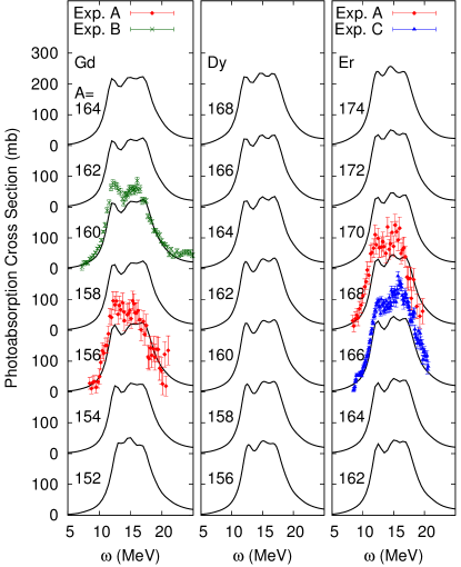
FIG. 2: (Color online) Photoabsorption cross sections of Gd, Dy, and Er isotopes as a function of photon energy. For FAM-QRPA calculation, the smearing width $\Gamma=1.0$ MeV is used. The experimental data sets A, B (photoabsorption), and C (neutron yield) are taken from Refs. 1981Gurevich, 1969Berman, and 1976Gory, respectively.

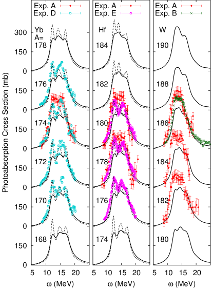
FIG. 3: (Color online) The same as Fig. 2 but for Yb, Hf, and W isotopes. The experimental data sets A, B(photoabsorption), D(neutron yield), and E(neutron product) are taken from Refs. 1981Gurevich, 1969Berman, 1976Gory2, and 1977Gory, respectively. For Yb and Hf, the results obtained with the smearing width of $\Gamma=0.5$ MeV are also plotted with dotted lines.

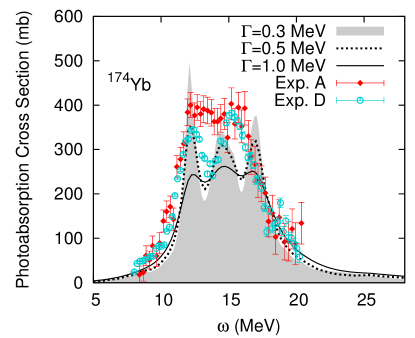
FIG. 4: (Color online) Photoabsorption cross sections of ${}^{174}$Yb obtained with different values of the smearing width $\Gamma$. The shown experimental data is the same as those in Fig. 3.

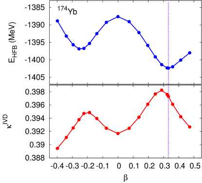
FIG. 5: (Color online) The total HFB energy and the IVD enhancement factor of ${}^{174}$Yb as a function of the axial deformation. The HFB ground state is indicated by the vertical dotted line.

Our results from FAM-QRPA are summarized in Figs. 2 and 3, in which the photoabsorption cross sections are compared with experimental data, where available. We emphasize here that experimental data in Refs. 1976Gory; 1976Gory2; 1977Gory does not correspond to total photoabsorption cross section, but the photo-neutron cross sections of $(\gamma,n)$ and $(\gamma,2n)$ type of reactions. Thus, it includes only a part of total photoabsorption cross section due to smaller number of output channels. Generally, we find a reasonable agreement between the FAM-QRPA and the experiments. Typical frequencies of GDR are fairly well reproduced throughout the rare-earth isotopes heavier than Sm. The width and the plateau top of the distribution are well understood as a product from the splitting of $K=0$ and $\left|K\right|=1$ modes, corresponding to the prolate deformation commonly found on their ground states. For ${}^{152}$Gd and several isotopes of W, the width of the GDR is graphically narrower than other nuclei, as expected due to smaller prolate deformation. In our HFB calculations, the proton pairing collapses for ${}^{172-178}$Yb. This collapse itself, however, does not make a significant impact on the GDR, as the GDR strength distributions look similar irrespective of the proton pairing collapse. Although the pairing could affect the GDR indirectly through the ground state properties (mainly deformation), their changes are small among the rare-earth nuclei, as shown in the present study.

There is an observed deficiency in the calculated photoabsorption cross sections at the region of heavier rare-earth isotopes, namely for $Z\geq 70$. For example, the calculated photoabsorption cross section of ${}^{174}$Yb underestimates the experimental data of Ref. 1981Gurevich at region $\omega=12-17$ MeV in which GDR becomes noticeably strong. A similar kind of GDR deficiency with Skyrme EDFs was reported in Ref. 2011Stetcu.

In Fig. 3, we have also plotted results for the Yb and Hf isotopes by using a smaller smearing width: $\Gamma=0.5$ MeV. With this smaller width, we can reproduce cross section of the neutron yield up to $\omega\approx 13$ MeV, which includes the first peak of the experimental data of Refs. 1976Gory2; 1977Gory. The second peak of the neutron yield cross section may be attributable to the opening of two-neutron emission channel: for ${}^{174}$Yb, for example, that peak locates at $\omega=15$ MeV, which is just above the two-neutron separation energy. With $\Gamma=0.5$ MeV, however, we could not achieve a complete improvement of aforementioned deficiency, and the total photoabsorption cross section remains underestimated. In Fig. 4, we also show that the narrower width of $\Gamma=0.3$ MeV leads computed photoabsorption cross sections to overshoot the experimental values at the peak positions, whereas a discrepancy at other frequencies remains. Consequently, the GDR deficiency found here is not improved by simply changing the smearing parameter $\Gamma$. Further systematic experiments of photoabsorption cross section, with improved accuracy, would be helpful by providing a more complete testing ground for theoretical models.

Theoretical deficiency of the GDR may be connected to the essential properties of the model. In order to remedy this deficiency, one could consider e.g. beyond QRPA effects or systematic adjustment of the EDF parameters. These are, however, beyond the scope of this article. Alternatively, we discuss a role of the TRK sum rule enhancement factor $\kappa^{\rm IVD}$, and its rule in the isovector dipole excitation 1995Rein; 1999Rein. This quantity can be related to the isovector effective mass of the infinite nuclear matter (INM), which can be used as an input parameter to define the Skyrme EDF parameters 2010Markus. Because there has been some ambiguity about the empirical value of this parameter, knowledge of its effect on GDR will be also profitable for the future optimization of the EDF parameters.

III.3 Energy-weighted sum rule

To discuss the sensitivity of GDR to the model parameters, we investigate the energy-weighted sum rule (EWSR), defined as

$$m_{1}(\hat{\mathcal{D}}_{K})=\int\omega\frac{dB(\hat{\mathcal{D}}_{K};\omega)}{d\omega}d\omega\,.$$ (20)

In terms of the transition matrix elements, it can be rewritten as

$$m_{1}(\hat{\mathcal{D}}_{K})=\sum_{i>0}\Omega_{i}\left|\Braket{i\mid\hat{\mathcal{D}}_{K}\mid 0}\right|^{2}\,.$$ (21)

It is well known that, by applying the Thouless theorem 1961Thouless, the EWSR based on the QRPA can be replaced with the expectation value of the double commutator of the HFB ground state 1973MdP; 2002Khan. For the present case this reads as

$$m_{1}(\hat{\mathcal{D}}_{K}) = \frac{1}{2}\Braket{0\mid[\hat{\mathcal{D}}_{K},~{}[\hat{H},\hat{\mathcal{D}}_{K}]~{}]\mid 0}$$ (22)

$$= (1+\kappa^{\rm IVD})\frac{e^{2}\hbar^{2}}{2m}\frac{NZ}{A}\frac{3}{4\pi},$$

where $\kappa^{\rm IVD}$ is the enhancement factor due to the momentum dependence of the effective interaction. For the Skyrme force, it can be given as

$$\kappa^{\rm IVD}=\frac{2m}{\hbar^{2}}(C^{\rho\tau}_{0}-C^{\rho\tau}_{1})\frac{A}{NZ}\int\rho_{\rm n}(\bm{r})\rho_{\rm p}(\bm{r})d\bm{r}.$$ (23)

For the IVD mode, the EWSR has the same value for $K=0$ and $1$ cases, even if the ground state is deformed. Note also that, for INM, $\kappa^{\rm NM}=2m(C^{\rho\tau}_{0}-C^{\rho\tau}_{1})\rho_{c}/\hbar^{2}$ is obtained.

Before going to applications, we check the validity of Eq. (22) in a generalized EDF framework 2015Hino. When the EDF is formally generalized, and has no correspondence with respect of the underlying effective force, Thouless theorem is not guaranteed to remain valid. Because we employed the Skyrme EDF combined with the mixed DDDP, the EWSR from actual QRPA calculations can deviate from Eq. (22). In Ref. 2015Hino, the authors showed that the Thouless theorem provides a reasonable approximation to the EWSR of the isoscalar/isovector monopole and quadrupole modes, even when Skyrme EDF lacks exact correspondence with respect to the underlying effective interaction but still holds the local gauge invariance. Here we give a similar test for the IVD mode.

For ${}^{174}$Yb, the energy-weighted sum rule, integrated from the transition strength function up to $\omega=50$ MeV, yields $m_{1}(\hat{\mathcal{D}}_{K})=283.9$ and $283.8$ $e^{2}$ fm${}^{2}$ MeV for $K=0$ and $K=1$ modes, respectively. Because of the deformation and the resultant splitting of $K=0$ and $K=1$ strengths, there is a small difference between two values. The contour integration technique of the complex-energy FAM, developed as an efficient tool to compute the sum rules in Ref. 2015Hino, yields $m_{1}(\hat{\mathcal{D}}_{K=0})=290.1$ $e^{2}$ fm${}^{2}$ MeV with an integration contour radius of $200$̃~{}MeV.Ontheotherside,thedoublecommutatorprocedureofEq.~{}(\ref{eq:EWSR3})gives$m_1($\hat{\mathcal{D}}$_K=0, ±1)=287.7 e^2$\,fm$^2$\,MeV,withenhancementfactorof$κ^IVD=0.397$,whenusingHFBprotonandneutrondensities.\par WefindthevaluefromthedoublecommutatormethodbeingconsistenttothosefromtheFAM-QRPAcalculation.Consequently,ThoulesstheoremcanprovideareliableapproximationoftheIVDsumrule.ThecomputationalcostforthedoublecommutatorprocedureisdrasticallylightercomparedtotheFAM-QRPA,sinceitrequiresinformationonlyabouttheHFBstate.\par\par WehavesummarizedtheEWSRvaluesandenhancementfactorsofEqs.~{}(\ref{eq:EWSR3})and(\ref{eq:EF_IVD})inTables\ref{tab:gs1}and\ref{tab:gs2}.ItisclearlyshownthattheenhancementfactorfortheTRKsumruleisalmostconstantatthisregionofthenuclearchart.Theratiooftwoenhancementfactors,\begin{equation}\frac{\kappa^{\rm IVD}}{\kappa^{\rm NM}}=\frac{A}{NZ\rho_{c}}\int\rho_{\rm n}(\bm{r})\rho_{\rm p}(\bm{r})d\bm{r}\,,\end{equation}isapproximately$0.74$forrare-earthsystemscalculatedherewithSkM*Skyrmeparameterization.ThisissimplyduetosimilarvalueobtainedfromthedensityintegrationofEq.~{}(\ref{eq:KR}),withonlyalimitedvariationontheprotonandneutrondensityprofileswithrespectof$N$and$Z$.\par InFig.~{}\ref{fig:beta_kappa},weplottheenhancementfactor$κ^IVD$andthetotalHFBenergy$E_HFB$asafunctionoftheaxialdeformationparameter$β$for$^174$Yb.TheseareobtainedfromtheHFBcalculationwithaconstrainton$β$.Approximately,theminimumofthetotalHFBenergycorrespondstothemaximumof$κ^IVD$.Thiscanbeunderstoodmainlyintermsofthesymmetryenergy,whichfavorsalargeoverlapbetweenneutronsandprotons.Duetootheringredients,especiallytheCoulombenergy,thetruegroundstateandmaximumof$κ^IVD$donotexactlycoincide.Thiscurveshows,however,thattheIVDenhancementfactorisnotverysensitivetothedetailsofthegroundstatedeformation.Next,weinvestigateifthedeficiencyagainsttheexperimentalphotoabsorptiondatafoundin$^174$Ybcouldbeimprovedbychanging$κ^NM$parameter.\text{TABLE 3Table 33TABLE 33TheINMTRKenhancementfactorκNMandm∗v/m,andthegroundstatepropertiesof}$