Vacuum energy density and pressure near a soft wall

Abstract

Perfectly conducting boundaries, and their Dirichlet counterparts for quantum scalar fields, predict nonintegrable energy densities. A more realistic model with a finite ultraviolet cutoff yields two inconsistent values for the force on a curved or edged boundary (the “pressure anomaly”). A still more realistic, but still easily calculable, model replaces the hard wall by a power-law potential; because it involves no a posteriori modification of the formulas calculated from the theory, this model should be anomaly-free. Here we first set up the formalism and notation for the quantization of a scalar field in the background of a planar soft wall, and we approximate the reduced Green function in perturbative and WKB limits (the latter being appropriate when either the mode frequency or the depth into the wall is sufficiently large). Then we display numerical calculations of energy density and pressure for the region outside the wall, which show that the pressure anomaly does not occur there. Calculations inside the wall are postponed to later papers, which must tackle regularization and renormalization of divergences induced by the potential in the bulk region.

I Introduction

The Casimir effect Milton ; BKMM ; Dalvit is traditionally thought of as a force between electrical conductors caused by the effects of these conducting boundaries on the spectrum of normal modes of the quantized electromagnetic field in the region exterior to the conductors. (For simplicity when investigating matters of principle, the EM field is often replaced by a scalar field, and the boundary conditions of a perfect conductor replaced by the Dirichlet condition, $\phi=0$. The present work deals with that model.) Crudely, the idea is that each mode acts as a harmonic oscillator with ground-state energy $\frac{1}{2}\omega$, so that when the energy is summed over all modes of the system, the total vacuum energy is $\langle E\rangle=\frac{1}{2}\sum_{n}\omega_{n}\,$; then the derivative of $\langle E\rangle$ with respect to some geometrical parameter of the system constitutes a generalized force, by the “principle of virtual work”.

This mode sum is clearly divergent, and its relation to physical realities measured in the laboratory has been somewhat controversial. Formal regularizations, such as the zeta-function method Elizalde , usually give answers that are generally accepted as “correct”, but their physical logic is unconvincing. Also, when the conductors are regarded as rigid and only their relative positions are allowed to vary, a finite answer for the force (or energy difference) can be obtained by sufficiently careful calculations BartonA ; Jaffe ; Schaden . It is generally agreed, however, that the root of the problem is the failure of the idealized notion of a perfect conductor. A real material does not act like a perfect conductor (or even a perfect dielectric) at very high frequencies, and thus nature must provide an ultraviolet (or high-momentum BartonB ) cutoff. But the detailed study of a real material is a complicated nonlinear problem of condensed-matter physics, and it is of interest to step back and see if the phenomena can still be modeled, at least qualitatively, entirely within the linear framework of the field alone.

The most common approach is to insert ad hoc an ultraviolet cutoff to make the integrals over frequency finite. The simplest choice is an exponential cutoff:

$$\langle E\rangle_{\tau}\equiv\frac{1}{2}\sum_{n}\omega_{n}e^{-\omega_{n}\tau},$$

where $\tau$ is the cutoff parameter, which can also be considered as a Wick rotation of the difference of two time coordinates, $\tau=-i(t-t^{\prime})$. A complementary approach is to calculate expectation values of the local energy density and pressure (components of the stress tensor: $u\equiv\langle T_{00}\rangle\,$, $p_{x}\equiv\langle T_{11}\rangle\,$, etc.), from which all the physically interesting quantities are in principle derivable. From local calculations one sees that, once one removes the ubiquitous zero-point energy that is present even for a completely free field, the vacuum energy density at any point away from the boundary is finite even without a cutoff, and infinities in the total energy (for a region of finite volume) arise only because the energy density is not integrable near the boundary. Thus this approach significantly elucidates the physical meaning of the divergences. Cutoff and local calculations fit very well together, as both can be based on a Green function of the field equation corresponding to the geometry of the system considered (e.g., rect ; HSW ).

It was reasonable to expect that keeping $\tau$ nonzero, and comparable (in natural units) to an interatomic spacing, would yield an effective model of the Casimir effects of a realistic imperfect conductor. However, when ultraviolet regularization is applied to the stress tensor, it produces formulas for energy density and pressure that are inconsistent with each other norman09 ; Estrada-Mera . The principle of virtual work, or energy-pressure balance, requires that a change in the vacuum energy corresponding to some infinitesimal movement of a boundary of the system be attributable to some vacuum pressure pushing against that boundary. As an example, consider the pressure against a flat wall,

$$-\,\frac{\partial E}{\partial x}=F=\iint p\,dy\,dz\qquad\left(E=\iiint u\,dx\,dy\,dz\right).$$ (1)

This relation does not follow by default from the local energy-momentum conservation law, ${\partial T^{\mu\nu}}/{\partial x^{\mu}}=0$ (which is satisfied by the expectation values inside the cavity). It instead constrains the equation of state of the quantized field (cf. TAnomaly ). It appears that the principle of virtual work has been disrupted by the regularization method. Pressure balance can be restored by replacing the timelike ultraviolet cutoff by point-splitting in a “neutral” direction, one parallel to the wall Estrada-Mera ; Benasque , but this is to repair the damage done by one ad hoc measure by adding another one.

Therefore, Bouas et al. SpecGeom proposed a new kind of model, the soft wall, wherein the Dirichlet boundary is replaced by a smooth, steeply rising potential function. Although regularization is still needed, as always in quantum field theory, the pathology of the perfect conductor has been removed in a physically rigorous way. That is, the departure from ideal conductivity is embodied from the start in a complete and consistent physical theory, rather than imposed a posteriori by inserting a cutoff into the formal mathematical results of an unrealistic theory. One has every reason to expect the principle of virtual work to hold (after renormalization) in this context.

Specifically, SpecGeom and HSW , summarized in Benasque , studied a “power wall” set at the plane $z=0$ (see Eq. (3)). It models a conducting plate whose thickness is much greater than its skin depth and whose size is large enough that edge effects are negligible. That project was continued in the thesis thesis , whose results are reported here with some corrections. Following Milton HSW , we express the components of the vacuum stress-energy tensor in terms of the reduced Green function formed from the solutions of the $z$ dependence of the field in the imaginary-frequency regime (Sec. II). In Sec. III we study those solutions analytically (in the limits of large and small frequency) and numerically. Energy density and pressure in the region outside the potential are plotted in Sec. IV; there, as expected, we find no indication of an anomaly in the energy-pressure balance. Sec. V sets up some machinery to be used in the future to tackle the more difficult problem of the interior of the wall, and Sec. VI summarizes the results and the outlook. Some references to older or tangentially related work that did not fit into this introduction are provided in an appendix.

II Formulation of the model

II.1 Field equation, basis solutions, and Green function

We consider the scalar field equation

$$\frac{\partial^{2}\Phi}{\partial t^{2}}=\nabla^{2}\Phi-V(z)\Phi,$$ (2)

where

$$V(z)=\begin{cases}0&\text{if }z\leq 0,\\ z^{\alpha}&\text{if }z>0,\end{cases}$$ (3)

is a scalar potential (or position-dependent Klein–Gordon mass). The field is classically real, hence Hermitian as a quantum field. The space-time coordinates are $(t,x,y,z)=(x^{0},x^{1},x^{2},x^{3})=\underline{x}$, and the metric tensor has signature $(-1,1,1,1)$. One often writes $r_{\perp}$ for $(x,y)$, and $k_{\perp}$ for the conjugate wave numbers, $(k_{1},k_{2})$. We use the natural units $\hbar=1=c$ and in addition choose the unit of length so that the coupling constant implied in Eq. (3) is unity; the fundamental length scale that emerges for a general coupling constant is identified in SpecGeom .

To avoid introducing gratuitous singular behavior around $z=0$, we take $\alpha$ to be a positive integer. As $\alpha\to\infty$, the potential formally approaches

$$V(z)=\begin{cases}0&\text{if }z<1,\\ \infty&\text{if }z>1,\end{cases}$$ (4)

which represents a hard wall (Dirichlet boundary condition) at $z=1$. Our goal is to understand the ground-state expectation values of energy density and pressure, which will be of significant magnitude only in some interval surrounding the interval $0\leq z\leq 1$.

When Eq. (2) is solved by separation of variables, the dimensions $(t,x,y)$ are trivial, and the $z$ dependence is given by solutions of

$$\bigg{(}-\frac{\partial^{2}}{\partial z^{2}}+V(z)-p^{2}\bigg{)}\phi(z)=0,$$ (5)

as detailed in SpecGeom . However, following HSW , we find it more useful to express vacuum expectation values in terms of a reduced Green function, built out of solutions of Eq, (5) with the sign of the spectral parameter reversed:

$$\bigg{(}-\frac{\partial^{2}}{\partial z^{2}}+V(z)+\kappa^{2}\bigg{)}\phi_{\kappa}(z)=0.$$ (6)

For each (positive) value of $p$ or $\kappa$, there are two linearly independent solutions of Eq. (5) or (6). Most obviously relevant are the solutions that decay as $z\to+\infty$; let $F(z)$ be such a solution, normalized at the origin for definiteness:

$$F(0)=1,\qquad\lim_{z\to\infty}F(z)=0.$$ (7)

A convenient choice of second solution is defined by

$$G(0)=0,\qquad G^{\prime}(0)=1.$$ (8)

In constructing the Green function, however, the most pertinent second solution is one that decays at $-\infty$:

$$H(0)=1,\qquad\lim_{z\to-\infty}H(z)=0.$$ (9)

It is sometimes convenient to relax the normalization conventions $F(0)=G^{\prime}(0)=H(0)=1$, and even the condition $G(0)=0$ (provided that $G$ and $F$ stay independent). When we give formulas that do not make those assumptions, we write the function names in the calligraphic font. For example, one notes immediately that for $z\leq 0$,

$$H_{\kappa}(z)=e^{\kappa z},$$ (10)

and hence that

$$\kappa=H_{\kappa}^{\prime}(0)=\frac{{\cal H}_{\kappa}^{\prime}(0)}{{\cal H}_{\kappa}(0)}\,.$$ (11)

For $z\geq 0$, the case $\alpha=1$ is easily solved using Airy functions, and the case $\alpha=2$ also produces an exact solution involving parabolic cylinder functions. For $\alpha=1$, the solutions (normalized as above) are

$$F_{\kappa}(z) =\frac{\operatorname{Ai}(\kappa^{2}+z)}{\operatorname{Ai}(\kappa^{2})}\,,$$ (12)

$$G_{\kappa}(z) =\frac{\operatorname{Bi}(\kappa^{2})\operatorname{Ai}(\kappa^{2}+z)-\operatorname{Ai}(\kappa^{2})\operatorname{Bi}(\kappa^{2}+z)}{\operatorname{Ai}^{\prime}(\kappa^{2})\operatorname{Bi}(\kappa^{2})-\operatorname{Ai}(\kappa^{2})\operatorname{Bi}^{\prime}(\kappa^{2})}\,.$$ (13)

For $\alpha=2$, the solutions are

$$F_{\kappa}(z) =\frac{\operatorname{D}_{-(\kappa^{2}+1)/2}(\sqrt{2}z)}{\operatorname{D}_{-(\kappa^{2}+1)/2}(0)}\,,$$ (14)

$$G_{\kappa}(z) =\frac{\operatorname{D}_{-(\kappa^{2}+1)/2}(-\sqrt{2}z)-\operatorname{D}_{-(\kappa^{2}+1)/2}(\sqrt{2}z)}{2\sqrt{2}\operatorname{D}_{(1-\kappa^{2})/2}(0)}\,.$$ (15)

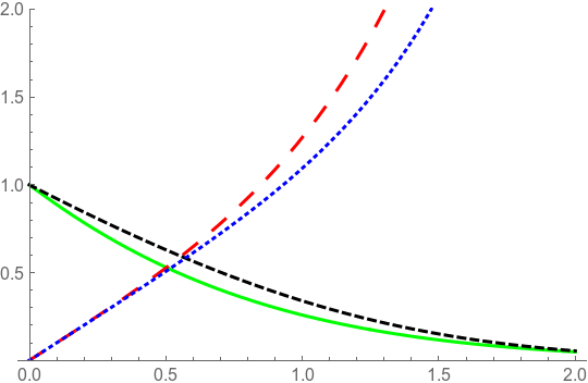
Figure 1: (color online) $F_{\kappa}(z)$ (solid, green) and $G_{\kappa}(z)$ (long dashed, red) for $\alpha=1$, $\kappa=1$, and $F_{\kappa}(z)$ (dashed, black) and $G_{\kappa}(z)$ (dotted, blue) for $\alpha=2$, $\kappa=0.5$, The differences between the two pairs of curves (in this region of small $z$) are caused more by the change in $\kappa$ than by the change in $\alpha$. All graphics in this paper were prepared with Mathematica.

In reference to the denominator in Eq. (15) see (NBS, , (19.6.2) and (19.3.5)). Examples of these functions are plotted in Fig. 1. Unfortunately, there are no known closed-form solutions to the differential equation when $\alpha>2$. Since we intend to examine the limiting case as $\alpha\to\infty$, we will need to find approximate solutions to these equations.

We denote the Wronskian of two solutions by

$$W(y_{1},y_{2})=y_{1}y_{2}^{\prime}-y_{1}^{\prime}y_{2}\,,$$ (16)

where the functions may be evaluated at any value of $z$, in particular at $z=0$.

The reduced Green function is to satisfy

$$\bigg{(}-\frac{\partial^{2}}{\partial z^{2}}+V(z)+\kappa^{2}\bigg{)}g_{\kappa}(z,z^{\prime})=\delta(z-z^{\prime}).$$ (17)

By a well known formula or method, one finds

$$g_{\kappa}(z,z^{\prime})=\frac{{\cal H}_{\kappa}(z_{<}){\cal F}_{\kappa}(z_{>})}{W({\cal F}_{\kappa},{\cal H}_{\kappa})}=\frac{{H}_{\kappa}(z_{<}){F}_{\kappa}(z_{>})}{\kappa-F^{\prime}_{\kappa}(0)}\,,$$ (18)

$$z_{<}=\min(z,z^{\prime}),\qquad z_{>}=\max(z,z^{\prime}).$$ (19)

Further reduction is postponed to later sections, because the most useful approach depends on whether one is working outside or inside the wall.

II.2 Stress tensor

The stress-energy-momentum tensor of a massless scalar field in flat space-time with curvature-coupling (conformal) parameter $\xi$ is

$$T_{\mu\nu}= \partial_{\mu}\Phi\partial_{\nu}\Phi-\frac{1}{2}g_{\mu\nu}(\partial_{\lambda}\Phi\partial^{\lambda}\Phi+V\Phi^{2})$$

$$-\xi(\partial_{\mu}\partial_{\nu}-g_{\mu\nu}\partial_{\lambda}\partial^{\lambda})\Phi^{2},$$ (20)

where $g_{\mu\nu}=\eta_{\mu\nu}=\text{diag}(-1,1,1,1)$. The equation of motion (2) can be used Gravity to rewrite Eq. (20) so that $V$ does not explicitly appear. Also, the notation

$$\beta=\xi-\tfrac{1}{4}$$ (21)

is convenient. Thus one arrives at these formulas for the energy density and pressure:

$$T_{00} =\frac{1}{2}(\partial_{0}\Phi)^{2}-\frac{1}{2}\Phi(\partial_{0})^{2}\Phi-\beta\nabla^{2}\Phi^{2},$$ (22a)

$$T_{11} =\frac{1}{2}(\partial_{1}\Phi)^{2}-\frac{1}{2}\Phi(\partial_{1})^{2}\Phi+\beta(-\partial_{0}^{2}+\partial_{2}^{2}+\partial_{3}^{2})\Phi^{2},$$ (22b)

and totally analogous expressions for $T_{22}$ and $T_{33}\,$. The remaining, off-diagonal, components of $T_{\mu\nu}$ play almost no role in our study; it is easy to show that their vacuum expectation values must vanish for a single, flat boundary as considered here (although they may temporarily develop nontrivial cutoff-dependent terms when point-splitting regularization is used with an oblique direction of point separation christensen ).

The expression of the vacuum expectation values $\langle T_{\mu\nu}\rangle$ in terms of Green functions has been detailed in previous papers SpecGeom ; HSW ; Benasque , but in a variety of formalisms. Here we shall not rehearse the standard quantum field theory leading to the main results, but rather concentrate on establishing consistent notations. On the one hand, the expectation value of the product of two field operators is a certain Green function for the wave equation,

$$\langle 0|\Phi(\underline{x})\Phi(\underline{x}^{\prime})|0\rangle=\frac{1}{i}G(\underline{x},\underline{x}^{\prime}),$$ (23)

of the form

$$G(\underline{x},\underline{x}^{\prime})=\int\frac{d\omega}{2\pi}\frac{d\text{\boldmath$k$}_{\perp}}{(2\pi)^{2}}e^{-i\omega(t-t^{\prime})}e^{i\text{\boldmath$k$}_{\perp}\cdot(\text{\boldmath$r$}_{\perp}-\text{\boldmath$r$}^{\prime}_{\perp})}g(p^{2};z,z^{\prime})$$ (24)

(all three integrations being over $(-\infty,\infty)$), with

$$p^{2}=\omega^{2}-\text{\boldmath$k$}_{\perp}^{2}$$ (25)

(which, despite the notation, is not necessarily positive). The vacuum energy density and pressure can now be found from Eq. (24) and the expectation values of Eqs. (22). If we set

$$\omega=i\zeta,\qquad t-t^{\prime}=i(\tau-\tau^{\prime}),$$ (26)

and formally rotate the $\zeta$ integration back to the real axis, we get

$$-iG(\underline{x},\underline{x}^{\prime})=\int\frac{d\zeta}{2\pi}\frac{d\text{\boldmath$k$}_{\perp}}{(2\pi)^{2}}e^{i(\zeta\tau+\text{\boldmath$k$}_{\perp}\cdot\text{\boldmath$r$}_{\perp})}g_{\kappa}(z,z^{\prime}),$$ (27)

which we have here simplified by setting $\tau^{\prime}$ and $\text{\boldmath$r$}^{\prime}_{\perp}$ equal to zero. We now have

$$\kappa^{2}=\zeta^{2}+\text{\boldmath$k$}_{\perp}^{2},$$ (28)

which is always positive. On the other hand, the calculation of the expectation values can be based from the outset on the “cylinder kernel”, a certain Green function for the equation

$$\frac{\partial^{2}\Phi}{\partial\tau^{2}}+\nabla^{2}\Phi-V(z)\Phi=0.$$ (29)

Standard construction of that function leads rigorously to Eq. (27), times $-2$:

$$\overline{T}(\tau,\text{\boldmath$r$}^{\prime}_{\perp},z,z^{\prime})=-2\int\frac{d\zeta}{2\pi}\frac{d\text{\boldmath$k$}_{\perp}}{(2\pi)^{2}}e^{i(\zeta\tau+\text{\boldmath$k$}_{\perp}\cdot\text{\boldmath$r$}_{\perp})}g_{\kappa}(z,z^{\prime}),$$ (30)

with $\kappa$ defined as the positive root of Eq. (28).

The next step of the calculation is most simply expressed by writing the vacuum stress as a Fourier transform:

$$\langle T_{\mu\nu}\rangle=\int\frac{d\zeta}{2\pi}\frac{d\text{\boldmath$k$}_{\perp}}{(2\pi)^{2}}e^{i\zeta\tau}e^{i\text{\boldmath$k$}_{\perp}\cdot\text{\boldmath$r$}_{\perp}}t_{\mu\nu}\Big{|}_{z^{\prime}\rightarrow z}.$$ (31)

From Eqs. (22), (23), and (27) one gets

$$t_{00} =-\zeta^{2}g_{\kappa}(z,z)-2\beta(\partial_{z}^{2}+\partial_{z}\partial_{z}^{\prime})g_{\kappa}(z,z^{\prime})\big{|}_{z^{\prime}\rightarrow z},$$ (32a)

$$t_{11} =k_{1}^{2}g_{\kappa}(z,z)+2\beta(\partial_{z}^{2}+\partial_{z}\partial_{z}^{\prime})g_{\kappa}(z,z^{\prime})\big{|}_{z^{\prime}\rightarrow z},$$ (32b)

$$t_{22} =k_{2}^{2}g_{\kappa}(z,z)+2\beta(\partial_{z}^{2}+\partial_{z}\partial_{z}^{\prime})g_{\kappa}(z,z^{\prime})\big{|}_{z^{\prime}\rightarrow z},$$ (32c)

$$t_{33} =-\,\frac{1}{2}(\partial_{z}^{2}-\partial_{z}\partial_{z}^{\prime})g_{\kappa}(z,z^{\prime})\big{|}_{z^{\prime}\rightarrow z}.$$ (32d)

It is noteworthy that $\langle T_{33}\rangle$ is independent of $\beta$ (or $\xi$).

Note that primed coordinates other than $z^{\prime}$, and derivatives with respect to them, have been eliminated, so without loss of generality we may set those coordinates equal to $0$. Now the 4-vector

$$\text{\boldmath$\delta$}=(\tau,\text{\boldmath$r$}_{\perp},(z-z^{\prime}))$$ (33)

should be regarded as the separation between the two space-time points that are arguments of the fields in the quadratic field observables; it is still needed to regularize the formulas for the vacuum energy and pressure. In the present work, however, we have no need to consider splitting in the $z$ direction, so we can set $z^{\prime}=z$ as soon as the derivatives indicated in Eqs. (32) have been taken. To understand the pressure anomaly it is essential, though, to consider point-splitting in an arbitrary direction in the $(\tau,\text{\boldmath$r$}_{\perp})$ 3-space Estrada-Mera ; sector1 .

Putting Eqs. (31) and (32) together, we obtain formulas for $\langle T_{\mu\nu}\rangle$. For example, the energy formula is

$$\langle T_{00}\rangle= \int\frac{d\zeta}{2\pi}\frac{d\text{\boldmath$k$}_{\perp}}{(2\pi)^{2}}e^{i\zeta\tau+i\text{\boldmath$k$}_{\perp}\cdot\text{\boldmath$r$}_{\perp}}$$ (34)

$$\times[-\zeta^{2}g_{\kappa}(z,z)-2\beta(\partial_{z}^{2}+\partial_{z}\partial_{z}^{\prime})g_{\kappa}(z,z^{\prime})\big{|}_{z^{\prime}\rightarrow z}].$$

After $z^{\prime}$ is taken to $z$, the $\delta$ of Eq. (33) can be thought of as a 3-vector and the exponent in Eq. 34 can be written $\text{\boldmath$\kappa$}\cdot\text{\boldmath$\delta$}$, where

$$\text{\boldmath$\kappa$}=(\zeta,\text{\boldmath$k$}_{\perp}).$$ (35)

As in HSW , we make a change of variables to polar coordinates, defined by

$$\kappa^{2} =\lvert\text{\boldmath$k$}_{\perp}\rvert^{2}+\zeta^{2}, \quad\cos{\theta} =\frac{\zeta}{\kappa}\,,$$ (36a)

$$\delta^{2} =\lvert\text{\boldmath$r$}_{\perp}\rvert^{2}+\tau^{2}, \quad\cos{\phi} =\frac{k_{1}}{\lvert\text{\boldmath$k$}_{\perp}\rvert}\,.$$ (36b)

Note next that $z^{\prime}$ can be completely eliminated from Eqs. (32a)–(32c) by recognizing the total derivative

$$\frac{d^{2}}{dz^{2}} \Big{[}g_{\kappa}(z,z^{\prime})\big{|}_{z^{\prime}\rightarrow z}\Big{]}$$

$$=2\Big{[}\frac{\partial^{2}}{\partial z^{2}}g_{\kappa}(z,z^{\prime})\big{|}_{z^{\prime}\rightarrow z}+\frac{\partial}{\partial z}\frac{\partial}{\partial z^{\prime}}g_{\kappa}(z,z^{\prime})\big{|}_{z^{\prime}\rightarrow z}\Big{]}.$$ (37)

We then rewrite Eq. (34) as

$$\langle T_{00}\rangle= \frac{1}{(2\pi)^{3}}\Bigg{(}\frac{\partial^{2}}{\partial\tau^{2}}-\beta\frac{\partial^{2}}{\partial z^{2}}\Bigg{)}\int_{0}^{\infty}d\kappa\,\kappa^{2}\int_{-1}^{1}d\cos{\theta}$$

$$\times\int_{0}^{2\pi}d\phi\,e^{i\kappa\sin{\theta}(\cos{\phi}\,r_{1}+\sin{\phi}\,r_{2})}e^{i\kappa\cos{\theta}\,\tau}g_{\kappa}(z,z)$$ (38)

and integrate over the angular coordinates. Doing the same for the other components, we finally arrive at the expectation values of the stress-energy tensor components:

$$u\equiv\langle T_{00}\rangle =\frac{1}{2\pi^{2}}\bigg{(}\frac{\partial^{2}}{\partial\tau^{2}}-\beta\frac{\partial^{2}}{\partial z^{2}}\bigg{)}\int_{0}^{\infty}d\kappa\,\kappa g_{\kappa}(z,z)\frac{\sin{\kappa\delta}}{\delta}\,,$$ (39a)

$$p_{x}\equiv\langle T_{11}\rangle =\frac{1}{2\pi^{2}}\bigg{(}-\frac{\partial^{2}}{\partial r_{1}^{2}}+\beta\frac{\partial^{2}}{\partial z^{2}}\bigg{)}\int_{0}^{\infty}d\kappa\,\kappa g_{\kappa}(z,z)\frac{\sin{\kappa\delta}}{\delta}\,,$$ (39b)

$$p_{y}\equiv\langle T_{22}\rangle =\frac{1}{2\pi^{2}}\bigg{(}-\frac{\partial^{2}}{\partial r_{2}^{2}}+\beta\frac{\partial^{2}}{\partial z^{2}}\bigg{)}\int_{0}^{\infty}d\kappa\,\kappa g_{\kappa}(z,z)\frac{\sin{\kappa\delta}}{\delta}\,,$$ (39c)

$$p_{z}\equiv\langle T_{33}\rangle =-\,\frac{1}{4\pi^{2}}\int_{0}^{\infty}d\kappa\,\kappa\bigg{[}\bigg{(}\frac{\partial^{2}}{\partial z^{2}}-\frac{\partial}{\partial z}\frac{\partial}{\partial z^{\prime}}\bigg{)}g_{\kappa}(z,z^{\prime})\bigg{]}\bigg{|}_{z^{\prime}\rightarrow z}$$

$$\quad\times\frac{\sin{\kappa\delta}}{\delta}\,.$$ (39d)

It is readily seen that the only dependence remaining on the point-splitting vector inside the integral is in the scalar $\delta$, which depends on the differentiation variables $(\tau,\text{\boldmath$r$}_{\perp})$ in a symmetrical way. If there were no divergences, we would now find the physical energy density and pressure by taking $\delta\rightarrow 0$. In that limit, formally $u=-p_{x}=-p_{y}\,$, which is the expected relation between energy density and pressure as predicted by the principle of virtual work. To visualize this fact, place a test wall (say the $x$–$z$ plane) perpendicular to the existing soft wall. If a pressure $p_{x}$ pushes the test wall, there should be a decrease in energy corresponding to the amount of work done in the process of moving the test wall; since $u$ is independent of the position of the test wall, this energy change is simply $u$ times the displacement. Thus Eq. (1) is satisfied — in fact, the integrands on the two sides are pointwise the same. Thus, insofar as the integrals in Eqs. (39) converge, no pressure anomaly arises. We must now examine the precise situation outside and inside the wall separately (Secs. IV and V).

III Perturbation theory

When either $z$ or $\kappa$ is large, solutions of Eq. (6) in the potential region are well approximated by the (Carlini–Liouville–Green–Jeffreys–) WKB method for the exponential (nonoscillatory) regime. Since the theory and formulas are well known, we shall simply introduce the expressions when needed.

When both $z$ and $\kappa$ are small, a different approximation method is needed. One can write a solution of Eq. (6) as a power series in $\kappa^{2}$. To first order,

$$F_{\kappa}(z) \approx F_{0}(z)+\kappa^{2}F_{1}(z),$$ (40a)

$$G_{\kappa}(z) \approx G_{0}(z)+\kappa^{2}G_{1}(z).$$ (40b)

Luckily, the equation can be solved exactly when $\kappa=0$. We introduce the notations

$$b=\frac{1}{\alpha+2}\,,$$ (41)

$$k(z) =\sqrt{z}K_{b}\!\left(2bz^{\frac{1}{2b}}\right)\,,$$ (42a)

$$i(z) =\sqrt{z}I_{b}\!\left(2bz^{\frac{1}{2b}}\right)\,,$$ (42b)

where $K$ and $I$ are the modified Bessel functions. Then

$$F_{0}(z) =c_{1}\,k(z),$$ (43a)

$$G_{0}(z) =c_{2}\,i(z),$$ (43b)

where $c_{1}$ and $c_{2}$ are constants used to match the normalization conditions (7) and (8).

$F_{1}$ must be of the form

$$F_{1}(z)=\int_{0}^{\infty}g(z,z^{\prime})F_{0}(z^{\prime})\,dz^{\prime},$$ (44)

$g$ being a suitable Green function for the nonhomogeneous equation

$$F_{1}^{\prime\prime}-z^{\alpha}F_{1}=F_{0}\,.$$ (45)

By hypothesis $c_{1}$ has already been chosen to match the boundary data exactly, so the proper solution must satisfy $F_{1}(0)=0$ as well as vanishing at infinity. Therefore,

$$g(z,z^{\prime})=\frac{i(z_{<})k(z_{>})}{W(i,k)}\,.$$ (46)

The solution for $G_{1}$ is similar, but this time the Green function must annihilate both $G(0)$ and $G^{\prime}(0)$, with no condition at infinity. Thus we arrive at

$$F_{1}(z) =\frac{1}{W(i,k)}\left(k(z)\int_{0}^{z}i(a)F_{0}(a)\,da+i(z)\int_{z}^{\infty}k(a)F_{0}(a)\,da\right),$$ (47a)

$$G_{1}(z) =\frac{1}{W(i,k)}\left(k(z)\int_{0}^{z}i(a)G_{0}(a)\,da-i(z)\int_{0}^{z}k(a)G_{0}(a)\,da\right),$$ (47b)

where the Wronskian is defined as in Eq. (16).

In Figures 2–5 the exact Airy-function solutions with $\alpha=1$ are compared with the perturbative and the WKB approximations, for various values of $\kappa$. As expected, as $\kappa$ grows there is a transition from perturbative to WKB regime. The WKB formulas used here are the first-order ones,

$$F(z) \approx c_{F}(\kappa^{2}+z^{\alpha})^{-\frac{1}{4}}\exp\left[-\int dz\left(\sqrt{\kappa^{2}+z^{\alpha}}\right)\right],$$ (48a)

$$G(z) \approx c_{G}(\kappa^{2}+z^{\alpha})^{-\frac{1}{4}}\sinh\left[\int dz\left(\sqrt{\kappa^{2}+z^{\alpha}}\right)\right].$$ (48b)

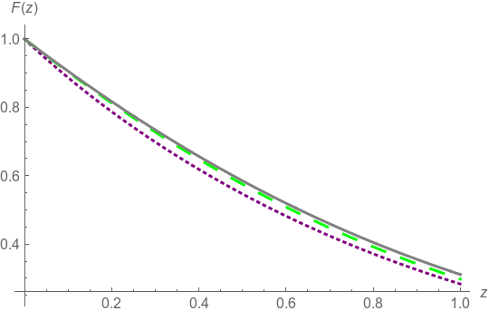
Figure 2: (color online) Exact (solid, gray), perturbation (long dashed, green), and WKB (dotted, purple) solutions of $F(z)$ for $\alpha=1$, $\kappa=0.7$. The perturbation solution closely matches the exact solution.

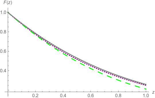
Figure 3: (color online) Exact (solid, gray), perturbation (long dashed, green), and WKB (dotted, purple) solutions of $F(z)$ for $\alpha=1$, $\kappa=1$. The WKB solution closely matches the exact solution.

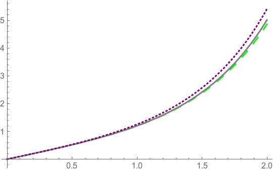
Figure 4: (color online) Exact (solid, gray), perturbation (long dashed, green), and WKB (dotted, purple) solutions of $G(z)$ for $\alpha=1$, $\kappa=0.8$. The perturbation solution closely matches the exact solution.

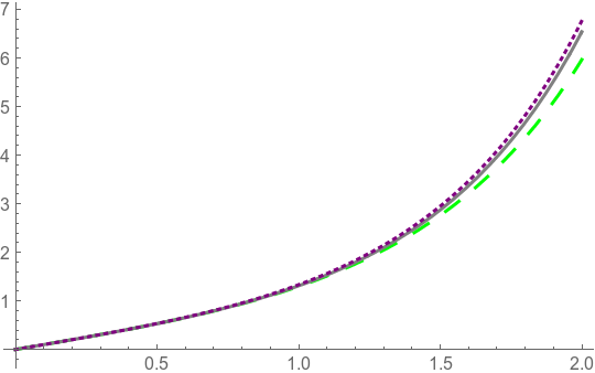
Figure 5: (color online) Exact (solid, gray), perturbation (long dashed, green), and WKB (dotted, purple) solutions of $G(z)$ for $\alpha=1$, $\kappa=1.1$ The WKB solution closely matches the exact solution.

Calculations with special functions determine that

$$W(i,k)=-\,\frac{3}{2}\,,\quad c_{1}=\frac{2b^{b}}{\Gamma(b)}\,,\quad c_{2}=\frac{\Gamma(b)}{3b^{b}}\,.$$ (49)

and hence that

$$F_{0}^{\prime}(0)=-b^{2b-1}\frac{\Gamma(1-b)}{\Gamma(b)}\,,\qquad F_{1}^{\prime}(0)=-\,\frac{\sqrt{\pi}b^{1-2b}}{2^{4b-1}}\,\frac{\Gamma(2b)\Gamma(3b)}{\Gamma(b)\Gamma\left(\frac{1}{2}+2b\right)}\,.$$ (50)

We remark that higher-order $z$-derivatives at $0$ may not exist, because fractional powers of $z$ arise in the expansion of $k(z)$.

The perturbative expansion of $F_{\kappa}$ may be applied with negative values of $\kappa^{2}$ to approximate the eigenfunctions, solutions of Eq. (5).

Conceptually it is easy to extend the perturbative expansions to higher order in $\kappa^{2}$ by formulas of the structure

$$F_{n}(z)=\int dz_{1}\cdots dz_{n}\,g(z,z_{1})\cdots g(z_{n-1},z_{n})F_{0}(z_{n}).$$ (51)

We have not implemented any order above the first, because the iterated numerical integrations would become demanding. We tried a second-order WKB approximation but found, as usual for a nonconvergent asymptotic series, that it made the results worse in the region of moderate $z$ where an improvement was most needed.

IV Outside the wall

When $z\leq 0$, ${\cal F}_{\kappa}(z)$ has the form $c_{-}(\kappa)(e^{-\kappa z}+\gamma_{-}(\kappa)e^{\kappa z})$. A calculation from the boundary data (7) yields

$$\gamma_{-}(\kappa)=\frac{\kappa{\cal F}_{\kappa}(0)+{\cal F}^{\prime}_{\kappa}(0)}{\kappa{\cal F}_{\kappa}(0)-{\cal F}^{\prime}_{\kappa}(0)}=\frac{\kappa+{F}^{\prime}_{\kappa}(0)}{\kappa-{F}^{\prime}_{\kappa}(0)}\,.$$ (52)

Thus, when both $z$ arguments are negative, the Green function (18) reduces to HSW

$$g_{\kappa}(z,z^{\prime})=\frac{1}{2\kappa}e^{-\kappa|z-z^{\prime}|}+\frac{1}{2\kappa}e^{\kappa(z+z^{\prime})}\gamma_{-}(\kappa).$$ (53)

The first term in Eq. (53) is the Green function for empty Minkowski space, which is the same regardless of the presence of the wall. This term has been exhaustively studied already; more can be read about it in almost any introductory text on the Casimir effect (for example, CasReview ) and, with special reference to point-splitting regularization, in christensen . Christensen’s formula (christensen, , Eq. (6.2)) does exhibit a dependence on the direction of point-splitting in a way that differs from one component of $\langle T_{\mu\nu}\rangle$ to the next and hence would be considered “anomalous” in the sense of Estrada-Mera if the point separation were to be regarded as a physical regularization to be kept nonzero at the end. That is, however, never done; the direction-dependent terms are argued away as artifacts of a noncovariant regularization procedure, and the entire Minkowski-vacuum stress tensor is set equal to either zero or a multiple of $g_{\mu\nu}$ (cosmological constant term) zeldovich ; christensen2 ; ALN2 ; Benasque .

Returning to the second term in Eq. (53), one sees that it contains all of the effects of the wall on space outside the wall (i.e., for $z<0$). Furthermore, because of the rapid decrease of that term as $\kappa\to\infty$, its contributions to the energy density and pressure are continuous and convergent as $\text{\boldmath$\delta$}\to 0$. So, we may now set $\delta=0$ and $z^{\prime}=z$, and as pointed out in Sec. II.2 we may be confident that the two pressures parallel to the wall are equal to $-u$. The perpendicular pressure $p_{z}$ now also works out correctly: In the limit $\delta\rightarrow 0$, the integrand of Eq. (39d) becomes identically zero for all values of $\kappa$, so $p_{z}=0$. This confirms the principle of virtual work, because the total energy of the system does not change when the soft wall moves perpendicularly to itself: the boundary energy density is concentrated near the boundary and is merely dragged along with the wall. (However, the pressure acting on the boundary from the right from inside the wall remains to be investigated.) Finally, as in HSW , Eq. (39a) reduces to

$$u(z)=\frac{1-6\xi}{6\pi^{2}}\int_{0}^{\infty}d\kappa\kappa^{3}e^{2\kappa z}\gamma_{-}(\kappa).$$ (54)

(We emphasize that the Minkowski zero-point energy has already been removed from this quantity, which was called $u(z)-u_{0}$ in HSW .)

The next task is to find a good approximation to $\gamma_{-}(\kappa)$. At small $\kappa$ we can use the perturbative formulas (40) and (50) to get and evaluate

$$\gamma_{-}(\kappa)\approx\frac{\kappa+F^{\prime}_{0}(0)+\kappa^{2}F^{\prime}_{1}(0)}{\kappa-F^{\prime}_{0}(0)-\kappa^{2}F^{\prime}_{1}(0)}.$$ (55)

At large $\kappa$, using a WKB formula one finds an accidental cancellation in (52) such that it predicts $\gamma_{-}$ identically zero. To get a nontrivial result, we perform the reweighting of terms carried out in (HSW, , Sec. IV) to arrive at (HSW, , Eq. (4.29))

$$\gamma_{-}(\kappa)\approx-\,\frac{\Gamma(\alpha+1)}{(2\kappa)^{\alpha+2}}.$$ (56)

(It is clear that this leading term would appear in a WKB calculation only at a rather high order, increasing with $\alpha$.)

For $\alpha=1$ and $2$ these two approximations can be tested against exact calculations from Eqs. (12) and (14). They match $\gamma_{-}(\kappa)$ very well for small and large $\kappa$, respectively, but there is a significant intermediate region in which neither is accurate. After some experimentation, we remedied this very well by introducing the spline function

$$s(\kappa)=e^{a+b\kappa},$$ (57)

where $a$ and $b$ are chosen so that the functions match at the endpoints of a central interval $[d_{1},d_{2}]$,

$$s(d_{1}) =\frac{F^{\prime}_{0}(0)+d_{1}+d_{1}^{2}F^{\prime}_{1}(0)}{F^{\prime}_{0}(0)-d_{1}+d_{1}^{2}F^{\prime}_{1}(0)}$$ (58)

$$s(d_{2}) =\frac{\Gamma(\alpha+1)}{(2d_{2})^{\alpha+2}}\,,$$ (59)

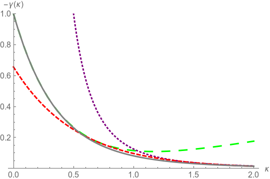
Figure 6: (color online) Approximations (perturbation in long green dashes, Milton (56) in purple dots, spline in red dashes) and exact solution (solid gray) for $-\gamma_{-}$ in the case $\alpha=1$.

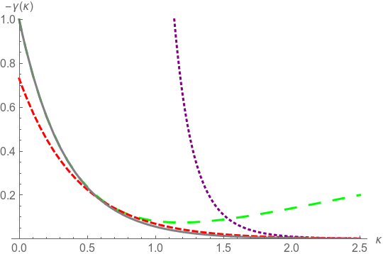
Figure 7: (color online) Approximations (perturbation in long green dashes, Milton in purple dots, spline in red dashes) for $-\gamma_{-}$ in the case $\alpha=6$. A numerical approximation of the exact solution is shown in solid gray. Notice that the spline matches the exact function well even when the two asymptotic approximations are far apart.

and then $d_{1}$ and $d_{2}$ are chosen so that the derivatives also match there (by an application of Newton’s method in Mathematica). (The exponential spline is superior to a linear one because it qualitatively reproduces the obvious convex behavior of $\gamma_{-}(\kappa)$.) We approximate $|\gamma_{-}(\kappa)|$ by a piecewise-defined function given by the perturbation solution when $\kappa<d_{1}\,$, the spline function (57) when $d_{1}<\kappa<d_{2}\,$, and the large-$\kappa$ solution when $d_{2}<\kappa$. Since this piecewise function is seen to be strictly greater than the exact solution, our value for $u(z)$ will be an upper bound. Some plots of these approximations are given in Figs. 6 and 7, with comparisons to the exact Airy formula for $\alpha=1$ and to a numerical solution for $\alpha=6$.

Now that we have $\gamma_{-}(\kappa)$, we can find the energy density outside the wall by numerical integration of Eq. (54). Representative resulting plots are in Figs.  8 and 9. As anticipated in HSW , the integral for $u(0)$ converges only for $\alpha>2$. The present method is a significant improvement over the preliminary treatment in HSW in regards to the contributions from small $\kappa$.

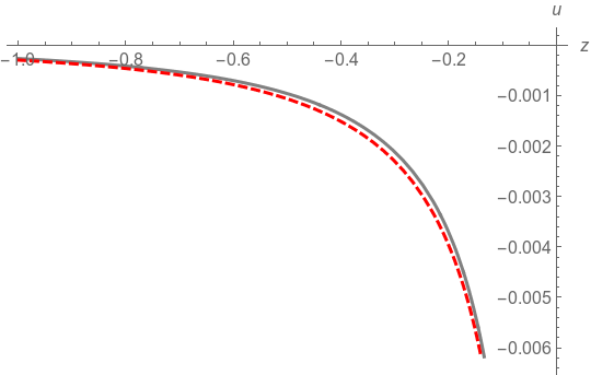
Figure 8: (color online) Approximation (dashed) and exact solution (solid) for $\langle T_{00}\rangle$ outside the wall in the $\alpha=1$ case. The factor $1-6\xi$ is omitted. The vertical axis is an asymptote.

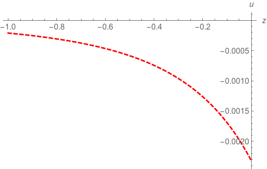
Figure 9: (color online) Approximation for $\langle T_{00}\rangle$ outside the wall in the $\alpha=6$ case. The factor $1-6\xi$ is omitted. The vertical axis has an intercept.

V Inside the wall

The problem of finding the energy density inside the wall, where the potential is nonzero, is substantially more difficult than the case outside the wall. First, we need to compute not only the coefficient $\gamma_{+}(\kappa)$ but also the solutions $F_{\kappa}(z)$ and $G_{\kappa}(z)$, functions of two variables. Second, there are divergences “in the bulk” proportional to local functionals of the potential, which need to be identified and removed by renormalization in the usual sense of quantum field theory MNS . Third, the Green function does not divide neatly and uniquely into two terms, one purely divergent and the other containing all the real physics, as happened in Eq. (53). Finally, at small $\kappa$ it is difficult to normalize WKB solutions properly, since the boundary conditions (7) and (8) must be applied at $0$, precisely where the WKB approximation is least valid. It is this last nuisance that forces us to consider the whole family of more general normalization conventions.

We begin, as we did in the previous section, by expressing the Green function more explicitly in terms of the basis functions. Let

$$H_{\kappa}=c_{+}(\kappa)({\cal G}_{\kappa}+\gamma_{+}(\kappa){\cal F}_{\kappa})$$ (60)

(thereby defining $c_{+}$ and $\gamma_{+}$). Then

$$\gamma_{+}(\kappa)=-\,\frac{\kappa{\cal G}_{\kappa}(0)-{\cal G}_{\kappa}^{\prime}(0)}{\kappa{\cal F}_{\kappa}(0)-{\cal F}^{\prime}_{\kappa}(0)}=\frac{1}{\kappa-F^{\prime}_{\kappa}(0)}\,.$$ (61)

It follows that

$$g_{\kappa}(z,z^{\prime})=c_{+}(\kappa)\frac{\left({\cal G}_{\kappa}(z_{<})+\gamma_{+}(\kappa){\cal F}_{\kappa}(z_{<})\right){\cal F}_{\kappa}(z_{>})}{W({\cal F}_{\kappa},e^{\kappa z})}=\left(G_{\kappa}(z_{<})+\gamma_{+}(\kappa)F_{\kappa}(z_{<})\right)F_{\kappa}(z_{>}).$$ (62)

Because $W({\cal F},e^{\kappa z})=c_{+}W({\cal F},{\cal G})$, the middle (generic) version of Eq. (62) reduces to

$$g_{\kappa}(z,z^{\prime})=\frac{{\cal G}_{\kappa}(z_{<}){\cal F}_{\kappa}(z_{>})}{W({\cal F}_{\kappa},{\cal G}_{\kappa})}+\gamma_{+}(\kappa)\frac{{\cal F}_{\kappa}(z){\cal F}_{\kappa}(z^{\prime})}{W({\cal F}_{\kappa},{\cal G}_{\kappa})},$$ (63)

which is (HSW, , Eq. (4.5)). Here the generic formula for $\gamma_{+}$ (the middle member of Eq. (61)) must be used.

Because of the freedom to redefine $\cal G$ by adding a multiple of $\cal F$, the division of $g_{\kappa}$ in Eq. (63) into two terms is rather arbitrary. In the extreme case that ${\cal G}={\cal H}$, the second term vanishes completely. Ideally one would like to go to the opposite extreme and make the first term “purely divergent”, so that all the interesting physics is in the second term. (Note that, because of rapid decay as function of $\kappa$, the second term yields convergent integrals that are continuous functions of the point separation $\delta$, so one can set the points equal before trying to evaluate them.) The convention ${\cal G}_{\kappa}(0)=0$ is certainly not that ideal; it makes the first term in $g_{\kappa}$ into the Green function for a problem with a Dirichlet condition at $z=0$, and the resulting vacuum stress will have the singular behavior associated with a perfectly reflecting boundary there. Since our real problem does not have such a boundary, but only a mild coefficient singularity that weakens with increasing $\alpha$ (see (WKBwall, , p. 25) and (SpecGeom, , p. 146)), these boundary terms must be cancelled by contributions from the second term.

We present here a preliminary numerical exploration in the spirit of the previous section, starting with lowest-order approximations for $\gamma_{+}(\kappa)$. One can use the WKB form of $F(z)$ in the high $\kappa$ region to find the leading term

$$\gamma_{+}(\kappa)\approx\frac{1}{2\kappa}\,.$$ (64)

In the region of small $\kappa$, one approximates $F_{\kappa}^{\prime}(0)\approx F_{0}^{\prime}(0)$ to get

$$\gamma_{+}(\kappa)\approx\frac{1}{\kappa+b^{2b-1}\Gamma(1-b)/\Gamma(b)}$$ (65)

where $b=(\alpha+2)^{-1}$ as before.

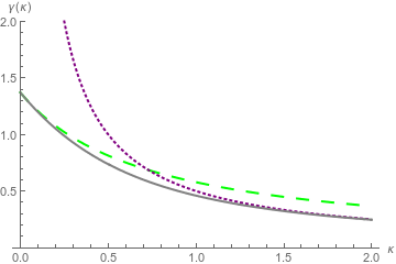
Figure 10: (color online) $\gamma^{+}(\kappa)$ for $\alpha=1$. The solid gray line is the exact solution, the long-dashed green line is the perturbation expansion, and the dotted purple line is the WKB approximation.

Although the results in Fig. 10 are as expected, we then found that the spline technique we used for $\gamma_{-}$ does not work as well for $\gamma_{+}\,$; details would be premature here.

We proceed to tackle the Green function. In creating Figs. 11–12 we used the perturbative form of $\gamma_{+}(\kappa)$ and the perturbative solutions (40), (47) for $F_{\kappa}(z)$ and $G_{\kappa}(z)$ to obtain a “perturbative approximation”, and the WKB form of $\gamma_{+}(\kappa)$ and the WKB solutions (48) for $F_{\kappa}(z)$ and $G_{\kappa}(z)$ to obtain a “WKB approximation”. As expected, Fig. 11 shows that the perturbative expansion is good for a small $\kappa$, and Fig. 12 shows that the WKB expansion is good for a large $\kappa$.

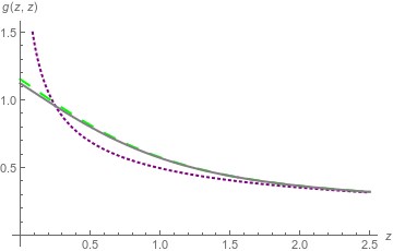
Figure 11: (color online) $g_{\kappa}(z,z)$ for $\alpha=1$ and $\kappa=0.15$. The solid gray line is the exact solution, the long-dashed green line is the perturbation expansion, and the dotted purple line is the WKB approximation. The perturbation expansion is quite good here throughout our range of $z$, whereas the WKB expansion takes a long time to converge to the correct value.

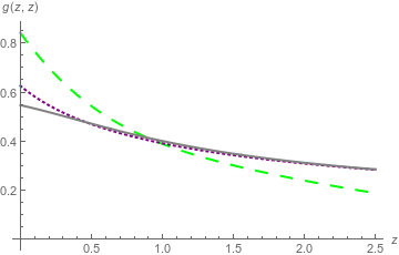
Figure 12: (color online) $g_{\kappa}(z,z)$ for $\alpha=1$ and $\kappa=0.8$. The solid gray line is the exact solution, the long-dashed green line is the perturbation expansion, and the dotted purple line is the WKB approximation. The perturbation expansion is very poor here, but the WKB expansion quickly converges to a reasonable value.

Ultimately, there is no reason why the approximation used for $F(z)$ and $G(z)$ must be the same as that used for $\gamma_{+}\,$, which implicitly involves $z=0$, since the location of the transition to WKB behavior depends on $z$.

VI Conclusion

The power wall is a promising model of the effects of a boundary on the vacuum state of a quantum field. It helps to separate the genuine effects from the pathologies associated with idealized boundary conditions.

This paper deals with a flat wall interacting with a scalar field. We have set up a systematic notation for the solutions of the separated field equation and developed useful approximations for them in the limits of large and small imaginary wavenumber $\kappa$, which have been tested numerically. In the region outside the wall, we obtained approximations for the energy density that closely match the exact solutions in both asymptotic limits and are reasonably accurate in between.

Progress in the region inside the wall has been slow, because of both technical problems and the conceptual complication of renormalization in the presence of a nontrivial potential. The renormalization problem has been investigated separately MNS ; self for a general potential; self uses higher-order WKB approximations, with special attention to the application to the power wall. Precise calculation of the renormalized stress tensor, including contributions from the non-WKB region of the spectrum, are in process.

The foremost motivation for this work was to resolve the “pressure anomaly” in the force on a perpendicular wall that has been observed Estrada-Mera in calculations for a hard wall regularized by a finite cutoff. Outside the soft wall, we have calculated the energy and pressure and shown that the anomaly does not occur in this model. (Eventual success inside the wall is expected.) We attribute this success to the fact that the soft-wall model is a consistent physical system whose energy density is well behaved from the start, rather than being forced to be finite by an ad hoc cutoff.

Calculations so far (here and in HSW ; thesis ; self ) deal primarily with small values of $\alpha$ and hence with the extraneous divergences near $z=0$ caused by the singularity in the potential there. For very large values of $\alpha$ these divergences must disappear, and the stress tensor must resemble that of a hard wall near $z=1$. Until such computations are available, it is not meaningful to make a comparison of our results with others, such as those of Barton or Passante et al. (see Appendix).

Appendix A Historical perspective

First to base the analysis of the Casimir effect on local quantities (i.e., the expectation values of components of the stress tensor) rather than total energy or force were Brown and Maclay BmC . DeWitt dewitt recognized the importance of this topic for understanding quantum field theory in curved space-time. Consequently, the generic behavior of the stress tensor near boundaries was investigated from differing points of view by two groups in Austin DC ; KCD ; Deutsch and Candelas DC argued that divergences in the total energy are related to finite and physically meaningful, though nonintegrable, distributions of energy density near the boundary and, therefore, must be taken seriously. This can be regarded as the origin of the modern program of softening (not discarding) surface terms by improved modeling of the boundaries themselves. Later, the analysis of the energy in a box in terms of classical paths by Hertzberg et al. HJKS demonstrated that energy density near boundaries has physical meaning and can be responsible for counterintuitive signs in some parts of Casimir forces.

One of the most ambitious programs in the direction of improved modeling has been conducted by Barton barton01 ; barton04a ; barton04b ; BartonB ; barton05b , studying nonlinear interactions of the field with degrees of freedom inside the walls.

Closer to the spirit of the present work is Ford and Svaiter’s investigation of a hard boundary whose location is subjected to random fluctuations FS . Similar work has been done recently by Passante et al. pas1 ; pas2 ; pas3

Qualitatively similar results appear in a large number of papers by Graham, Jaffe, Olum, and coworkers (such as Refs. GJKQSW ; OG ; GO ; Jaffe ) culminating in the book GQW . That program differs from ours superficially by dealing with a high, narrow potential hill (instead of a one-sided wall), and more fundamentally in the choice of calculational methods (techniques of scattering theory instead of local, differential-equation analyses), which results in a rather different point of view. An earlier paper in that tradition is Bordag bordag .

The present program is rooted in rect , which proposed to model a soft wall simply by maintaining a finite ultraviolet cutoff in calculations for a hard wall. Results were qualitatively so similar to those of Ford and Svaiter FS and Graham and Olum OG ; GO as to suggest that all the approaches were on the same track. However, in calculations for a spherical boundary, Martin Schaden and Fulling (unpublished, but summarized in norman09 ) discovered a pressure anomaly — a violation of Eq. (1). Detailed examination Estrada-Mera ; Benasque showed that this problem existed for flat boundaries also, and that it was related to the direction dependence of vacuum energy as regularized by point-splitting christensen . That is the motivation for the study of the soft wall SpecGeom ; HSW ; Benasque ; thesis ; self .

The closest work to ours that we know of in previous literature (until HSW and MNS ) is that of Actor and Bender AB , in which the perfectly reflecting wall is replaced by a harmonic-oscillator potential. That paper was written before the modern critiques of formal renormalization BartonA ; Jaffe and the modern emphasis on local quantities (such as energy density). It deals with total energies calculated by zeta-function regularization.

Here we have not reviewed papers on scalar quantum field theory in general background scalar potentials and the resulting issues of renormalization, since that topic relates more to self and possible later papers. Nor have we listed the large body of papers on fields interacting with slabs of material (such as dielectrics) or delta-function potentials; such models are not truly “soft” by our definition, since boundary divergences remain. The remarks on the works of Graham et al. and Actor and Bender are paraphrased from Benasque .

References

- (1) K. A. Milton, The Casimir Effect: Physical Manifestations of Zero-Point Energy (World Scientific, Singapore, 2001).
- (2) M. Bordag, G. L. Klimchitskaya, U. Mohideen, V. M. Mostepanenko, Advances in the Casimir Effect, International Series of Monographs on Physics 145 (Oxford U. Press, Oxford, 2009).
- (3) D. Dalvit, P. Milonni, D. Roberts, and F. da Rosa, Casimir Physics, Lecture Notes in Physics 834 (Springer, Berlin, 2011).
- (4) E. Elizalde, J. Phys. A 27, L299 (1994).
- (5) G. Barton, Internat. J. Mod. Phys. 17, 767 (2002).
- (6) R. L. Jaffe, in Quantum Field Theory Under the Influence of External Conditions, QFEXT’03, edited by K. A. Milton (Rinton Press, Princeton, 2004), pp. 175–185.
- (7) M. Schaden, Phys. Rev. A 73, 042102 (2006).
- (8) G. Barton, J. Phys. A 38, 2997 (2005).
- (9) S. A. Fulling, L. Kaplan, K. Kirsten, Z. H. Liu, and K. A. Milton, J. Phys. A 42, 155402 (2009).
- (10) K. A. Milton, Phys. Rev. D 84, 065028 (2011).
- (11) S. A. Fulling, Internat. J. Mod. Phys. A 25, 2364 (2010)
- (12) R. Estrada, S. A. Fulling, and F. D. Mera, J. Phys. A 45, 455402 (2012).
- (13) S. A. Fulling, F. D. Mera, and C. S. Trendafilova, Phys. Rev. D 87, 047702 (2013).
- (14) S. A. Fulling, K. A. Milton, and J. Wagner, Internat. J. Mod. Phys. A 27, 1260009 (2012).
- (15) J. D. Bouas, S. A. Fulling, F. D. Mera, K. Thapa, C. S. Trendafilova, and J. Wagner, in Spectral Geometry, edited by A. H. Barnett et al., Proceedings of Symposia in Pure Mathematics 84 (American Mathematical Society, Providence, 2011), pp. 139–154.
- (16) Colin Whisler and Steven Murray, The Soft Wall Model of the Casimir Effect, Undergraduate Research Scholar thesis, Texas A&M University, 2015; http://hdl.handle.net/1969.1/154485
- (17) M. Abramowitz and I. A. Stegun, editors, Handbook of Mathematical Functions …, Applied Mathematics Series 55 (National Bureau of Standards, Washington, 1964).
- (18) K. A. Milton, K. V. Shajesh, S. A. Fulling, and P. Parashar, Phys. Rev. D 89, 064027 (2014).
- (19) S. M. Christensen, Phys. Rev. D 14, 2490 (1976).
- (20) K. A. Milton, F. Kheirandish, P. Parashar, E. K. Abalo, S. A. Fulling, J. D. Bouas, H. Carter, and K. Kirsten, Phys. Rev. D 88, 025039 (2013).
- (21) G. Plunien, B. Müller, and W. Greiner, Phys. Reports 134, 87 (1986).
- (22) Ya. B. Zel’dovich, Sov. Phys. Usp. 11, 381 (1968) [Usp. Fiz. Nauk 95, 209].
- (23) S. M. Christensen, Phys. Rev. D 17, 946 (1978).
- (24) S. L. Adler, J. Lieberman, and Y. J. Ng, Ann. Phys. 106, 279 (1977).
- (25) F. D. Mazzitelli, J. P. Nery, and A. Satz, Phys. Rev. D 84, 125008 (2011).
- (26) F. D. Mera, S. A. Fulling, J. D. Bouas, and K. Thapa, J. Phys. A 46, 195302 (2013).
- (27) K. A. Milton, S. A. Fulling, P. Parashar, P. Kalauni, and T. Murphy, arXiv:1602.00916.
- (28) L. S. Brown and G. J. Maclay, Phys. Rev. 184, 1272 (1969).
- (29) B. S. DeWitt, Phys. Reports 19, 295 (1975).
- (30) D. Deutsch and P. Candelas, Phys. Rev. D 20, 3063 (1979).
- (31) G. Kennedy, R. Critchley, and J. S. Dowker, Ann. Phys. (NY) 125, 346 (1980).
- (32) M. P. Hertzberg, R. L. Jaffe, M. Kardar, and A. Scardicchio, Phys. Rev. Lett. 95, 250402 (2005).
- (33) G. Barton, J. Phys. A 34, 4083 (2001).
- (34) G. Barton, J. Phys. A 37, 1011 (2004).
- (35) G. Barton, J. Phys. A 37, 3725 (2004).
- (36) G. Barton, J. Phys. A 38, 3021 (2005).
- (37) L. H. Ford and N. F. Svaiter, Phys. Rev. D 58, 065007 (1998).
- (38) S. Butera and R. Passante, Phys. Rev. Lett. 111, 060403 (2013).
- (39) N. Bartolo, S. Butera, M. Lattuca, R. Passante, L. Rizzuto, and S. Spagnolo, J. Phys. Cond. Mat. 10, 27 (2014).
- (40) A. Armata and R. Passante, Phys. Rev. D 91, 025012 (2015).
- (41) N. Graham, R. L. Jaffe, V. Khemani, M. Quandt, M. Scandurra, and H. Weigel, Nucl. Phys. B 645, 49 (2002).
- (42) K. D. Olum and N. Graham, Phys. Lett. B 554, 175 (2003).
- (43) N. Graham and K. D. Olum, Phys. Rev. D 67, 085014 (2003).
- (44) N. Graham, M. Quandt, and H. Weigel, Spectral Methods in Quantum Field Theory, Lec. Notes in Phys. 777 (Springer-Verlag, Heidelberg, 2009).
- (45) M. Bordag, J. Phys. A 28, 755 (1995).
- (46) A. Actor and I. Bender, Phys. Rev. D 52, 3581 (1995).