Limiting Eigenvalue Distribution of Random Matrices of Ihara Zeta Function of Long-Range Percolation Graphs

Abstract

We consider the ensemble of $N\times N$ real random symmetric matrices $H_{N}^{(R)}$ obtained from the determinant form of the Ihara zeta function associated to random graphs $\Gamma_{N}^{(R)}$ of the long-range percolation radius model with the edge probability determined by a function $\phi(t)$.

We show that the normalized eigenvalue counting function of $H_{N}^{(R)}$ weakly converges in average as $N,R\to\infty$, $R=o(N)$ to a unique measure that depends on the limiting average vertex degree of $\Gamma_{N}^{(R)}$ given by $\phi_{1}=\int\phi(t)dt$. This measure converges in the limit of infinite $\phi_{1}$ to a shift of the Wigner semi-circle distribution. We discuss relations of these results with the properties of the Ihara zeta function and weak versions of the graph theory Riemann Hypothesis.

1 Introduction: Ihara zeta function and random matrices

The Ihara zeta function introduced by Y. Ihara in the algebraic context [14] attracts considerable interest also due to its interpretations in the frameworks of graph theory. Given a finite connected non-oriented graph $\Gamma=(V,E)$ with the vertex set $V=\{\alpha_{1},\alpha_{2},\dots,\alpha_{N}\}$ and the edge set $E$, the Ihara zeta function (IZF) of $\Gamma$ is defined for $u\in{\mathbb{C}}$ with $|u|$ sufficiently small, by

$$Z_{\Gamma}(u)=\prod_{[C]}\ (1-u^{\nu(C)})^{-1},$$

where the product runs over the equivalence classes of primitive closed backtrackless, tailless paths $C=(\alpha_{i_{1}},\alpha_{i_{2}},\dots,\alpha_{i_{l-1}},\alpha_{i_{l}})$, $\alpha_{i_{l}}=\alpha_{i_{1}}$ of positive length $l$ such that $\{\alpha_{i_{h}},\alpha_{i_{h+1}}\}\in E$ for all $h=1,\dots,l-1$ and $\nu(C)=l-1$ [29]. Here and below we denote by $e=\{\alpha_{i},\alpha_{j}\}$ a non-oriented edge $e\in E$ if it exists. In this definition (1.1), a closed path $C=(\alpha_{i_{1}},\alpha_{i_{2}},\dots,\alpha_{i_{l-1}},\alpha_{i_{1}})$ is primitive if there is no smaller path $\tilde{C}$ such that $C=\tilde{C}^{k}$. The path $C$ is backtrackless if $\alpha_{i_{h-1}}\neq\alpha_{i_{h+1}}$ for all $h=2,\dots,l-1$. The closed path $C$ is tailless if $\alpha_{i_{2}}\neq\alpha_{i_{l-1}}$. The equivalence class of closed paths $[C]$ includes $C$ and all paths obtained with the help of the cyclic permutations of its elements, i. e. of the form $C^{\prime}=(\alpha_{i_{2}},\dots,\alpha_{i_{l-1}},\alpha_{i_{1}},\alpha_{i_{2}})$, $C^{\prime\prime}=(\alpha_{i_{3}},\dots,\alpha_{i_{l-1}},\alpha_{i_{1}},\alpha_{i_{2}},\alpha_{i_{3}})$, etc. Let us note that the closed primitive backtrackless tailless paths can be imagined as analogs of the closed geodesics on manifolds. In this sense the absence of backtracking can be considered as the absence of singular (non-differentiable) points and the property to be tailless is analogous to differentiability of the geodesics at the origin.

The Ihara zeta function can also be expressed as

$$Z_{\Gamma}(u)=\exp\left\{\sum_{k\geq 1}{{\cal N}_{k}\over k}u^{k}\right\},$$

where ${\cal N}_{k}$ is the number of all classes of backtrackless tailless paths of the length $k$. Ihara’s theorem [14] says that the IZF (1.1) is the reciprocal of a polynomial and that for sufficiently small $|u|$

$$Z_{\Gamma}(u)^{-1}=(1-u^{2})^{r-1}\,\hbox{det}(I+u^{2}(B-I)-uA),$$

where $A=(a_{ij})_{i,j=1,\dots,N}$ is the adjacency matrix of ${\Gamma}$, $N$ is the number of vertices, $N=\#V$, $B=diag(\sum_{j=1}^{N}a_{ij})_{i=1,\dots,N}$ and $r-1={\mathrm{\,Tr}}(B-2I)/2$. Relation (1.3) proved by Y. Ihara firstly for the families of regular graphs that have the constant vertex degree, $\deg(\alpha_{i})=\deg(\alpha_{j})$, $i,j=1,\dots,N$ has been then generalized to the case of possibly irregular finite graphs where the degrees of different vertices may be different (see e.g. papers [2, 26] for the proofs on the basis of representation (1.2)).

At present, IZF is a well established part of the combinatorial graph theory with applications in number theory and spectral theory (see e.g. [13, 29] and references therein); it has also been studied in various other aspects, in particular in relations with the heat kernels on graphs [7], quantum walks on graphs [24], certain theoretical physics models [32]. Relations between the Ihara zeta function and spectral theory is a source of new interesting questions and problems.

While the Ihara’s determinant formula (1.3) gives a powerful tool in the studies of the Ihara zeta function, the explicit form of $Z_{\Gamma}(u)$ can be computed for relatively narrow families of finite graphs. The definition of the IZF associated to infinite graphs requires a number of additional restrictions and assumptions (see, in particular, [8, 11, 12, 20]). In the most studied cases, the graphs under consideration have a bounded vertex degree (in particular, regular or essentially regular graphs).

A complementary approach is related with the probabilistic point of view, when graphs are chosen at random from the family of all possible graphs on $N$ vertices. Such a description naturally leads to the limiting transition of infinitely increasing dimension of the graphs, $N\to\infty$. Certain aspects of zeta functions of large random regular graphs with finite vertex degree have been studied in [10].

Another class of random graphs is represented by the Erdős-Rényi ones [5]. This family of graphs $\{{\Gamma}_{N}^{(p)}\}$ can be described by the ensemble of real symmetric adjacency $N\times N$ matrices $A_{N}^{(p)}$ whose entries above the diagonal are given by jointly independent Bernoulli random variables with the average value $p$. In this model, the vertex degree is a random variable with the average value $pN$ that can be either finite or not in the limit $N\to\infty$.

In paper [16] we considered the eigenvalue distribution of random matrix ensemble obtained from the determinant formula (1.3) with the help of the adjacency matrices $A_{N}^{(\rho/N)}$ of the Erdős-Rényi random graphs. It is shown that after a proper renormalization of the spectral parameter $u$ by $\rho^{-1/2}$, this eigenvalue distribution converges in the limit $N,\rho\to\infty$ when $\rho=o(N^{\alpha})$ for any $\alpha>0$ to a shift of the widely known semi-circle Wigner distribution.

In the present paper we consider similar questions for random matrices related with random long-range percolation radius graphs [4, 25, 31], where the edge probability is a function of a kind of the distance between sites (vertices). These graphs can be thought as a generalization of the Erdős-Rényi ensemble that give somewhat better description of certain systems of interacting particles. Our main observation is that in the limit of infinite graph dimension and infinite interaction radius, the moments of the limiting eigenvalue distribution of the random matrix ensemble generated by the determinant formula (1.3) for random long-range percolation graphs verify a system of explicit relations in the case when the average vertex degree $\phi_{1}$ remains finite. Regarding the additional limiting transition $\phi_{1}\to\infty$, we obtain convergence of the limiting distribution to the same shifted semi-circle Wigner law as described in [16].

Let us consider the ensemble of $N\times N$ real symmetric matrices $A_{N}^{(R)}$,

$$\left(A_{N}^{(R,\phi)}\right)_{xy}=a_{xy}^{(R,\phi)},\quad|x|\leq n,\ |y|\leq n,\ N=2n+1,\ R\geq 1$$

whose entries above the main diagonal are given by a family of jointly independent Bernoulli random variables ${\cal A}^{(R,\phi)}=\{a^{(R,\phi)}_{xy},\ x,y\in{\mathbb{Z}},\ x\leq y\}$, such that

$$a^{(R,\phi)}_{xy}=\begin{cases}1-\delta_{x,y},&\text{with probability ${1\over R}\phi\left({x-y\over R}\right)=p_{R}\,$},\\ 0,&\text{with probability $1-{p_{R}}\,$,}\end{cases}$$

where $\delta_{x,y}$ is the Kronecker $\delta$-symbol. Then the matrix obtained is symmetrized to get (1.4). We assume that $\phi(t),t\in{\mathbb{R}}$ is a real continuous even function such that $0<\phi(t)<1$ and

$$\phi_{1}=\int_{{\mathbb{R}}}\phi(t)dt<+\infty\,.$$

We assume for simplicity that $\phi(t)$ is strictly decreasing for all $t\geq 0$. In what follows, we omit the superscripts $R$ and $\phi$ in $A_{N}^{(R,\phi)}$, ${\cal A}^{(R,\phi)}$ and $a_{xy}^{(R,\phi)}$ everywhere when no confusion can arise.

The ensemble of random graphs $\{{\Gamma}_{N}^{(R)}\}$ determined by the adjacency matrices $A_{N}^{(R)}$ (1.3) is close to the well-known ensemble of random long-range percolation radius graphs [A, 4, 25, 31]. In certain cases one considers graphs that have a number of non-random edges. We do not add to the graphs the non-random edges and assume that there are no loops in ${\Gamma}$. To generalize the existing models, we introduce the additional parameter $R$ into the definition of the edge probability $p_{R}$ that has not been used in the long-range percolation models cited above.

We introduce the diagonal matrix

$$\left(B_{N}^{(R)}\right)_{xt}=\delta_{x,t}\ \sum_{y=-n}^{n}a^{(R)}_{xy},\quad|x|,|t|\leq n,$$

and consider the logarithm of the Ihara zeta function of ${\Gamma}_{N}^{(R)}$,

$$-{1\over N}\log Z_{{\Gamma}_{N}^{(R)}}(u)={1\over 2N}{\mathrm{\,Tr}}\left(B_{N}^{(R)}-2I\right)\log(1-u^{2})$$

$$+{1\over N}\log\hbox{det}\left(I(1-u^{2})+u^{2}B_{N}^{(R)}-uA_{N}^{(R)}\right).$$

Regarding the first term of the right-hand side of (1.8)

$$\Upsilon_{N}^{(R)}={1\over 2N}{\mathrm{\,Tr}}(B_{N}^{(R)}-2I)\log(1-u^{2}),$$

it is easy to compute its mathematical expectation ${\bf\,E}\Upsilon_{N}^{(R)}$ with respect to the measure generated by the family ${\cal A}^{(R)}$,

$${\bf\,E}\Upsilon_{N}^{(R)}=\left({1\over 2NR}\sum_{x,t=-n}^{n}\phi\left({x-t\over R}\right)-{1\over 2R}\phi(0)-1\right)\log(1-u^{2}).$$

In present paper we consider the asymptotic regime of large $N$ and $R$

$$N\to\infty,\ R\to\infty,\ R=o(N)$$

that we denote by $(N,R)^{\circ}\to\infty$. It follows from (1.6) and (1.9) that

$$\lim_{(N,R)^{\circ}\to\infty}{\bf\,E}\Upsilon_{N}^{(R)}=\left({\phi_{1}\over 2}-1\right)\log(1-u^{2}).$$

and therefore it is natural to consider a rescaling of the parameter $u$ given by

$$u={v\over\sqrt{\phi_{1}}}.$$

Let us note that $\phi_{1}$ represents the average vertex degree of ${\Gamma}_{N}^{(R)}$ in the limit (1.10).

Taking into account (1.12), we rewrite the last term of (1.8) as

$$\Psi_{N}^{(R)}={1\over N}\log\hbox{det}\left(\left(1-{v^{2}\over\phi_{1}}\right)I+H_{N}^{(R)}(v)\right),$$

where

$$H_{N}^{(R)}(v)={v^{2}\over\phi_{1}}B_{N}^{(R)}-{v\over\sqrt{\phi_{1}}}A_{N}^{(R)}=\tilde{B}_{N}^{(R)}-\tilde{A}_{N}^{(R)}.$$

The main goal of the present paper is to study the limiting eigenvalue distribution of these random matrices with real $v$. Up to our knowledge, the random matrix ensemble $\{H_{N}^{(R)}(v)\}$ is a new one. It arises from the determinant formula for the Ihara zeta function (1.3) with a particular choice of the renormalization of the spectral parameter (1.12) determined by the asymptotic expression of the factor $(1-u)^{r-1}$. As far as we know, the limiting spectral properties of random matrices (1.14) have not yet been studied.

2 Eigenvalue counting function of random matrices

Let us denote the eigenvalues of the real symmetric matrix $H_{N}^{(R)}(v)$, $v\in{\mathbb{R}}$ by $\lambda_{1}\leq\dots\leq\lambda_{N}$. We consider the normalized eigenvalue counting function,

$$\sigma_{N,R}(\lambda)={1\over N}\sum_{j:\,\lambda_{j}\leq\lambda}1,$$

and denote by ${\bf\,E}\sigma_{N,R}=\bar{\sigma}_{N,R}$ its average with respect to the measure generated by ${\cal A}^{(R)}$. The measure $\bar{\sigma}_{N,R}$ can be characterized by its moments,

$$M_{k}^{(N,R)}=\int_{{\mathbb{R}}}\,\lambda^{k}d\bar{\sigma}_{N,R}(\lambda)={1\over N}{\bf\,E}{\mathrm{\,Tr}}\left(H_{N}^{(R)}\right)^{k}.$$

The main result of the present paper is as follows.

Theorem 2.1. Given $k\in{\mathbb{N}}$, the moment (2.1) converges in the limit (1.10) to $m_{k}^{(v,\phi_{1})}$,

$$\lim_{(N,R)^{\circ}\to\infty}M_{k}^{(N,R)}=m_{k}^{(v,\phi_{1})}.$$

This limiting moment $m_{k}^{(v,\phi_{1})}$ is given by relation

$$m_{k}^{(v,\phi_{1})}=\sum_{r=1}^{k}\Theta(k,r),$$

where the family $\{\Theta(k,r),\ 1\leq r\leq k\}_{k\in{\mathbb{N}}}$ is determined by the following recurrence,

$$\Theta(k,r)=\ \sum_{g=1}^{r}\ \sum_{s=r-g}^{k-g}{r-1\choose g-1}\,\Theta(s,r-g)$$

$$\times\ \sum_{w=0}^{g}\ \ \sum_{h=0}^{k-s-g-w}\ \ \sum_{t=0}^{k-s-g-w-h}\ \ {v^{2(g+h)}\over\phi_{1}^{g+h-1}}\ {g\choose w}\,$$

$$\times\ {w+h-1\choose h}^{*}\ {w+h+t-1\choose t}^{*}\ \Theta(k-s-g-w-h,t),$$

with the initial conditions $\Theta(k,0)=\delta_{k,0},\ k\geq 0.$ In (2.4), the generalized binomial coefficient is such that

$${i-1\choose i}^{*}=\delta_{i,0},\quad i=0,1,2,\dots.$$

It should be pointed out that relations similar to (2.4) have been obtained in our previous work [17] (see also [3, 18]) for similar but different ensemble of random matrices. In papers [17, 18] we studied the limiting eigenvalue distribution of the discrete analog of the Laplace operator of the Erdős-Rényi ensemble of random graphs. This discrete analog has been normalized by $\rho^{-1/2}$, where $\rho/n$ represents the edge probability of the random $n$-dimensional graphs. Due to this difference in the normalization factor, random matrices $H_{N}^{(R)}(v)$ we consider here are no more positive definite. In consequence, relations (2.4) differ from those obtained in [17] as well as the limiting eigenvalue distribution obtained after the transitions $\phi_{1}\to\infty$ and $\rho\to\infty$, respectively.

The mathematical expectation of the right-hand side of (2.1)

$${\bf\,E}{\mathrm{\,Tr}}(H^{k})={1\over N}\sum_{x_{1},x_{2},\dots,x_{n}}{\bf\,E}\left(H_{x_{1}x_{2}}H_{x_{2}x_{3}}\cdots H_{x_{k-1}x_{1}}\right)$$

can be considered as a sum over the set of weighted closed walks of $k$ steps $(x_{1},\dots,x_{k-1},x_{1})$. This interpretation proposed in the pioneering works by E. Wigner (see e. g. [30]) has been used, in one or another form, in a large number of papers on random matrix theory. We follow this strategy to study the product

$${\cal S}^{(N,R)}_{(\bar{p},\bar{q})}(s)={1\over N}\sum_{x_{1}=-n}^{n}\cdots\sum_{x_{s}=-n}^{n}\ {\bf\,E}\left(\tilde{A}^{p_{1}}_{x_{1}x_{2}}\,\tilde{B}^{q_{1}}_{x_{2}x_{2}}\tilde{A}^{p_{2}}_{x_{2}x_{3}}\cdots\tilde{B}^{q_{s-1}}_{x_{s}x_{s}}\tilde{A}^{p_{s}}_{x_{s}x_{1}}\tilde{B}^{q_{s}}_{x_{1}x_{1}}\right),$$

where the numbers $p_{i},q_{j}$ are such that

$$p_{1}\geq 0,p_{i}>0,i=2,\dots,s,\ q_{s}\geq 0,q_{j}>0,j=1,\dots,s-1,\ P+Q=k,$$

where $P=\sum_{i=1}^{s}p_{i}$ and $Q=\sum_{i=1}^{s}q_{i}$. It is clear that we can rewrite (2.1) as follows,

$$M_{k}^{(N,R)}=\sum_{s=1}^{k}\ \sum_{(\bar{p},\bar{q})^{*}}^{k}(-1)^{P}{\cal S}^{(N,R)}_{(\bar{p},\bar{q})}(s),$$

where $\bar{p}=(p_{1},p_{2},\dots,p_{s})$, $\bar{q}=(q_{1},q_{2}\dots,q_{s})$, and the star in the last sum means that it runs over all $(\bar{p},\bar{q})$ from (2.6).

2.1 Color diagrams and weights

Let us consider the set of variables of the summation of (2.6)

$$\bar{x}_{\bar{p}}^{(s)}=\left\{\left(x_{i}^{(1)},\dots,x_{i}^{(p_{i})},x_{i}^{(p_{i}+1)}\right)\right\}_{i=1}^{s}\ {\hbox{and}}\ \ \bar{y}_{\bar{q}}^{(s)}=\left\{\left(y_{j}^{(1)},\dots,y_{j}^{(q_{j})}\right)\right\}_{j=1}^{s},$$

where $x^{(1)}_{i}=x_{i}$, $x_{i}^{(p_{i}+1)}=x_{i+1}=x_{i+1}^{(1)}$, $i=1,\dots,s$ and $x_{s}^{(p_{s}+1)}=x_{s+1}=x_{1}$ such that

$$\tilde{A}^{p_{i}}_{x_{i}x_{i+1}}=\left({v\over\sqrt{\phi_{1}}}\right)^{p_{i}}\sum_{x_{i}^{(2)},\dots,x_{i}^{(p_{i})}}\ a_{x_{i}^{(1)}x_{i}^{(2)}}\,a_{x_{i}^{(2)}x_{i}^{(3)}}\,\cdots\,a_{x_{i}^{(p_{i})}x_{i}^{(p_{i}+1)}}$$

and

$$\tilde{B}^{q_{j}}_{x_{j+1}x_{j+1}}=\left({v^{2}\over{\phi_{1}}}\right)^{q_{j}}\sum_{y_{j}^{(1)},\dots,y_{j}^{(q_{j})}}a_{x_{j+1}y_{j}^{(1)}}\,a_{x_{j+1}y_{j}^{(2)}}\,\cdots\,a_{x_{j+1}y_{j}^{(q_{j})}},\quad j=1,\dots,s.$$

Then can we rewrite the right-hand side of (2.6) as follows,

$${1\over N}\sum_{x_{1}=-n}^{n}\cdots\sum_{x_{s}=-n}^{n}{\bf\,E}\left(\tilde{A}^{p_{1}}_{x_{1}x_{2}}\,\tilde{B}^{q_{1}}_{x_{2}x_{2}}\tilde{A}^{p_{2}}_{x_{2}x_{3}}\cdots\tilde{B}^{q_{s-1}}_{x_{s}x_{s}}\tilde{A}^{p_{s}}_{x_{s}x_{1}}\tilde{B}^{q_{s}}_{x_{1}x_{1}}\right)$$

$$={1\over N}\sum_{x_{1}=-n}^{n}\cdots\sum_{x_{s}=-n}^{n}\ \prod_{i=1}^{s}\ \sum_{x_{i}^{(2)},\dots,x_{i}^{(p_{i})}}\ \ \prod_{j=1}^{s}\ \sum_{y_{j}^{(1)},\dots,y_{j}^{(q_{j})}}\left({v\over\sqrt{\phi_{1}}}\right)^{P+2Q}$$

$$\times{\bf\,E}\left(a_{x_{i}x_{i}^{(2)}}\,a_{x_{i}^{(2)}x_{i}^{(3)}}\,\cdots\,a_{x_{i}^{(p_{i})}x_{i+1}\textdagger}\cdot a_{x_{j+1}y_{j}^{(1)}}\,a_{x_{j+1}y_{j}^{(2)}}\,\cdots\,a_{x_{j+1}y_{j}^{(q_{j})}}\right).$$

Regarding the product of random variables of (2.8), we cannot say do they represent the independent ones or not; therefore we cannot compute the mathematical expectation until concrete values taken by variables $x$ and $y$ are known. Given these concrete values that we denote by $\langle x\rangle$ and $\langle y\rangle$, we can use the fundamental property that the random variables $a_{\langle x\rangle\langle y\rangle}$ and $a_{\langle x^{\prime}\rangle\langle y^{\prime}\rangle}$ (1.5) are independent and all their mixed moments factorize unless either $\langle x\rangle=\langle x^{\prime}\rangle$ and $\langle y\rangle=\langle y^{\prime}\rangle$ or $\langle x\rangle=\langle y^{\prime}\rangle$ and $\langle y\rangle=\langle x^{\prime}\rangle$. We are going to develop a diagram technique that helps to compute the mathematical expectation of (2.8) for any given particular realization of variables $\bar{x}_{\bar{p}}^{(s)}$ and $\bar{y}_{\bar{q}}^{(s)}$. Using these diagrams, we can separate the set of all such realizations into the classes of equivalence and to evaluate the sum over those classes that give non-vanishing contribution to the sum (2.8) in the limit $(N,R)^{\circ}\to\infty$.

The diagram technique we develop is not completely new. We are based on the approach proposed in papers [17, 18] to study the moments of the discrete version of the Laplace operator for large random Erdős-Rényi graphs. However, the fact that the edge probability of $e=\{x,y\}$ depends on the difference $x-y$ (1.5) requires a number of essential modifications of the method of [17, 18]. The main idea here is to describe a kind of multigraph such that its edges represent independent random variables and such that the multiplicities of the multi-edges take into account the number of times that given random variable appears in the product (2.8). We refer to these multigraphs as to the diagrams. Their structure is fairly natural and intuitively clear (see examples presented below on Figures 1 and 2), while the formal description of their construction is somehow cumbersome. Let us pass to rigorous definitions.

2.1.1 Color diagrams

Given $\bar{p}$, $\bar{q}$ and regarding the family of variables $(X_{\bar{p}},Y_{\bar{q}})=(\bar{x}_{\bar{p}}^{(s)},\bar{y}_{\bar{q}}^{(s)})$ of the right-hand side of (2.8), we denote by

$$\langle X_{\bar{p}},Y_{\bar{q}}\rangle_{n}=\langle\bar{x}_{\bar{p}}^{(s)},\bar{y}_{\bar{q}}^{(s)}\rangle_{n}$$

a particular realization of $(X_{\bar{p}},Y_{\bar{q}})$ that attributes to each variable an integer from $\{-n,\dots,n\}$ and construct by recurrence a diagram ${\cal D}_{k}(\langle X_{\bar{p}},Y_{\bar{q}}\rangle_{n})$ that is a multigraph with $k$ oriented edges that we denote by $e_{i},i=1,\dots,k$. To simplify denotations, we will omit the subscripts and arguments in ${\cal D}$ when no confusion can arise. We denote the set of edges of ${\cal D}$ by ${\cal E}$ and the set of vertices of ${\cal D}$ by ${\cal V}=\{\upsilon_{j},1\leq j\leq\kappa\}$. The diagram ${\cal D}=({\cal V},{\cal E})$ consists of two sub-diagrams: the blue one ${\cal D}^{(b)}$ with blue vertices and $P$ blue edges, and the red one ${\cal D}^{(r)}$ with red vertices and $Q$ red edges.

We construct ${\cal D}^{(b)}$ first. To do this, we consider the realization $\langle X_{\bar{p}}\rangle_{n}$ as an ordered sequence of $P+1$ integers denoted by ${\cal I}_{P+1}=(I_{1},I_{2},\dots,I_{P},I_{1})$, $I_{i}\in\{-n,\dots,n\}$. This order is naturally imposed by variables $x_{i}^{(j)}$ in the product of (2.6). We start the construction of ${\cal D}^{(b)}$ by drawing the vertex $u_{1}$; we attribute to it the integer $I_{1}=\langle x_{1}^{(1)}\rangle_{n}$. This is the first step of the recurrence that we will refer to as the $x$-recurrence.

If $p_{1}>0$, then the second integer $I_{2}$ is given by $\langle x_{1}^{(2)}\rangle_{n}$. If $p_{1}=0$, then $I_{2}=\langle x_{2}^{(2)}\rangle_{n}$. It follows from (1.5) that $a_{xx}^{(R)}=0$; to avoid the trivial case, we accept that $I_{2}\neq I_{1}$ and create the second vertex $u_{2}\neq u_{1}$. Then we attribute to $u_{2}$ the integer $I_{2}$ and draw the oriented edge $\epsilon_{1}=(u_{1},u_{2})$. We attribute to this edge the random variable $a_{I_{1}I_{2}}$. This terminates the second step of the $x$-recurrence, $t=2$.

To describe the general recurrence rule, we consider the ensemble ${\mathbb{U}}_{t}$ of vertices $u_{i}$ created during the first $t$ steps and denote $\varkappa_{t}=\#{\mathbb{U}}_{t}$, $t\geq 1$. We denote by ${\mathbb{I}}_{t}$ the set of integers attributed to the vertices of ${\mathbb{U}}_{t}$. We assume that all elements of ${\mathbb{I}}_{t}$ are different and ${\mathbb{I}}_{t}$ is in one-to-one correspondence with ${\mathbb{U}}_{t}$. These properties will be proved by construction during the $x$-recurrence procedure.

We take the next in turn integer $I_{t+1}$ not equal to $I_{t}$ due to (1.5) and perform the following actions:

- if there exists such $I^{\prime}\in{\mathbb{I}}_{t}$ that $I_{t+1}=I^{\prime}$, then we consider the already existing vertex $u^{\prime}=u(I^{\prime})$ attributed by $I^{\prime}$; this vertex is uniquely determined. Then we consider the vertex $\hat{u}=u(I_{t})$ attributed by $I_{t}$ and draw the edge $\epsilon_{t}=(\hat{u},u^{\prime})$. It is clear that in this case $\varkappa_{t+1}=\varkappa_{t}$. We attribute to this edge the random variable $a_{I_{t}I^{\prime}}$;

- if there is no such values $I^{\prime}\in{\mathbb{I}}_{t}$ that $I^{\prime}=I_{t+1}$, then we create a new vertex $u_{\varkappa_{t}+1}$, attribute to it $I_{t+1}$ and draw the edge $\epsilon_{t}=(\hat{u},u_{\varkappa_{t}+1})$, where $\hat{u}=u(I_{t})$. Obviously, $\varkappa_{t+1}=\varkappa_{t}+1$. We attribute to this edge the random variable $a_{I_{t}I_{t+1}}$.

We proceed till the last step $t+1=P+1$ is performed and the last edge $\epsilon_{P}=(u(I_{P}),u_{1})$ is drawn. We color all vertices of ${\mathbb{U}}_{P+1}$ and $P$ edges obtained in blue color. The sub-diagram ${\cal D}^{(b)}$ is constructed.

Now we describe the $y$-recurrence that adds to ${\cal D}^{(b)}$ the red elements of ${\cal D}$. Realization $\langle\bar{y}_{\bar{q}}^{(s)}\rangle$ can be considered as a chronologically ordered sequence of $Q$ integers ${\cal J}=(J_{1},\dots,J_{Q})$. We take the first integer $J_{1}=\langle y_{1}^{(1)}\rangle_{n}$ and compare it with the elements of ${\mathbb{I}}_{P}$. Taking into account (1.5), we assume that $J_{1}\neq I_{p_{1}+1}$. If there exists such $I^{\prime}\in{\mathbb{I}}_{P}$ that $J_{1}=I^{\prime}$, then we join the vertex $\hat{u}\in{\mathbb{U}}_{P}$ attributed by $I_{p_{1}+1}$, with the vertex $u^{\prime}$ attributed by $I^{\prime}$ by the edge $(\hat{u},u^{\prime})$ and color it in red. We attribute to this edge random variable $a_{I_{p_{1}+1}I^{\prime}}$. If there is no such $I^{\prime}$, then we create a new vertex $w_{1}$ that we color in red and draw the red edge $\varepsilon_{1}=(\hat{u},w_{1})$. We attribute to $w_{1}$ the value $J_{1}$ and attribute to $\varepsilon_{1}$ the random variable $a_{I_{p_{1}+1}J_{1}}$.

To describe the general step $\tau+1$ of $y$-recurrence, we introduce the set ${\mathbb{J}}_{\tau}$ of integers attributed to the set ${\mathbb{W}}_{\tau}$ of red vertices created during the first $\tau$ steps. We take $J_{\tau+1}$ and compare it with the elements of the set $\{{\mathbb{I}}_{P},{\mathbb{J}}_{\tau}\}={\mathbb{I}}_{P}\cup{\mathbb{J}}_{\tau}$.

- If there exists such $K^{\prime}\in\{{\mathbb{I}}_{P},{\mathbb{J}}_{\tau}\}$ that $J_{\tau+1}=K^{\prime}$, then we draw the red edge $\varepsilon_{\tau+1}=(\hat{u},v^{\prime})$, where $\hat{u}=u(I_{p_{1}+\dots+p_{j}+1})$ if $q_{1}+\dots+q_{j-1}+1\leq\tau\leq q_{1}+\dots+q_{j}$ and

$$v^{\prime}=\begin{cases}u^{\prime}=u(K^{\prime})\in{\mathbb{U}}_{P},&\text{if $K^{\prime}\in{\mathbb{I}}_{P}$},\\ w^{\prime}=w(K^{\prime})\in{\mathbb{W}}_{\tau},&\text{if $K^{\prime}\in{\mathbb{J}}_{\tau}$.}\end{cases}$$

In this case the cardinality $\varrho_{\tau}=\#{\mathbb{W}}_{\tau}$ does not change its value, $\varrho_{\tau+1}=\varrho_{\tau}$. We attribute to the edge $\varepsilon_{\tau+1}$ the random variable $a_{I_{p_{1}+\dots+p_{j}+1}K^{\prime}}$.

- If there is no such $K^{\prime}\in\{{\mathbb{I}}_{P},{\mathbb{J}}_{\tau}\}$ that $J_{\tau+1}=K^{\prime}$, then we create a new red vertex $w_{\varrho_{\tau}+1}$ and attribute $J_{\tau+1}$ to it. We also draw the red edge $\varepsilon_{\tau+1}=(\hat{u},w_{\varrho_{\tau}+1})$ and set ${\mathbb{J}}_{\tau+1}=\{{\mathbb{J}}_{\tau},J_{\tau+1}\}$. We attribute to the edge $\varepsilon_{\tau+1}$ the random variable $a_{I_{p_{1}+\dots+p_{j}+1}J_{\tau+1}}$. In all these considerations, we have assumed that $J_{\tau+1}\neq I_{p_{1}+\dots+p_{j}+1}$.

The last step of the $y$-recurrence is $\tau+1=Q$ and the red sub-diagram ${\cal D}^{(r)}$ is constructed. Let us point out that the total number of vertices $\nu=\#{\cal V}$ cannot be greater than $n$.

Finally, we get the diagram ${\cal D}=({\cal V},{\cal E})$ by renaming the edges of ${\cal D}^{(b)}\uplus{\cal D}^{(r)}$ by $(e_{1},e_{2},\dots,e_{k})$, $k=P+Q$ according to the data $(\bar{p},\bar{q})$. This means that the first $p_{1}$ edges $e_{1},\dots,e_{p_{1}}$ are the blue ones, then $e_{p_{1}+1},\dots,e_{p_{1}+q_{1}}$ are the red ones followed by $p_{2}$ blue edges $e_{p_{1}+q_{1}+1},\dots,e_{p_{1}+q_{1}+p_{2}}$, and so on. Finally, we rename the vertices of ${\cal D}^{(b)}\uplus{\cal D}^{(r)}$ by $(\upsilon_{1},\upsilon_{2},\dots,\upsilon_{\nu})$ according to the order of their appearance in the sequence of edges $(e_{1},e_{2},\dots,e_{k})$. The diagram ${\cal D}$ is constructed.

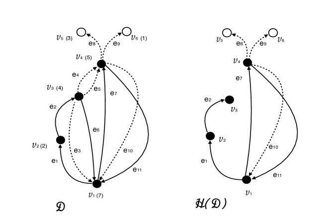
Figure 1: The diagram ${\cal D}$ and its sub-diagram ${\cal H}({\cal D})=\hat{\cal D}$

For example, taking $\bar{p}=(2,2,1)$, $\bar{q}=(3,3,0)$ and realization $\langle X_{\bar{p}},Y_{\bar{q}}\rangle_{9}$ such that

$${\cal I}=(7,2,4,7,5,7),\quad{\cal J}=(7,5,5,3,1,7),$$

we get a diagram ${\cal D}$ with six vertices, five blue edges $e_{1},e_{2},e_{6},e_{7},e_{11}$ and six red edges $e_{3},e_{4},e_{5},e_{8},e_{9},e_{10}$, where $e_{1}=\epsilon_{1}=(\upsilon_{1},\upsilon_{2})$, $e_{2}=\epsilon_{2}=(\upsilon_{2},\upsilon_{3})$, $e_{3}=\varepsilon_{1}=(\upsilon_{3},\upsilon_{1})$, $e_{4}=\varepsilon_{2}=(\upsilon_{3},\upsilon_{4})$ and so on. On Figure 1, we denoted by dotted lines and empty circles the red edges and red vertices, respectively. The numbers in parenthesis indicate the integers attributed to the vertices of ${\cal D}$. For simplicity, we have used in ${\cal I}$ and ${\cal J}$ positive integers only.

As one can see, the diagram ${\cal D}$ contains $P$ blue edges and $Q$ red ones. For any two vertices $\upsilon_{i}$ and $\upsilon_{j}$ joined by an edge of ${\cal D}$, we denote by ${\mathfrak{b}}(\{\upsilon_{i},\upsilon_{j}\})$ the total number of blue edges of the form $(\upsilon_{i},\upsilon_{j})$ and $(\upsilon_{j},\upsilon_{i})$ and by ${\mathfrak{r}}(\{\upsilon_{i},\upsilon_{j}\})$ the total number of red edges of the form $(\upsilon_{i},\upsilon_{j})$ and $(\upsilon_{j},\upsilon_{i})$.

Regarding a vertex $\upsilon\in{\cal V}({\cal D})$ such that $\upsilon\neq\upsilon_{1}$, one can find unique vertex $\upsilon^{\prime}$ such that $\upsilon$ has been created in ${\cal D}^{(b)}\uplus{\cal D}^{(r)}$ by arrival from $\upsilon^{\prime}$. Keeping all edges of ${\cal D}$ of the form $(\upsilon,\upsilon^{\prime})$ and $(\upsilon^{\prime},\upsilon)$ and erasing all other edges from ${\cal E}({\cal D})$, we will get a new diagram that is a sub-diagram of ${\cal D}$. We denote this sub-diagram by $\hat{\cal D}={\cal H}({\cal D})$ (see Figure 1).

Regarding the set of vertices ${\cal V}({\cal D})$, we can join each couple $\upsilon_{i},\upsilon_{j}$ such that ${\mathfrak{b}}(\{\upsilon_{i},\upsilon_{j}\})+{\mathfrak{r}}(\{\upsilon_{i},\upsilon_{j}\})>0$ by a non-oriented simple edge. Thus we get a graph $G=G({\cal D})$ such that ${\cal V}(G)={\cal V}({\cal D})$. We accept that the vertices of $G$ are ordered according to the order of elements of ${\cal V}({\cal D})$ and denote the set of ordered edges of $G$ by $E(G)$. Regarding $G(\hat{\cal D})$, we get a graph $\hat{G}$ that is a plane rooted tree with the root vertex $\upsilon_{1}$.

Having constructed the diagram ${\cal D}$, we define a generalized diagram ${\cal D}_{\xi}$ by attributing variables $\xi_{i},1\leq i\leq\nu$ to the vertices of ${\cal D}$ according to their order. In what follows, we denote the collection of these variables by $\bar{\xi}_{\nu}=(\xi_{1},\dots,\xi_{\nu})$. By the same way we determine the generalized graph $G_{\xi}$.

2.1.2 Weight of the diagram

By construction, random variables $a$ (1.5) attributed to different edges of $G({\cal D})$ are different and therefore they are jointly independent. Returning to the example realization $\langle X_{\bar{p}},Y_{\bar{q}}\rangle_{9}$ from above and considering the corresponding diagram ${\cal D}$ of Figure 1, we can easily find that the value of the average of the right-hand side of (2.8) is equal to the mathematical expectation

$${v^{11}\over\phi_{1}^{11/2}}{\bf\,E}\left(a^{(R)}_{72}a^{(R)}_{24}\left(a^{(R)}_{47}\right)^{2}\left(a^{(R)}_{45}\right)^{2}a^{(R)}_{53}a^{(R)}_{51}\left(a^{(R)}_{57}\right)^{3}\right)$$

that factorizes to the product of moments of seven random variables involved.

Regarding the generalized diagram ${\cal D}_{\xi}$, it is natural to attribute to each non-oriented edge $e=\{\upsilon_{i},\upsilon_{j}\}$ of $G({\cal D}_{\xi})=G_{\xi}$ the value

$$\pi_{e}^{(R)}(\bar{\xi}_{\nu})=\pi^{(R)}_{\{\upsilon_{i},\upsilon_{j}\}}(\bar{\xi}_{\nu})={\displaystyle v^{{\mathfrak{b}}(e)+2{\mathfrak{r}}(e)}\over\displaystyle\phi_{1}^{{\mathfrak{b}}(e)/2+{\mathfrak{r}}(e)}}\cdot{1\over R}\phi((\xi_{i}-\xi_{j})/R)$$

where $\xi_{i}$ and $\xi_{j}$ are given by the variables attributed to the vertices $\upsilon_{i}$ and $\upsilon_{j}$, respectively. Then the total weight of the generalized diagram is

$$\Pi^{(R)}({\cal D}_{\xi},\bar{\xi})=\prod_{e\in G_{\xi}}\pi^{(R)}_{\{\upsilon_{i},\upsilon_{j}\}}(\bar{\xi}_{\nu}).$$

Given $\bar{p}$ and $\bar{q}$ of (2.8), any realization of variables $\langle X_{\bar{p}},Y_{\bar{q}}\rangle_{n}$ generates a diagram ${\cal D}(\langle X_{\bar{p}},Y_{\bar{q}}\rangle_{n})$. We say that two realizations $\langle X_{\bar{p}},Y_{\bar{q}}\rangle_{n}^{\prime}$ and $\langle X_{\bar{p}},Y_{\bar{q}}\rangle_{n}^{\prime\prime}$ are equivalent, if their diagrams coincide. One should note that the value of the mathematical expectation (2.8) for these realizations can be different. From another hand, for any realization $\langle X_{\bar{p}},Y_{\bar{q}}\rangle_{n}$ a unique realization $\langle\bar{\xi}_{\nu}\rangle_{n}$ of the variables of ${\cal D}_{\xi}$ is determined; obviously, this realization is given by the values attributed to the vertices of ${\cal D}(\langle X_{\bar{p}},Y_{\bar{q}}\rangle_{n})$. Inversely, any pair $({\cal D}_{\xi},\langle\bar{\xi}_{\nu}\rangle_{n})$ determines uniquely a realization $\langle X,Y\rangle_{n}$.

Let us denote by ${\cal C}({\cal D})$ the class of equivalence of realizations corresponding to ${\cal D}$. Clearly, $\#{\cal C}({\cal D})=N(N-1)\cdots(N-\nu+1)$, where $\nu=\#{\cal V}({\cal D})$. The contribution of the class ${\cal C}({\cal D})$ to the sum (2.8) is given by expression

$$\Pi^{(N,R)}({\cal D},\Xi_{\cal D}^{(N)})={1\over N}\sum_{\xi_{1}:|\xi_{1}|\leq n}\ \Pi^{(N,R)}({\cal D},\Xi_{\cal D}^{(N)}(\xi_{1})),\quad N=2n+1,$$

where $\Xi_{\cal D}^{(N)}$ is the set of all possible realizations $\langle\bar{\xi}_{\nu}\rangle_{n}$ such that $\langle\xi_{i}\rangle_{n}\neq\langle\xi_{j}\rangle_{n}$ for any $i,j$ such that $\{\upsilon_{i},\upsilon_{j}\}\in E(G({\cal D}))$,

$$\Pi^{(N,R)}({\cal D},\Xi_{\cal D}^{(N)}(\xi_{1}))=\sum_{\langle\bar{\xi}_{\nu}\rangle_{n}^{(1)}\in\Xi_{\cal D}^{(N)}(\xi_{1})}\Pi^{(R)}({\cal D}_{\xi},\langle\bar{\xi}_{\nu}\rangle_{n}^{(1)}),$$

$\langle\bar{\xi}_{\nu}\rangle_{n}^{(1)}=\langle\xi_{2},\dots,\xi_{\nu}\rangle_{n}$ and

$$\Xi_{\cal D}^{(N)}(\xi_{1})=\left\{\langle\xi_{2},\dots,\xi_{\nu}\rangle_{n}:\langle\xi_{i}\rangle_{n}\neq\langle\xi_{j}\rangle_{n}{\hbox{ for $i,j$ such that }}\{\upsilon_{i},\upsilon_{j}\}\in E(G({\cal D}))\right\}.$$

Then we can rewrite (2.6) and (2.8) in the form

$${\cal S}^{(N,R)}_{(\bar{p},{\bar{q}})}(s)=\sum_{{\cal D}\in{\mathbb{D}}_{(\bar{p},\bar{q})}}\Pi^{(N,R)}({\cal D},\Xi_{\cal D}^{(N)}),$$

where ${\mathbb{D}}_{(\bar{p},\bar{q})}$ denotes the family of all diagrams with given $\bar{p}$ and $\bar{q}$. It follows from (2.7) that

$$M_{k}^{(N,R)}=\sum_{s=1}^{k}\ \sum_{(\bar{p},\bar{q})^{*}}^{k}\ \sum_{{\cal D}\in{\mathbb{D}}_{(\bar{p},\bar{q})}}(-1)^{P}\,\Pi^{(N,R)}({\cal D},\Xi_{\cal D}^{(N)}),$$

where the sum over $(\bar{p},\bar{q})^{*}$ runs over the set determined in (2.6).

2.2 Contributions of diagrams and tree-type walks

In this subsection we study $\Pi^{(N,R)}({\cal D},\Xi_{\cal D}^{(N)})$ (2.11) in the limit of infinite $N$ and $R$ (1.10). We are going to prove that non-vanishing contribution to (2.12) is given by such diagrams ${\cal D}$ whose graphs $G({\cal D})$ have no cycles. In denotations of previous subsection, this means that ${\cal D}=\hat{\cal D}$, where $\hat{\cal D}={\cal H}({\cal D})$. In this case $G({\cal D})=G(\hat{\cal D})$ and we will say that the diagram ${\cal D}$ is of the tree-type structure.

Lemma 2.1. If ${\cal D}$ is such that $G({\cal D})$ has a cycle, ${\cal D}\neq\hat{\cal D}$, then

$$\Pi^{(N,R)}({\cal D},\Xi_{\cal D}^{(N)})=o\left(\Pi^{(N,R)}(\hat{\cal D},\Xi_{\cal D}^{(N)})\right),\quad(N,R)^{\circ}\to\infty,$$

where

$$\Pi^{(N,R)}(\hat{\cal D},\Xi_{\cal D}^{(N)})=\prod_{e\in G(\hat{\cal D})}{v^{{\mathfrak{b}}(e)+2{\mathfrak{r}}(e)}\over\phi_{1}^{{\mathfrak{b}}(e)/2+{\mathfrak{r}}(e)-1}}(1+o(1)),\quad(N,R)^{\circ}\to\infty.$$

If $G({\cal D})$ is a tree, then each blue edge $e$ of $G({\cal D}^{(b)})$ has an even multiplicity ${\mathfrak{b}}(e)=2\ell(e)$ and (2.14) is valid with $\hat{\cal D}$ replaced by ${\cal D}$,

$$\Pi^{(N,R)}({\cal D},\Xi_{\cal D}^{(N)})=\Pi({\cal D})(1+o(1)),\quad(N,R)^{\circ}\to\infty,$$

where we have denoted

$$\Pi({\cal D})=\prod_{e\in G({\cal D})}{v^{2(\ell(e)+{\mathfrak{r}}(e))}\over\phi_{1}^{\ell(e)+{\mathfrak{r}}(e)-1}}.$$

Proof of Lemma 2.1.

We start with the proof of (2.13). Given ${\cal D}$, let us consider an edge $e=\{\gamma,\delta\}$ of $G({\cal D})$ that does not belong to $E(\hat{G})$. Taking into account that $0<\phi(t)<1$, we estimate the weight of this edge by a trivial inequality

$$\pi^{(R)}_{\{\gamma,\delta\}}(\bar{\xi})\leq{\displaystyle v^{{\mathfrak{b}}(e)+2{\mathfrak{r}}(e)}\over\displaystyle R\,\phi_{1}^{{\mathfrak{b}}(e)/2+{\mathfrak{r}}(e)}}.$$

Then clearly,

$$\Pi^{(R)}({\cal D}_{\xi},\bar{\xi}_{\nu})\leq{v^{r}\over\phi_{1}^{r/2}\,R^{|E(G)|-|E(\hat{G})|}}\Pi^{(R)}(\hat{\cal D}_{\xi},\bar{\xi}_{\nu})$$

with some $r>0$. Summing the last inequality over all realizations of $\bar{\xi}_{\nu}$, we get (2.13).

Let us count the multiplicities of blue edges in tree-type diagram ${\cal D}$. To do this, we consider a sub-diagram ${\cal D}^{(b)}$ of ${\cal D}$ that contains only blue vertices and blue edges of ${\cal D}$ and determine by the same rule as before the graph $G^{(b)}=G({\cal D}^{(b)})$. Let us recall that by construction, the sequence of blue edges of ${\cal D}$ makes a closed circuit that starts and ends at the root vertex $u_{1}$.

If $G=G({\cal D})$ is a tree, $G={\cal T}$, then $G^{(b)}=G({\cal D}^{(b)})$ is also a tree, $G^{(b)}={\cal T}^{(b)}$. Let us prove that in this case each edge $\{u_{i},u_{j}\}\in E(G^{(b)})$ is passed by the edges of ${\cal D}^{(b)}$ an even number of times and the number of edges of the form $(u_{i},u_{j})$ is equal to the number of edges of the form $(u_{j},u_{i})$. Let $u_{j}\neq u_{1}$ be a vertex that has only one edge $e=\{u_{j},u_{l}\}$ attached to it. Such vertex is referred to as the leaf of the tree ${\cal T}^{(b)}$. By the construction, there exists at least one blue edge of ${\cal D}$ ending at $u_{l}$ and this edge is necessarily of the form $e^{\prime}=(u_{l},u_{j})$. Let us assume that $e^{\prime}$ is the last edge of ${\cal D}^{(b)}$ of this form. Since $u_{l}\neq u_{1}$, there should be at least one edge $e^{\prime\prime}$ of ${\cal D}^{(b)}$ of the form $e^{\prime\prime}=(u_{j},u_{l})$. Let us assume that this is the first edge of ${\cal D}^{(b)}$ of this form. Now we can reduce the diagram ${\cal D}^{(b)}$ to the diagram $\tilde{\cal D}^{(b)}$ by removing these edges $e^{\prime}$ and $e^{\prime\prime}$. If $e^{\prime}$ is the unique arrival at $u_{j}$, then $V(\tilde{\cal G}^{(b)})=V({\cal G}^{(b)})\setminus u_{j}$, otherwise $u_{j}$ remains in $V(\tilde{\cal G}^{(b)})$. It is easy to see that $G(\tilde{\cal D}^{(b)})$ is again a tree $\tilde{\cal T}^{(b)}$ and we can repeat this procedure by recurrence till there is no vertices remaining excepting the root vertex $\upsilon_{1}$. Thus for each edge $e\in{\cal T}^{(b)}$, there exists a natural $\ell(e)$ such that ${\mathfrak{b}}(e)=2\ell(e)$.

We prove relations (2.14) and (2.15) in the case ${\cal D}=\hat{\cal D}$ of tree-type diagrams only, thus (2.15) because the proof of (2.14) is literally the same. Let us start with an auxiliary upper bound

$$\Pi^{(N,R)}({\cal D},\Xi_{\cal D}^{(N)}(\xi_{1}))\leq\Pi({\cal D})$$

that is true for all $N,R$ and $\xi_{1}$. We prove (2.16) by recurrence with respect to the number of edges in the tree ${\cal T}=G({\cal D})$. Let us recall that the edges of ${\cal T}={\cal T}_{\nu}$ as well as its vertices $\upsilon_{j},1\leq j\leq\nu$ are naturally ordered according to the instant of their creation during the construction of the diagram ${\cal D}$. Consider the last edge $e^{\prime}=\{\upsilon_{\zeta},\upsilon_{\nu}\}$. It follows from (2.9) and (2.10) that

$$\Pi^{(N,R)}({\cal D},\Xi_{\cal D}^{(N)}(\xi_{1}))=\sum_{\langle\bar{\xi}_{\nu-1}\rangle_{n}^{(1)}\in\,\Xi_{{\cal D}\setminus[e^{\prime}]}^{(N)}(\xi_{1})}\Pi^{(R)}({\cal D}_{\xi}\setminus[e^{\prime}],\langle\bar{\xi}_{\nu-1}\rangle_{n}^{(1)})$$

$$\times\ \sum_{\xi_{\nu}:\xi_{\nu}\neq\langle\xi_{\zeta}\rangle}{1\over R}\phi\left({\xi_{\nu}-\langle\xi_{\zeta}\rangle\over R}\right){v^{2(\ell(e^{\prime})+{\mathfrak{r}}(e^{\prime}))}\over\phi_{1}^{\ell(e^{\prime})+{\mathfrak{r}}(e^{\prime})}},$$

where $[e^{\prime}]$ denotes the family of all edges of ${\cal D}$ of the form $(\upsilon_{\zeta},\upsilon_{\nu})$ and $(\upsilon_{\nu},\upsilon_{\zeta})$. Taking into account positivity of all terms in the right-hand side of (2.17) and using elementary inequality

$$\sum_{s:\,-m\leq s\leq m^{\prime},\,s\neq 0}\ {1\over R}\,\phi\left({s\over R}\right)\leq\int_{-\infty}^{\infty}\phi(t)dt=\phi_{1}\ {\hbox{ for any natural }}m,m^{\prime},$$

we deduce from (2.17) inequality

$$\Pi^{(N,R)}({\cal D},\Xi_{\cal D}^{(N)}(\xi_{1}))\leq\Pi({\cal D}\setminus[e^{\prime}])\ {v^{2(\ell(e^{\prime})+{\mathfrak{r}}(e^{\prime}))}\over\phi_{1}^{\ell(e^{\prime})+{\mathfrak{r}}(e^{\prime})-1}},$$

where we assumed that (2.16) holds for the diagram ${\cal D}\setminus[e^{\prime}]$. It remains to verify the first step of recurrence for the diagram ${\cal D}=\{e^{\prime}\}$ with $e^{\prime}=[\upsilon_{1},\upsilon_{2}]$,

$$\Pi^{(N,R)}(\{e^{\prime}\},\Xi^{(N)}_{\{e^{\prime}\}}(\xi_{1}))=\ \sum_{\xi_{2}:\xi_{2}\neq\xi_{1}}{1\over R}\phi\left({\xi_{2}-\xi_{1}\over R}\right){v^{2(\ell(e^{\prime})+{\mathfrak{r}}(e^{\prime}))}\over\phi_{1}^{\ell(e^{\prime})+{\mathfrak{r}}(e^{\prime})}}\leq{v^{2(\ell(e^{\prime})+{\mathfrak{r}}(e^{\prime}))}\over\phi_{1}^{\ell(e^{\prime})+{\mathfrak{r}}(e^{\prime})-1}}.$$

The upper bound (2.16) is proved.

It follows from (1.5) that given $\varepsilon>0$, there exists $T>0$ such that

$${1\over\phi_{1}}\int_{|t|>T}\phi(t)dt=\varepsilon.$$

Remembering that the graph $G({\cal D})={\cal T}$ is a tree, we introduce a set of realizations

$$\Xi^{(T,R)}_{{\cal T}}(\xi_{1})=\left\{\langle\xi_{2},\dots,\xi_{\nu}\rangle_{n}:\,0<|\langle\xi_{i}\rangle_{n}-\langle\xi_{j}\rangle_{n}|\leq TR\ {\hbox{ for }}\{\upsilon_{i},\upsilon_{j}\}\in E({\cal T})\right\}$$

and denote

$$\Pi^{(R)}({\cal D},\Xi^{(T,R)}_{{\cal T}}(\xi_{1}))=\sum_{\langle\bar{\xi}_{\nu}\rangle\in\Xi^{(T,R)}_{{\cal T}}(\xi_{1})}\Pi^{(R)}({\cal D}_{\xi},\langle\bar{\xi}_{\nu}\rangle).$$

On the first stage of the proof of (2.15), we show that asymptotic equality

$$\Pi^{(R)}({\cal D},\Xi_{G}^{(T,R)}(\xi_{1}))=\prod_{e\in G}{v^{2(\ell(e)+{\mathfrak{r}}(e))}\over\phi_{1}^{\ell(e)+{\mathfrak{r}}(e)-1}}\left(1+o(1)+C_{\nu}(\varepsilon)\right),\ \ R\to\infty$$

holds for any $\xi_{1}\in[-n+\nu TR,n-\nu TR]$ where $C_{\nu}(\varepsilon)$ vanishes as $\varepsilon\to 0$.

As above, we prove (2.19) by recurrence and write that (cf. (2.17))

$$\Pi^{(R)}({\cal D},\Xi_{G}^{(T,R)}(\xi_{1}))=\sum_{\langle\bar{\xi}_{\nu-1}\rangle_{n}^{(1)}\in\,\Xi_{G\setminus e^{\prime}}^{(T,R)}(\xi_{1})}\Pi({\cal D}_{\xi}\setminus[e^{\prime}],\langle\bar{\xi}_{\nu-1}\rangle_{n}^{(1)})$$

$$\times\ \sum_{\stackrel{{\scriptstyle\xi_{\nu}:\,|\xi_{\nu}-\langle\xi_{\zeta}\rangle|\leq TR}}{{\,\xi_{\nu}\neq\langle\xi_{\zeta}\rangle}}}{1\over R}\phi\left({\xi_{\nu}-\langle\xi_{\zeta}\rangle\over R}\right){v^{2(\ell(e^{\prime})+{\mathfrak{r}}(e^{\prime}))}\over\phi_{1}^{\ell(e^{\prime})+{\mathfrak{r}}(e^{\prime})}}.$$

Adding to the right-hand side of (2.20) the auxiliary term

$$\sum_{\langle\bar{\xi}_{\nu-1}\rangle_{n}^{(1)}\in\Xi_{G\setminus e^{\prime}}^{(T,R)}(\xi_{1})}\ \Pi({\cal D}_{\xi}\setminus[e^{\prime}],\langle\bar{\xi}_{\nu-1}\rangle_{n}^{(1)})\ {v^{2(\ell(e^{\prime})+{\mathfrak{r}}(e^{\prime}))}\over\phi_{1}^{\ell(e^{\prime})+{\mathfrak{r}}(e^{\prime})-1}}$$

and subtracting it, we get relation

$$\Pi^{(R)}({\cal D},\Xi_{G}^{(T,R)}(\xi_{1}))=\sum_{\langle\bar{\xi}_{\nu-1}\rangle_{n}^{(1)}\in\Xi_{G\setminus e^{\prime}}^{(T,R)}(\xi_{1})}\Pi({\cal D}_{\xi}\setminus[e^{\prime}],\langle\bar{\xi}_{\nu-1}\rangle_{n}^{(1)})$$

$$\times{v^{2(\ell(e^{\prime})+{\mathfrak{r}}(e^{\prime}))}\over\phi_{1}^{\ell(e^{\prime})+{\mathfrak{r}}(e^{\prime})-1}}(1+\chi(R,T)-\varepsilon),$$

where

$$\chi(R,T)={1\over R\phi_{1}}\sum_{\stackrel{{\scriptstyle\xi:|\xi|\leq TR}}{{\xi\neq 0}}}\phi(\xi/R)-{1\over\phi_{1}}\int_{-T}^{T}\phi(t)dt.$$

It is clear that $\chi(R,T)=o(1),R\to\infty$ for any given $T>0$. Assuming that (2.19) holds with $G$ replaced by for $G\setminus e^{\prime}$,

$$\Pi_{N}^{(R)}\left({\cal D}\setminus[e^{\prime}],\Xi_{G\setminus e^{\prime}}^{(T,R)}(\xi_{1})\right)=\prod_{e\in G({\cal D})\setminus e^{\prime}}{v^{2(\ell(e)+{\mathfrak{r}}(e))}\over\phi_{1}^{\ell(e)+{\mathfrak{r}}(e)-1}}\left(1+o(1)+C_{\nu-1}(\varepsilon)\right),$$

and substituting this asymptotic equality into the right-hand side of (2.21), we conclude after simple computations that (2.19) is true and that $C_{\nu}(\varepsilon)$ is such that

$$C_{\nu}(\varepsilon)=(1-\varepsilon)C_{\nu-1}(\varepsilon)-\varepsilon.$$

On the first step of the recurrence we get equality

$${1\over R}\ \sum_{\stackrel{{\scriptstyle\xi_{2}:|\xi_{1}-\xi_{2}|\leq RT}}{{\xi_{2}\neq\xi_{1}}}}\phi\left({\xi_{1}-\xi_{2}\over R}\right){v^{2(\ell(e_{1})+{\mathfrak{r}}(e_{1}))}\over\phi_{1}^{\ell(e_{1})+{\mathfrak{r}}(e_{1})}}={v^{2(\ell(e_{1})+{\mathfrak{r}}(e_{1}))}\over\phi_{1}^{\ell(e_{1})+{\mathfrak{r}}(e_{1})-1}}(1+\chi(R,T)-\varepsilon).$$

We see that $C_{1}(\varepsilon)=-\varepsilon$. Using this fact and assuming that $0<\varepsilon<1/2$, we can deduce from (2.22) inequality $|C_{\nu}(\varepsilon)|\leq 2\varepsilon$. Relation (2.19) is proved.

To complete the proof of (2.15), we write that

$$\Pi^{(N,R)}({\cal D},\Xi_{\cal D}^{(N)})={\cal R}_{1}+{\cal R}_{2}+{\cal R}_{3},$$

where

$${\cal R}_{1}={1\over N}\ \sum_{|\xi_{1}|\leq n-\nu TR}\ \ \sum_{\langle\bar{\xi}_{\nu}^{(1)}\rangle_{n}\in\Xi_{G}^{(T,R)}(\xi_{1})}\Pi^{(R)}({\cal D}_{\xi},\langle\bar{\xi}_{\nu}\rangle_{n}^{(1)}),$$

$${\cal R}_{2}={1\over N}\ \sum_{|\xi_{1}|>n-\nu TR,\,|\xi_{1}|\leq n}\ \ \sum_{\langle\bar{\xi}_{\nu}\rangle_{n}^{(1)}\in\Xi_{G}^{(T,R)}(\xi_{1})}\Pi^{(R)}({\cal D}_{\xi},\langle\bar{\xi}_{\nu}\rangle_{n}^{(1)}),$$

$${\cal R}_{3}={1\over N}\ \sum_{|\xi_{1}|\leq n}\ \ \sum_{\langle\bar{\xi}_{\nu}\rangle_{n}^{(1)}\in\,\Xi_{\cal D}^{(N)}(\xi_{1})\setminus{\Xi_{G}^{(T,R)}(\xi_{1})}\ }\Pi^{(R)}({\cal D}_{\xi},\langle\bar{\xi}_{\nu}\rangle_{n}^{(1)}).$$

It follows from (2.19) that

$${\cal R}_{1}=\prod_{e\in G}{v^{2(\ell(e)+{\mathfrak{r}}(e))}\over\phi_{1}^{\ell(e)+{\mathfrak{r}}(e)-1}}\left(1+o(1)+C_{\nu}(\varepsilon)\right),\ \ R\to\infty.$$

Taking into account inequality (2.16), we conclude that

$${\cal R}_{2}\leq{1\over N}\ \sum_{|\xi_{1}|>n-\nu TR,\,|\xi_{1}|\leq n}\ \ \Pi({\cal D})\leq{2\nu TR\over N}\Pi({\cal D}).$$

To estimate ${\cal R}_{3}$, let us note that if $\langle\xi_{2},\dots,\xi_{\nu}\rangle_{n}\in\Xi_{\cal D}^{(N)}(\xi_{1})\setminus{\Xi_{G}^{(T,R)}(\xi_{1})}$, then for any given $\langle\xi_{1}\rangle_{n}$ there exists at least one edge $\tilde{e}=\{\upsilon_{i},\upsilon_{j}\}$ of the tree ${\cal T}=G$ such that $|\langle\xi_{i}\rangle-\langle\xi_{j}\rangle|>TR$. We consider $\nu-1$ ordered edges of ${\cal T}$, $e_{1},\dots,e_{\nu-1}$ and admit that they are oriented in the way that the tail of the edge $\alpha(e_{l})$ is closer to the root $\varrho$ than the head $\beta(e_{l})$. Let us denote by ${\cal T}^{\prime}_{l}$ the sub-tree of ${\cal T}$ such that $\beta(e_{l})$ is the root vertex of ${\cal T}^{\prime}_{l}$. Then $\varrho$ does not belong to the set of vertices of ${\cal T}^{\prime}_{l}$. We also determine the complementary tree ${\cal T}^{\prime\prime}_{l}={\cal T}\setminus(e_{l}\uplus{\cal T}^{\prime}_{l})$.

For any $-n\leq\xi_{1}\leq n$, we consider the set of realizations

$$\tilde{\Xi}_{\cal D}^{(N,R,T)}(e_{l},\xi_{1})=\left\{\langle\bar{\xi}_{\nu}\rangle_{n}^{(1)}\in\Xi_{\cal D}^{(N)}(\xi_{1}),\ |\langle\xi_{\alpha(e_{l})}\rangle_{n}-\langle\xi_{\beta(e_{l})}\rangle_{n}|>RT\right\}.$$

If $e_{l}$ is such that $\alpha(e_{l})=\varrho$, then we replace $\langle\xi_{\alpha(e_{l})}\rangle_{n}$ by $\xi_{1}$. It is easy to see that

$$\Xi_{\cal D}^{(N)}(\xi_{1})\subseteq\cup_{l=1}^{\nu-1}\ \tilde{\Xi}_{\cal D}^{(N,R,T)}(e_{l},\xi_{1})$$

and therefore

$${\cal R}_{3}\leq\sum_{l=1}^{\nu-1}\ \sum_{\langle\bar{\xi}_{\nu}\rangle_{n}^{(1)}\in\tilde{\Xi}_{\cal D}^{(N,R,T)}(e_{l},\xi_{1})}\Pi^{(R)}({\cal D}_{\xi};\langle\bar{\xi}_{\nu}\rangle_{n}^{(1)}).$$

Now we can write that

$$\sum_{\langle\bar{\xi}_{\nu}\rangle_{n}^{(1)}\in\tilde{\Xi}_{\cal D}^{(N,R,T)}(e_{l},\xi_{1})}\Pi^{(R)}({\cal D}_{\xi};\langle\bar{\xi}_{\nu}\rangle_{n}^{(1)})=\sum_{|\xi_{\alpha(e_{l})}-\xi_{\beta(e_{l})}|>RT}{1\over R}\phi\left({\xi_{\alpha(e_{l})}-\xi_{\beta(e_{l})}\over R}\right)$$

$$\times\,{v^{2(\ell(e_{l})+{\mathfrak{r}}(e_{l}))}\over\phi_{1}^{\ell(e_{l})+{\mathfrak{r}}(e_{l})}}\,\Pi^{(R)}({\cal D}^{\prime}_{l},\Xi_{{\cal T}^{\prime}_{l}}^{(N)}(\xi_{\alpha(e_{l})}))\,\Pi^{(R)}({\cal D}^{\prime\prime}_{l},\Xi_{{\cal T}^{\prime\prime}_{l}}^{(N)}(\xi_{\beta(e_{l})})),$$

where ${\cal D}^{\prime}_{l}$ and ${\cal D}^{\prime\prime}_{l}$ denote the sub-diagrams of ${\cal D}$ that correspond to ${\cal T}^{\prime}_{l}$ and ${\cal T}^{\prime\prime}_{l}$, respectively. The last two factors of (2.27) can be estimated from above with the help of (2.16). Then we deduce from (2.26) the following upper bound,

$${\cal R}_{3}\leq 2\int_{T-1}^{\infty}\phi(t)dt\ \sum_{l=1}^{\nu-1}{v^{2(\ell(e_{l})+{\mathfrak{r}}(e_{l}))}\over\phi_{1}^{\ell(e_{l})+{\mathfrak{r}}(e_{l})}}\,\prod_{e^{\prime}\in G({\cal D}^{\prime})}{v^{2(\ell(e^{\prime})+{\mathfrak{r}}(e^{\prime}))}\over\phi_{1}^{\ell(e^{\prime})+{\mathfrak{r}}(e^{\prime})-1}}\,$$

$$\times\prod_{e^{\prime\prime}\in G({\cal D}^{\prime\prime})}{v^{2(\ell(e^{\prime\prime})+{\mathfrak{r}}(e^{\prime\prime}))}\over\phi_{1}^{\ell(e^{\prime\prime})+{\mathfrak{r}}(e^{\prime\prime})-1}}.$$

Denoting ${2\over\phi_{1}}\int_{T-1}^{\infty}\phi(t)dt=\tilde{\varepsilon}$, we get inequality

$${\cal R}_{3}\leq\tilde{\varepsilon}(\nu-1)\Pi({\cal D}).$$

Since $\varepsilon$ and $\tilde{\varepsilon}$ can be made arbitrarily small by the choice of sufficiently large $T$, we deduce from (2.23), (2.24), (2.25) and (2.28) relation (2.15). Lemma 2.1 is proved. $\Box$

2.3 Total weight of tree-type closed walks

Combining (2.12) with (2.15), we can write that

$$M_{k}^{(N,R)}=\sum_{s=1}^{k}\ \sum_{(\bar{p},\bar{q})^{*}}^{k}\ \sum_{{\cal D}\in\hat{\mathbb{D}}_{(\bar{p},\bar{q})}}(-1)^{P}\Pi({\cal D})(1+o(1))+{\cal Q}_{N}^{(R)},\ (N,R)^{\circ}\to\infty,$$

where $\hat{\mathbb{D}}_{(\bar{p},\bar{q})}$ denotes the set of all tree-type diagrams with given $\bar{p}$ and $\bar{q}$ and

$${\cal Q}_{N}^{(R)}=\sum_{s=1}^{k}\ \sum_{(\bar{p},\bar{q})^{*}}^{k}\ \sum_{{\cal D}\in{\mathbb{D}}_{(\bar{p},\bar{q})}\setminus\hat{\mathbb{D}}_{(\bar{p},\bar{q})}}(-1)^{P}\Pi({\cal D},\Xi_{D}^{(N)}).$$

Using (2.13), (2.14) and (2.16) and taking into account that the cardinality $\#{\mathbb{D}}_{(\bar{p},\bar{q})}$ is finite, we conclude that ${\cal Q}_{N}^{(R)}=o(1),(N,R)^{\circ}\to\infty$.

Remembering that in the tree-type diagrams the multiplicities of edges are such that

$$\sum_{e\in G({\cal D})}\left(2\ell(e)+{\mathfrak{r}}(e)\right)=P+Q=k$$

and $P$ is even, $P=2\ell$, we can rewrite (2.29) in the form

$$M^{(N,R)}_{k}=\sum_{{\cal D}\in\hat{\mathbb{D}}_{k}}\Pi({\cal D})+o(1),\ (N,R)^{\circ}\to\infty,$$

where $\hat{\mathbb{D}}_{k}$ denotes the family of all tree-type diagrams that have in total $k$ edges.

In this subsection we compute the leading term of the right-hand side of (2.30). We consider the tree-type diagrams only and omit the hats in denotations $\hat{\cal D}$ and $\hat{\mathbb{D}}_{k}$ when they are not crucial.

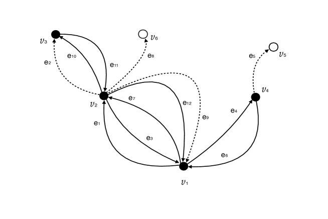
Figure 2: The tree-type diagram ${\cal D}=\hat{\cal D}$

2.3.1 Diagrams and close walks

Given a diagram ${\cal D}$, one can obtain a sequence of $k+1$ letters from the ordered alphabet ${\mathbb{U}}=\{\upsilon_{1},\upsilon_{2},\dots\}$ by starting at the root vertex $\upsilon_{1}$ and recording the vertices that appear during the chronological run over ${\cal D}$ determined by its ordered edges. We denote this sequence of letters by ${\cal W}={\cal W}({\cal D})$ and say that each edge $e_{t}$, $1\leq t\leq k$ of ${\cal D}$ represents the $t$-th step of the walk ${\cal W}$. The only convenience is that in the walk constructed we add an additional inverse step $(\upsilon^{\prime\prime},\upsilon^{\prime})$ that follows immediately after that the direct step $(\upsilon^{\prime},\upsilon^{\prime\prime})$ is performed along the red edge of ${\cal D}$. One can say that the inverse step $(\upsilon^{\prime\prime},\upsilon^{\prime})$ is the mute one and denote this couple of steps by $[\upsilon^{\prime}\upsilon^{\prime\prime}\upsilon^{\prime}]$. We consider $[\upsilon^{\prime}\upsilon^{\prime\prime}\upsilon^{\prime}]$ as one generalized step and say that the vertex $\upsilon^{\prime\prime}$ is represented in ${\cal W}$ by a generalized letter that we denote by brackets $[\upsilon^{\prime\prime}]$. Thus the total number of ordinary and generalized steps is equal to the number of edges in ${\cal D}$, $P+Q=k$ and the walk ${\cal W}$ is represented as a sequence of $k+1$ generalized letters. It is natural to say that the walk is closed and that it performs either blue step or red step when it goes along the blue edge (once) and along the red one (twice), respectively. Regarding the diagram ${\cal D}=\hat{\cal D}$ of Figure 2, we get the closed walk

$${\cal W}_{12}(\hat{\cal D})=(\upsilon_{1},\upsilon_{2},[\upsilon_{3}],\upsilon_{1},\upsilon_{4},[\upsilon_{5}],\upsilon_{1},\upsilon_{2},[\upsilon_{6}],[\upsilon_{1}],\upsilon_{3},\upsilon_{2},\upsilon_{1}).$$

Given a diagram ${\cal D}$, the walk ${\cal W}({\cal D})$ is uniquely determined. If ${\cal D}$ is a tree-type diagram, we say that ${\cal W}({\cal D})$ is a tree-type walk. We determine the set of all possible tree-type walks by equality

$$\hat{\mathbb{W}}_{k}=\left\{{\cal W}:{\cal W}({\cal D}),{\cal D}\in\hat{\mathbb{D}}_{k}\right\}.$$

We attribute to a walk ${\cal W}$ its weight determined by relation $\Pi({\cal W})=\Pi({\cal D})$, ${\cal W}={\cal W}({\cal D})$ (see (2.15)).

Inversely, one can define a closed walk ${\cal W}_{k}=(\upsilon(1),\dots,\upsilon(k+1))$ as a sequence of letters taken from the ordered alphabet ${\cal U}=\{\upsilon_{1},\upsilon_{2},\dots\}$ that starts and ends with $\upsilon_{1}$,

$$\upsilon(1)=\upsilon(k+1)=\upsilon_{1},$$

verifies condition $\upsilon(t+1)\neq\upsilon(t)$ for all $t$, $1\leq t\leq k$; we assume that ${\cal W}_{k}$ is such that at each instant of time $t+1$ the value $\upsilon(t+1)$ either belongs to the set ${\mathbb{U}}_{t}$ of already existing letters or is equal to a new letter $\upsilon_{1+\#{\mathbb{U}}_{t}}$. Some letters of the collection $\{\upsilon(t),2\leq t\leq k\}$ can be marked as the special (or generalized) ones that we put into the brackets. The remaining non-marked letters are referred to as the ordinary ones.

Regarding a walk ${\cal W}_{k}$, we can uniquely determine ${\cal D}_{k}={\cal D}({\cal W}_{k})$. To do this, we perform the chronological run along ${\cal W}_{k}$ and draw the vertices and edges between them by the rules described in sub-section 2.1 when constructing ${\cal D}$ for a realization of $k+1$ integers. If $\upsilon(t)$ is marked as the generalized letter, we find the maximal value $t-j$, $j\geq 1$ such that $\upsilon(t-j)$ is ordinary, draw one direct edge $(\upsilon(t-j),\upsilon(t))$ and return immediately to the vertex $\upsilon(t-j)$ by the mute step without drawing the inverse edge $(\upsilon(t),\upsilon(t-j))$. In the diagram obtained, we color the edges that lead to the generalized letters in red, the remaining edges are colored in blue.

If the diagram ${\cal D}({\cal W})$ is of the tree-type, we say that ${\cal W}$ is also the tree-type walk. We denote the set of all tree-type walks of $k$ steps by $\hat{\mathbb{W}}_{k}$. Now we can say that the set of all tree-type diagrams $\hat{\mathbb{D}}_{k}$ and the set of all tree-type walks $\hat{\mathbb{W}}_{k}$ are in one-to-one correspondence. The same concerns the families $\hat{\mathbb{D}}_{k}$ and $\hat{\mathbb{W}}_{k}$. Then equality

$$\sum_{{\cal D}\in\hat{\mathbb{D}}_{k}}\Pi({\cal D})=\sum_{{\cal W}\in\hat{\mathbb{W}}_{k}}\Pi({\cal W})=\Pi(\hat{\mathbb{W}}_{k})$$

together with (2.30) implies relation

$$M_{k}^{(N,R)}=\Pi(\hat{\mathbb{W}}_{k})+o(1),\ (N,R)^{\circ}\to\infty.$$

2.3.2 Total weight of tree-type walks

To describe the family of all possible tree-type walks $\hat{\mathbb{W}}_{k}$ and to compute the total weight $\Pi(\hat{\mathbb{W}}_{k})$, we develop a kind of recurrence based on the so-called first-edge decomposition procedure. The basic idea of this technique dates back to the pioneering paper [30]. In our context, we follow in major part the method developed for the tree-type walks in [17, 18].

Let us consider the root vertex $\upsilon_{1}$ of the diagram ${\cal D}({\cal W})$ and the first edge $\{\upsilon_{1},\upsilon_{2}\}$ created by the first step of any walk ${\cal W}$ of $k$ steps. If $k=0$, then $\upsilon_{2}=\upsilon_{1}$, if $k\geq 1$, then $\upsilon_{2}\neq\upsilon_{1}$. To briefly describe the essence of the first-edge recurrence method, let us consider two sub-walks of ${\cal W}$ that we denote by $\dot{\cal W}$ and $\ddot{\cal W}$. The first one produces a diagram $\dot{\cal D}$ that contains the edge $\{\upsilon_{1},\upsilon_{2}\}$ while the second one produces a diagram $\ddot{\cal D}$ that does not contain this edge. We assume that $\dot{\cal D}$ and $\ddot{\cal D}$ have no vertices in common and that the sub-walk $\dot{\cal W}$ can get to the root vertex $\upsilon_{1}$ along the edge $\{\upsilon_{1},\upsilon_{2}\}$ only. Thus by the recurrence the diagrams $\dot{\cal D}$ and $\ddot{\cal D}$ are such that their skeletons $\hat{G}(\dot{\cal D})$ and $\hat{G}(\ddot{\cal D})$ are trees. We consider all possible sub-walks $\dot{\cal W}$ and $\ddot{\cal W}$ of this kind and therefore the set of walks of $k$ steps ${\mathbb{W}}_{k}$ that we construct by this recurrence procedure contains all possible tree-type walks. This procedure also allows one to compute the total weight of walks from ${\mathbb{W}}_{k}$. Now let us give rigorous definitions to the notions used above.

We denote by ${\mathbb{W}}_{k}^{(r)}$ the family of such walks from ${\mathbb{W}}_{k}$ that have $r\geq 0$ steps either of the form $(\upsilon_{1},\upsilon_{i})$ or of the form $[\upsilon_{1}\upsilon_{i}\upsilon_{1}]$, in other words $r$ steps out of $\upsilon_{1}$ and denote by $\Theta(k,r)=\Theta^{(v,\phi_{1})}(k,r)$ the sum of the weights of all walks from ${\mathbb{W}}_{k}^{(r)}$,

$$\Theta(k,r)=\sum_{{\cal W}\in{\mathbb{W}}_{k}^{(r)}}\Pi({\cal W}).$$

If $r=0$, then ${\mathbb{W}}_{k}^{(0)}$ is non-empty if and only if $k=0$ and in this case ${\mathbb{W}}_{0}^{(0)}$ contains one trivial walk of zero steps ${\cal W}_{0}=(\upsilon_{1})$. Therefore we accept that $\Theta(k,0)=\delta_{k,0}$ for all $k\geq 0$. Let us also introduce the set of walks $\dot{\mathbb{W}}_{j}^{(g)}$ of $j$ steps such that their trees have only one edge $\{\upsilon_{1},\upsilon_{2}\}$ attached to the root $\upsilon_{1}$ and in $\dot{\cal W}_{j}^{(g)}$ there are $g$ steps either of the form $(\upsilon_{1},\upsilon_{2})$ or of the form $[\upsilon_{1}\upsilon_{2}\upsilon_{1}]$. Now we can formulate the following statement that we refer to as the first decomposition lemma [17, 18].

Lemma 2.2. For any $k\geq r\geq 1$

$$\Theta(k,r)=\sum_{g=1}^{r}\ \sum_{s=r-g}^{k-g}\ {r-1\choose g-1}\ \Upsilon(k-s,g)\,\Theta(s,r-g),\quad k\geq r\geq 1,$$

where

$$\Upsilon(k-s,g)=\sum_{{\cal W}\in\dot{\cal W}_{k-s}^{(g)}}\Pi({\cal W}).$$

Proof. Given $g\leq r$, let us consider a walk ${\cal W}$ that performs $r$ steps out of the root $\upsilon_{1}$ and $g$ steps of the form either $(\upsilon_{1},\upsilon_{2})$ or $[\upsilon_{1}\upsilon_{2}\upsilon_{1}]$. If $g=r$, then by equality $\Theta(s,0)=\delta_{s,0}$ we have $s=0$ and (2.33) takes the form $\Theta(k,r)=\Upsilon(k,r)$ that is true by the definition of $\Upsilon(k,r)$.

If $r-g>0$, then there exists at least one step of ${\cal W}$ of the form either $(\upsilon_{1},\upsilon_{i})$ or $[\upsilon_{1}\upsilon_{i}\upsilon_{1}]$ such that $\upsilon_{i}\neq\upsilon_{2}$. Denoting by $\dot{\tau}_{1}$ the instant of time of the first step of this kind, we can consider the sub-walk $\dot{\cal W}^{(1)}_{\ddot{\tau}_{1}-1}=({\cal W}(1),\dots,{\cal W}(\dot{\tau}_{1}-1))$ of $\ddot{\tau}_{1}-1$ steps. We say that $\dot{\cal W}^{(1)}_{\ddot{\tau}_{1}-1}$ is the partial sub-walk of the A-type. Regarding the run of the walk after the instant $\ddot{\tau}_{1}-1$, we find the first instant of time $\dot{\tau}_{2}>\ddot{\tau}_{1}$ such that the step $({\cal W}(\dot{\tau}_{2}-1),{\cal W}(\dot{\tau}_{2}))$ is equal to either $(\upsilon_{1},\upsilon_{2})$ or $[\upsilon_{1}\upsilon_{2}\upsilon_{1}]$. We say that the sub-walk of ${\cal W}$ given by the sequence $({\cal W}(\ddot{\tau}_{1}),\dots,{\cal W}(\dot{\tau}_{2}-1))=\ddot{\cal W}^{(1)}_{\dot{\tau_{2}}-\ddot{\tau}_{2}}$ is the partial sub-walk of the B-type. Then we proceed by construction of the partial sub-walks $\dot{\cal W}^{(l)},l\geq 2$ and $\ddot{\cal W}^{(j)},j\geq 2$, if they exist. Denoting by $s$ the total number of steps in the partial B-type sub-walks we can consider the following two new sub-walks of ${\cal W}$

$$\dot{\cal W}_{k-s}=({\cal W}(1),\dots,{\cal W}(\ddot{\tau}_{1}-1),{\cal W}(\dot{\tau}_{2}),\dots,{\cal W}(\ddot{\tau}_{2}-1),\dots)=\uplus_{l\geq 1}\dot{\cal W}^{(l)}$$

that we refer to A-type sub-walk and B-type sub-walk of ${\cal W}$, respectively. and

$$\ddot{\cal W}_{s}=\uplus_{j\geq 1}\ddot{\cal W}^{(j)},$$

where we do not indicate the number of steps in the A-type and B-type partial sub-walks in order not to complicate the denotations. By the construction, $\dot{\cal W}_{k-s}\in\check{\mathbb{W}}_{k-s}^{(g)}$ while $\ddot{\cal W}_{s}\in{\mathbb{W}}_{s}^{(r-g)}$.

Regarding the walk ${\cal W}_{12}$ (2.31), we see that the B-type sub-walk $\ddot{\cal W}_{3}$ is given by one part of three steps, $\ddot{\cal W}_{3}=(\upsilon_{1},\upsilon_{4},[\upsilon_{5}],\upsilon_{1})$. Here $\ddot{\tau}^{(1)}=4$ and $\dot{\tau}^{(2)}=7$. The A-type sub-walk of ${\cal W}_{12}$ is given by the composition of two partial sub-walks; the first one consists of three steps, $\dot{\cal W}^{(1)}=(\upsilon_{1},\upsilon_{2},[\upsilon_{3}],\upsilon_{1})$ and the second one has six steps, $\dot{\cal W}^{(2)}=(\upsilon_{1},\upsilon_{2},[\upsilon_{6}],[\upsilon_{1}],\upsilon_{3},\upsilon_{2},\upsilon_{1})$, so that

$$\dot{\cal W}_{9}=(\upsilon_{1},\upsilon_{2},[\upsilon_{3}],\upsilon_{1},\upsilon_{2},[\upsilon_{6}],[\upsilon_{1}],\upsilon_{3},\upsilon_{2},\upsilon_{1}).$$

In this example, $r=3$, $g=2$ and $s=3$.

Let us denote by ${\mathbb{W}}_{k}^{(r,g)}(s)$ the family of walks ${\cal W}_{k}$ that perform $r$ steps out from the root $\upsilon_{1}$ with $g$ steps of the form either $(\upsilon_{1},\upsilon_{2})$ or $[\upsilon_{1}\upsilon_{2}\upsilon_{1}]$, $1\leq g\leq r$ and such that its B-type sub-walk $\ddot{\cal W}_{s}$ consists of $s$ steps. By construction, ${\cal W}_{k}$ uniquely determines its A-type sub-walk $\dot{\cal W}_{k-s}$ and B-type sub-walk $\ddot{\cal W}_{s}$. However, the pair $(\dot{\cal W}_{k-s},\ddot{\cal W}_{s})$ does not determines uniquely ${\cal W}_{k}$ because when creating $\dot{\cal W}_{k-s}$ we have lost the information about the repartition of $\dot{\cal W}_{k-s}$ into the partial sub-walks $\dot{\cal W}^{(l)}$. The same is true for the B-type sub-walk $\ddot{\cal W}_{s}$. This means that to determine uniquely ${\cal W}_{k}$ by its A-type sub-walk and B-type sub-walk, we have to know an additional information about the next in turn step out from $\upsilon_{1}$ - does it belong to the A-type partial sub-walk or to the B-type partial sub-walk.

The maximally possible number of partial sub-walks of $\dot{\cal W}_{k-s}$ is given by the number of the steps out from $\upsilon_{1}$ and this is $g$. The maximally possible number of partial sub-walks of $\ddot{\cal W}_{s}$ is also equal to the number of the steps out from $\upsilon_{1}$ and this is $r-g$. The first step out from $\upsilon_{1}$ always belongs to the A-type partial sub-walk. Then we observe that there are ${r-1\choose g-1}$ possibilities to attribute $g-1$ labels ”A” to $r-1$ steps out form $\upsilon_{1}$, the remaining get the labels ”B”. Since the first and the second components of $(\dot{\cal W}_{k-s},\ddot{\cal W}_{s})$ can be independently chosen from $\dot{\mathbb{W}}_{k-s}^{(g)}$ and ${\mathbb{W}}_{s}^{(r-g)}$, respectively, we can write that

$$\#{\mathbb{W}}_{k}^{(r,g)}(s)={{r-1}\choose{g-1}}\times\#\dot{\mathbb{W}}^{(g)}_{k-s}\times\#{\mathbb{W}}^{(r-g)}_{s}.$$

Taking into account that by definition ${\cal D}(\dot{\cal W}_{k-s})$ and ${\cal D}(\ddot{\cal W}_{s})$ have no edges in common, we can write that $\Pi({\cal W}_{k})=\Pi(\dot{\cal W}_{k-s})\Pi(\ddot{\cal W}_{s})$, and therefore

$$\sum_{{\cal W}\in{\mathbb{W}}_{k}^{(r,g)}(s)}\Pi({\cal W})={r-1\choose g-1}\times\sum_{\dot{\cal W}\in\dot{\mathbb{W}}^{(g)}_{k-s}}\Pi(\dot{\cal W})\times\sum_{\ddot{\cal W}\in\in{\mathbb{W}}^{(r-g)}_{s})}\Pi{(\ddot{\cal W})}.$$

Summing both parts of (2.34) over $r$, $g$ and $s$, we get equality (2.33). Lemma 2.2 is proved. $\Box$

The second decomposition lemma concerns $\Upsilon(k-s,g)$ given by the total weight of walks from the set $\dot{\mathbb{W}}_{k-s}^{(g)}$. In what follows, $g$ represents the sum of $w\geq 0$ blue steps of the form $(\upsilon_{1},\upsilon_{2})$ and $f\geq 0$ red steps of the form $[\upsilon_{1}\upsilon_{2}\upsilon_{1}]$ performed by a walk from $\dot{\mathbb{W}}_{k-s}^{(g)}$, $g=w+f$.

Lemma 2.3. The following relation holds,

$$\Upsilon(k-s,g)=\sum_{w=0}^{g}\ \sum_{h=0}^{k-s-g}\ \ \sum_{t=0}^{k-s-g-w-h}\ {v^{2(g+h)}\over\phi_{1}^{g+h-1}}\,$$

$$\times\ {g\choose w}\ {w+h-1\choose h}^{*}\,\,{w+h+t-1\choose t}^{*}\ \,\Theta(k-s-g-w-h,t),$$

for any $g\geq 1$, $k-s\geq g$.

Proof. Among $g$ steps from $\upsilon_{1}$ to $\upsilon_{2}$, we have to point out $w$ steps that will be the blue ones. This gives the first binomial coefficient of (2.35). Since each blue step is coupled with the inverse blue step, the walk has to perform $w$ blue steps of the form $(\upsilon_{2},\upsilon_{1})$. Assuming that the walk $\dot{\cal W}_{k-s}^{(g)}$ makes $h$ red steps of the form $[\upsilon_{2}\upsilon_{1}\upsilon_{2}]$ and taking into account the fact that the last step from $\upsilon_{2}$ to $\upsilon_{1}$ is the blue one, we have to point out among $w+h-1$ steps from $\upsilon_{2}$ to $\upsilon_{1}$ $w-1$ blue steps. This gives the second binomial coefficient from the right-hand side of (2.35). Finally, assuming that the walk $\dot{\cal W}_{k-s}^{(g)}$ performs $t$ steps of the form either $(\upsilon_{2},\upsilon^{\prime})$ or $[\upsilon_{2}\upsilon^{\prime}\upsilon_{2}]$ such that $\upsilon^{\prime}\neq\upsilon_{1}$, we have to point out these $t$ steps among $w+h+t-1$ steps out from $\upsilon_{2}$ performed by the walk. This gives the last binomial coefficient from the right-hand side of (2.35).

We see that in $\dot{\cal W}_{k-s}^{(g)}$ the exists a number of partial sub-walks each of them starting and ending at $\upsilon_{2}$ that do not contain the letter $\upsilon_{1}$, either ordinary or generalized. Gathering these partial sub-walks into the one sub-walk we get an element of ${\mathbb{W}}_{k-s-g-w-h}^{(t)}$. We refer to this sub-walk as the upper sub-walk of $\dot{\cal W}_{k-s}^{(r)}$. The total weight of the elements of the set ${\mathbb{W}}_{k-s-g-w-h}^{(t)}$ is given by the factor $\Theta(k-s-g-w-h,t)$ standing in the right-hand side of (2.35).

Given $w$ and $h$, we see that the multi-edge ${\upsilon_{1},\upsilon_{2}}$ of ${\cal D}({\cal W}_{k})$, ${\cal W}_{K}\in\dot{\mathbb{W}}_{k-s}^{(g)}$ contains $2w$ blue edges and $g-w+h$ red edges. According to the definition of $\Pi({\cal W})$, this multi-edge produces the factor $v^{2(g+h)}/\phi_{1}^{g+h-1}$ in (2.35).

To show that the lower limits of summation of (2.35) are correctly indicated, let us consider the contribution of the walks with $w=0$. This means that the first edge from $\upsilon_{1}$ to $\upsilon_{2}$ of the corresponding diagram ${\cal D}$ does not contain any blue edge and therefore there are no blue edges of the form $(\upsilon_{2},\upsilon_{1})$. The walk passes the edge $(\upsilon_{1},\upsilon_{2})$ $g$ times by the red edges and the upper sub-walk is empty. Regarding the right-hand side of (2.35) and remembering property (2.5), we see that if $w=0$, then $h=0$ and $t=0$. Then equality $\Theta(k-s-g-w-h,0)=\delta_{k-s-g,0}$ implies that $k-s-g=0$ and that $\Upsilon(g,g)=v^{2g}/\phi_{1}^{g-1}$. Lemma 2.3 is proved. $\Box$

Combining (2.33) and (2.35), we get relation (2.4). It follows from the definition of $\Theta(k,r)$ and (2.3) that

$$\Pi(\hat{\mathbb{W}}_{k})=\sum_{r=1}^{k}\Theta(k,r)=m_{k}^{(v,\phi_{1})}$$

and then (2.32) implies (2.2). This completes the proof of Theorem 2.1.

2.4 Limiting transition of infinite $\phi_{1}$

Let us study $m_{k}^{(v,\phi_{1})}$ (2.3) in the limiting transition $\phi_{1}\to\infty$. Regarding (2.4), we observe that the only term that gives a non-vanishing contribution to the the right-hand side of (2.4) corresponds to the case of $g+h=1$. Since $g\geq 1$, then $h=0$ and $w$ can take only two values, zero and one. Taking into account this observation and denoting

$$\theta(k,r)=\lim_{\phi_{1}\to\infty}\Theta^{(\phi_{1})}(k,r),$$

we deduce from (2.35) relation

$$\Upsilon(k-s,1)=v^{2}\sum_{w=0,1}\sum_{t=0}^{k-s-1-w}{1\choose w}\ {w-1\choose 0}^{*}\ {w+t-1\choose t}^{*}\ \theta(k-s-1-w,t)$$

$$=v^{2}\theta(k-s-1,0)+v^{2}\sum_{t=0}^{k-s-2}\theta(k-s-2,t)=v^{2}\delta_{k-s-1,0}+v^{2}\sum_{t=0}^{k-s-2}\theta(k-s-2,t).$$

Substituting this expression into (2.33), we conclude that

$$\theta(k,r)=v^{2}\theta(k-1,r-1)+v^{2}\,\sum_{s=r-1}^{k-1}\ \theta(s,r-1)\sum_{t=0}^{k-s-2}\theta(k-s-2,t).$$

Denoting

$$\mu_{k}=\sum_{r=1}^{k}\theta(k,r)$$

and changing the order of summation in the second term of (2.36), we get the following recurrence that determines $\{\mu_{k}\}_{k\geq 0}$,

$$\mu_{k}=v^{2}\mu_{k-1}+v^{2}\sum_{j=0}^{k-2}\mu_{j}\,\mu_{k-j-2},\quad k\geq 2$$

with obvious initial values $\mu_{0}=1$ and $\mu_{1}=v^{2}$. Regarding the generating function

$$g(z)=-\sum_{k=0}^{\infty}\mu_{k}{1\over z^{k+1}},$$

one can easily deduce from (2.37) relation

$$g(z)={1\over v^{2}-z-v^{2}g(z)}.$$

Equation (2.38) is uniquely solvable in the class of functions $g(z)$ such that $\hbox{Im\,}z\cdot\hbox{Im\,}g(z)\geq 0$ and therefore $g(z)$ represents the Stieltjes transform of the limiting measure $\tilde{\sigma}(\lambda)$ that is the widely known Wigner semi-circle distribution [30] shifted by $v^{2}$;

$${d\tilde{\sigma}_{v}\over d\lambda}={1\over 2\pi v^{2}}\begin{cases}\sqrt{4v^{2}-(\lambda-v^{2})^{2}},&\text{if $|\lambda-v^{2}|\leq 2|v|$},\\ 0,&\text{otherwise.}\end{cases}$$

This eigenvalue distribution has been already obtained as the eigenvalue distribution of the random matrices of the form (1.14) determined for the Erdős-Rényi random graphs in the limit of the infinite average vertex degree, $\rho\to\infty$ [16].

To complete this section, let us note that by repeating the proof of Theorem 2.1, it is not hard to show that the moments of the normalized adjacency matrix $\tilde{A}_{N}^{(R)}$ (1.14) converge in the limit $(N,R)^{\circ}\to\infty$,

$$\lim_{(N,R)^{\circ}\to\infty}{\bf\,E}\left({1\over N}{\mathrm{\,Tr}}\left(\tilde{A}_{N}^{(R)}\right)^{k}\right)=\ell_{k}^{(v,\phi_{1})}=\begin{cases}L_{p}^{(v,\phi_{1})},&\text{if $k=2p$},\\ 0,&\text{if $k=2p+1$}\end{cases}$$

for given $k=0,1,2,\dots$, where the moments $L_{p}^{(v,\phi_{1})}=\sum_{r=1}^{p}\Lambda(p,r)$, $p\geq 0$ can be found from the following recurrent relations [17, 18],

$$\Lambda(p,r)=\sum_{g=1}^{r}\ {v^{2g}\over\phi_{1}^{g-1}}{r-1\choose g-1}\sum_{s=r-g}^{p-g}\Lambda(s,r-g)\sum_{t=0}^{p-s-g}{g+t-1\choose t}\Lambda(p-s-g,t),$$

with the initial conditions $\Lambda(p,0)=\delta_{p,0}$, $p=0,1,2,\dots$

Introducing the auxiliary numbers

$${\mathfrak{L}}^{(i)}_{p}=\sum_{r=0}^{p}\ {(r+1)(r+2)\cdots(r+i-1)\over 1\cdot 2\cdots(i-1)}\Lambda(p,r),$$

where $i=1,\dots,p,$ it is easy to deduce from (2.41) relation

$${\mathfrak{L}}^{(1)}_{p}=v^{2}\sum_{j=0}^{p-1}\ {\mathfrak{L}}^{(1)}_{p-1-j}\,{\mathfrak{L}}^{(1)}_{j}+{v^{2}\over\phi_{1}}\sum_{j=0}^{p-2}\ {\mathfrak{L}}^{(2)}_{p-2-j}\,{\mathfrak{L}}^{(2)}_{j}+\dots+{v^{2p}\over\phi_{1}^{p-1}}{\mathfrak{L}}^{(p)}_{0}{\mathfrak{L}}^{(p)}_{0}.$$

It follows from (2.42) that

$$\lim_{\phi_{1}\to\infty}{\mathfrak{L}}^{(1)}_{p}\to{\cal L}_{p}(v),$$

where ${\cal L}_{p}(v)$ verifies the famous recurrence

$${\cal L}_{p}(v)=v^{2}\ \sum_{j=0}^{p-1}\ {\cal L}_{p-1-j}(v)\,{\cal L}_{j}(v),\quad{\cal L}_{0}(v)=1$$

that determines the moments of the Wigner semi-circle distribution [30],

$${\cal L}_{p}(v)=v^{2p}{(2p)!\over p!\,(p+1)!},\quad p=0,1,2,\dots$$

Then (2.42) can be regarded as a generalization of (2.44) to the case of the random graphs with the average vertex degree $\phi_{1}$ finite.

Taking into account (2.42), we observe that the moments of $\tilde{A}_{N}^{(R)}$ (2.40) converge in the additional limiting transition $\phi_{1}\to\infty$

$$\lim_{\phi_{1}\to\infty}L^{(v,\phi_{1})}_{2p}={\cal L}_{p}(v)$$

and therefore the limiting eigenvalue distribution of $\tilde{A}_{N}^{(R)}$ weakly converges in average in the limit $(N,R)^{\circ}\to\infty$ (1.10) and $\phi_{1}\to\infty$ to the semi-circle distribution.

3 Ihara zeta function of large random graphs

Let us discuss our results in relations with the properties of Ihara zeta function and the graph theory Riemann Hypothesis. In contrast with the previous sections, some statements are non-rigorous here in the sense that they are based on relations that are not proved yet. However, the conjectures we formulate could be regarded as a source of new interesting questions of spectral theory of large random matrices.

3.1 Weak convergence of eigenvalue distribution

First of all, let us say that the limiting moments $m_{k}^{(v,\phi_{1})}$ (2.3) verify the upper bound

$$m_{k}^{(v,\phi_{1})}\leq(C_{1}v^{2})^{k}k^{k+1}$$

with a constant $C_{1}\geq C=C(v,\phi_{1})$ (see Section 4 for the proof). The Carleman’s condition (see e.g. monograph [1]) is obviously satisfied,

$$\sum_{l\geq 0}{1\over\left(m_{2l}^{(v,\phi_{1})}\right)^{1/(2l)}}=+\infty$$

and therefore the limiting measure $\sigma^{(v,\phi_{1})}$ is uniquely determined by the family $\{m_{k}^{(v,\phi_{1})}\}_{k\geq 0}$. Then we can say that Theorem 2.1 implies the weak convergence in average of measures $\sigma_{N,R}$ to $\sigma^{(v,\phi_{1})}$. This means that for any continuous bounded function $f$: ${\mathbb{R}}\mapsto{\mathbb{R}}$ the following is true,

$$\lim_{(N,R)^{\circ}\to\infty}\ \int_{{\mathbb{R}}}f(\lambda)\,d\bar{\sigma}_{N,R}(\lambda)=\int_{{\mathbb{R}}}f(\lambda)\,d\sigma^{(v,\phi_{1})}(\lambda).$$

Relation (1.13) can be rewritten as

$$\Psi_{N}^{(R)}(v)={1\over N}\log\hbox{det}\left(\left(1-{v^{2}\over\phi_{1}}\right)I+H_{N}^{(R)}(v)\right)$$

$$=\int_{{\mathbb{R}}}\log(1_{\phi_{1}}+\lambda)\,d\sigma_{N,R}(\lambda),$$

where we denoted $1_{\phi_{1}}=1-v^{2}/\phi_{1}$. By this relation, the problem of convergence of IZF for a sequence of infinitely increasing graphs can be reduced to the analysis of convergence of the spectral measures of operators $H^{(R)}_{N}$. This approach to the studies of IZF has been proposed for the first time in paper [12].

Taking into account the weak convergence of measures (3.2), one could expect that the mathematical expectation of (3.3) ${\bf\,E}\Psi_{N}^{(R)}(v/\sqrt{\phi_{1}})$, $v\in{\mathfrak{I}}$ exists for some non-zero interval ${\mathfrak{I}}\subset\mathbb{R}$ and converges in average to the integral over $d\sigma^{(v,\phi_{1})}$ (3.2),

$${\bf\,E}\Psi_{N}^{(R)}(v/\sqrt{\phi_{1}})\to\int_{{\mathbb{R}}}\log(1_{\phi_{1}}+\lambda)\,d\sigma^{(v,\phi_{1})}(\lambda),\quad{\hbox{as}}\quad(N,R)^{\circ}\to\infty$$

and then

$$\lim_{(N,R)^{\circ}\to\infty}{1\over N}{\bf\,E}\log Z_{{\Gamma}_{N}^{(R)}}(v/\sqrt{\phi}_{1})=-\left({\phi_{1}\over 2}-1\right)\log\left(1-{v^{2}\over\phi_{1}}\right)-\Psi(v/\sqrt{\phi_{1}}),$$

where we denoted

$$\Psi(v/\sqrt{\phi_{1}})=\int_{{\mathbb{R}}}\log(1+\lambda)\,d\sigma^{(v,\phi_{1})}(\lambda).$$

Although convergence (3.4) is not proved, let us note that accepting that the limiting transition $\phi_{1}\to\infty$ can be performed in (3.5) and assuming that the limiting equality holds, one could expect that

$$\lim_{\phi_{1}\to\infty}\lim_{(N,R)^{\circ}\to\infty}{1\over N}{\bf\,E}\log Z_{{\Gamma}_{N}^{(R)}}(v/\sqrt{\phi}_{1})={v^{2}\over 2}-\Upsilon(v),$$

where

$$\Upsilon(v)={1\over 2\pi v^{2}}\int_{-2|v|+v^{2}}^{2|v|+v^{2}}\log(1+\lambda)\,\sqrt{4v^{2}-(\lambda-v^{2})^{2}}d\lambda$$

and therefore one could conclude that

$$\lim_{\phi_{1}\to\infty}\lim_{(N,R)^{\circ}\to\infty}{1\over N}{\bf\,E}\log Z_{{\Gamma}_{N}^{(R)}}({v\over\sqrt{\phi}_{1}})={\cal F}(v),$$

where

$${\cal F}(v)={v^{2}\over 2}-{2\over\pi}\int_{-1}^{1}\log(1+v^{2}+2v\tau)\sqrt{1-\tau^{2}}\,d\tau.$$

It is easy to see that the last integral exists for any real $v$ and that the limiting function is continuous for all $v\in{\mathbb{R}}$.

3.2 Graph theory Riemann Hypothesis

Regarding the family of finite regular graphs with the vertex degree $q+1$ (in other terms, $(q+1)$-regular graphs), the graph theory analog of the Riemann Hypothesis can be formulated as follows [13, 28]:

$$Z_{\Gamma}(q^{-s})\ \ {\hbox{has no poles with $0<$ Re\,$s<1$ unless Re\,$s=1/2$.}}$$

It can be shown that (3.8) is equivalent to the condition for the graph ${\Gamma}$ to be the Ramanujan one [20]; more precisely, if a connected regular graph ${\Gamma}$ verifies (3.8), then [13]

$$\rho_{\Gamma}^{\prime}\leq 2\sqrt{\rho_{\Gamma}-1},$$

where

$$\rho_{\Gamma}=\max\{|\lambda|:\ \lambda\in{\hbox{Sp}}(A_{\Gamma})\}\ \ {\hbox{and }}\ \ \rho^{\prime}_{\Gamma}=\max\{|\lambda|:\ \lambda\in{\hbox{Sp}}(A_{\Gamma}),|\lambda|\neq\rho_{\Gamma}\}$$

and where we denoted by $\hbox{Sp}(A_{\Gamma})$ the ensemble of eigenvalues of the adjacency matrix $A_{\Gamma}$ of the graph ${\Gamma}$. For any $(q+1)$-regular graph $\rho_{\Gamma}=q+1$, so condition (3.9) reads as $\rho^{\prime}_{\Gamma}\leq 2\sqrt{q}$.

Numerical simulations of [22] lead to the conjecture that the proportion of regular graphs exactly satisfying the graph theory Riemann Hypothesis approaches $27\%$ as the number of vertices $N=\#V({\Gamma})$ infinitely increases. From another hand, the Alon conjecture for regular graphs proved by J. Fridman (see [9] and also [6]) says that for any positive $\varepsilon>0$

$${1\over\#{\cal G}_{N}(q+1)}\#\left\{{\Gamma}:\ {\Gamma}\in{\cal G}_{N}(q+1),\ \rho^{\prime}_{\Gamma}\geq 2\sqrt{q}+\varepsilon\right\}\to 0,\quad N\to\infty,$$

where ${\cal G}_{N}(q+1)$ is the family of all $(q+1)$-regular graphs with the set of vertices $\{1,2,\dots,N\}$. This result means that the Riemann Hypothesis (3.8) is “approximately true” for most of regular graphs of high dimension [13].

It can be shown that (3.8) is equivalent to the statement that for finite connected $(q+1)$-regular graph ${\Gamma}$ with $q\geq 2$

$$Z_{\Gamma}(u)\ {\hbox{is pole free for}}\ {1\over q}<|u|<{1\over\sqrt{q}}.$$

For the family of irregular graphs, one can formulate the weak graph theory Riemann Hypothesis saying that [13, 27]

$$Z_{\Gamma}(u)\ {\hbox{is pole free for}}\ R_{\Gamma}<|u|<{1\over\sqrt{d_{\max}-1}},$$

where $R_{\Gamma}$ is the radius of the largest circle of convergence of the Ihara zeta function $Z_{\Gamma}(u)$ and $d_{\max}=d_{\max}({\Gamma})$ is the maximum degree of ${\Gamma}$.

Let us return to the Ihara zeta function $Z_{\Gamma_{N}^{(R)}}$ of random graphs $\Gamma^{(R)}_{N}$ (1.8) and consider the conjectured limiting expression for its normalized logarithm (3.7). It follows from the classical theorems that the limiting function ${\cal F}(v)$ (3.8) is continuous for all $v\in{\mathbb{R}}$ and therefore has no real poles. Moreover, the integral expression of the right-hand side of (3.8) can be continued to a function holomorphic in any domain

$$C_{\epsilon}=\{v:\,v\in{\mathbb{C}},|v|<1-\epsilon\},\ 0<\epsilon<1.$$

From another hand, for any $v^{\prime}\in{\mathbb{C}}$ such that $|v^{\prime}|=1$ and $v^{\prime}\neq\pm 1$, there exists $\tau^{\prime}$ such that $\log(1+v^{2}+2\tau v)\sqrt{1-\tau^{2}}$ has a non-integrable singularity at this point.

Remembering pre-limiting relation $v=u\sqrt{\phi_{1}}$ (1.12), we could deduce from (3.14) that the function $\Psi(u)=\Psi(v/\sqrt{\phi_{1}})$ (3.5) has no real poles and no complex poles $u^{\prime}$ such that

$$|u^{\prime}|<{1\over\sqrt{\phi_{1}}},$$

but has the poles lying everywhere on the circle $|u|=1/\sqrt{\phi_{1}}$, $u\in\mathbb{C}$ excepting the regular points $-1/\sqrt{\phi_{1}}$ and $1/\sqrt{\phi_{1}}$.

Now we can formulate a conjecture that the normalized logarithm of the Ihara zeta function of random graphs $Z_{\Gamma_{N}^{(R)}}(u)$ determined by (1.4) with the spectral parameter renormalized by the average vertex degree, $u=v/\sqrt{\phi_{1}}$, converges in average in the limit $N\to\infty$, $R\to\infty$ and $\phi_{1}\to\infty$ (1.6) to a function ${\cal F}(v)$ (3.8),

$$-{1\over N}{\bf\,E}\log Z_{\Gamma}\left({v\over\sqrt{\phi_{1}}}\right)\to{\cal F}(v);$$

the limiting function ${\cal F}(v)$ has no poles inside the unit circle $\{v\in\mathbb{C}:|v|<1\}$. This proposition is in agreement with (3.12) with the difference that the value $d_{\max}-1$ for non-random graphs is replaced by the averaged vertex degree $d_{\hbox{\footnotesize{av}}}=\phi_{1}$ of random graphs. Therefore the statement (3.16) can be viewed as one more relaxed version of the graph theory Riemann Hypothesis for the ensemble of infinite random graphs $\{{\Gamma}_{N}^{(R)}\}$.

A conjecture similar to (3.16) can be put forward for the ensemble of Erdős-Rényi $N$-dimensional graphs with the edge probability $\rho/N$. In this case the averaged vertex degree $d_{\hbox{\footnotesize{av}}}=\phi_{1}$ in (1.14) and (3.16) is replaced by $\rho$ and the limiting transition considered is given by $N,\rho\to\infty$, $\rho=o(N)$ [16].

Finally, let us stress that convergence (3.4) and the limiting transition (3.6) for real and for complex $v$ are assumed but not proved rigorously neither in the present paper nor in [16]. These interesting questions remain open ones that would require deep studies of fine spectral properties of the random matrix ensembles, such as the asymptotic behavior of the maximal eigenvalue of large random matrices $A_{N}^{(R,\phi)}$ (1.4). In these studies, additional restrictions could be imposed; these restrictions could be related with the ratio between $N,R$ and $\phi_{1}$ for the ensemble $H_{N}^{(R)}(v)$ and between $\rho$ and $N$ for the random matrix of [16], where the value $\rho=\log N$ is shown to be critical for the asymptotic behavior of the spectral norm (see [15] for more details).

4 Appendix: Proof of the upper bound (3.1)

In this section we will show that the moments $\{m_{k}^{(v,\phi_{1})}\}$ (2.3) and $\{L_{k}^{(v,\phi_{1})}\}$ (2.40) verify the Carleman’s condition. Lemma 4.1 Let $C$ be a constant such that

$$C\geq 1\quad{\hbox{and}}\quad C{\phi_{1}}\geq 1.$$

Then for any $p\geq 1$, the following upper bound is true,

$$\max_{1\leq r\leq p}\Lambda(p,r)\leq\left(Cv^{2}\right)^{p}\,p^{2p}.$$

Proof. We prove (4.2) by recurrence. Assuming that all terms $\Lambda(i,j)$ of the right-hand side of (2.41) verify (4.2), we deduce from (2.41) that

$$\Lambda(p,r)\leq{\left(Cv^{2}\right)^{p}\over C}\sum_{g=1}^{r}\ {1\over(C\phi_{1})^{g-1}}{r-1\choose g-1}(p-g)^{2(p-g)}\sum_{s=r-g}^{p-g}\ {p-s\choose g},$$

where we have used an obvious inequality $s^{2s}(p-s-g)^{2(p-s-g)}\leq(p-g)^{2(p-g)}$ and the well-known identity

$$\sum_{l=0}^{j}{l+i-1\choose l}={i+j\choose i},\quad i\geq 1.$$

Changing variables in the last sum of (4.3), using a version of (4.4)

$$\sum_{i=0}^{p-r}{g+i\choose i}=\sum_{i=0}^{p-r}{g+i\choose g}={g+p-r+1\choose g+1},$$

and taking into account (4.1), we can write that

$$\Lambda(p,r)\leq\left(Cv^{2}\right)^{p}\sum_{g=1}^{r}{r-1\choose g-1}(p-g)^{2(p-g)}(p-r+1)^{g+1}$$

$$\leq\left(Cv^{2}\right)^{p}p^{p+1}\sum_{g=1}^{r}\ {r-1\choose g-1}(p-g)^{p-g}$$

$$\leq\left(Cv^{2}\right)^{p}p^{p+1}(p-1)^{p-r}\sum_{g^{\prime}=0}^{r-1}{r-1\choose g^{\prime}}(p-1-g^{\prime})^{r-1-g^{\prime}}\leq\left(Cv^{2}\right)^{p}p^{2p}.$$

Lemma 4.1 is proved. $\Box$

It follows from (4.2) that $L_{p}^{(v,\phi_{1})}\leq p^{2p+1}$ and the series $\sum_{p\geq 0}(L_{p}^{(v,\phi_{1})})^{-1/(2p)}$ diverges. Thus the family of moments $\left\{\ell_{k}^{(v,\phi_{1})}\right\}_{k\geq 0}$ (2.40) verifies the Carleman’s condition (see e.g. monograph [1]).

Lemma 4.2 The following upper bound

$$\max_{1\leq r\leq k}\tilde{\Theta}(k,r)\leq(Cv^{2}k)^{k},\quad k\geq 1$$

for any positive $C$ such that

$${1\over C}\left(1+{1\over Cv^{2}}\right)\exp\left\{{1\over C\phi_{1}}\right\}\leq 1\quad{{and}}\quad{1\over C\phi_{1}}\left(1+{1\over Cv^{2}}\right)\leq 1.$$

Proof. Assuming that all terms of the right-hand side of (2.4) verify (4.6), we get inequality

$$\Theta(k,r)\leq\sum_{g=1}^{r}\ \sum_{s=r-g}^{k-g}{r-1\choose g-1}\ \sum_{w=0}^{g}\ {g\choose w}\sum_{h=0}^{k-s-g-w}\ \ {v^{2(g+h)}\over\phi_{1}^{g+h-1}}$$

$$\times\ {w+h-1\choose h}^{*}\ {k-s-g\choose w+h}\ \left(Cv^{2}(k-g-w-h)\right)^{k-g-w-h},$$

where we have used an obvious generalization of (4.4),

$$\sum_{l=0}^{j}{l+i-1\choose l}^{*}={i+j\choose i},\quad i\geq 0.$$

Taking into account that $(k-g-w-h)^{k-g-w-h}\leq(k-g)^{k-g-w-h}$ and using elementary inequalities

$${k-s-g\choose w+h}\leq{(k-g)^{w+h}\over(w+h)!},\quad w\geq 0,\,h\geq 0$$

and

$${w+h-1\choose h}^{*}{1\over(w+h)!}\leq{1\over h!},\quad w\geq 0,\,h\geq 0,$$

we can write that

$$\sum_{w=0}^{g}\ {g\choose w}\sum_{h=0}^{k-s-g-w}\ \ {v^{2(g+h)}\over\phi_{1}^{g+h-1}}{w+h-1\choose h}^{*}{k-s-g\choose w+h}\ \left(Cv^{2}(k-g)\right)^{k-g-w-h}$$

$$\leq\left(Cv^{2}(k-g)\right)^{k-g}\ \sum_{w=0}^{g}{g\choose w}\sum_{h=0}^{k-s-g-w}{1\over h!}\cdot{v^{2(g+h)}\over\phi_{1}^{g+h-1}}\cdot{1\over\left(Cv^{2}\right)^{w+h}}$$

$$\leq{v^{2g}\over\phi_{1}^{g-1}}\left(Cv^{2}(k-g)\right)^{k-g\,}e^{1/(C\phi_{1})}\left(1+{1\over Cv^{2}}\right)^{g}.$$

Returning to (4.7) and replacing there the sum over $s$ by $k-g+1$, we get with the help of (4.8) the following inequalities,

$$\Theta(k,r)\leq e^{1/(C\phi_{1})}{\left(Cv^{2}\right)^{k}\over C}$$

$$\times\sum_{g=1}^{r}{r-1\choose g-1}{1\over\left(C\phi_{1}\right)^{g-1}}(k-g+1)(k-g)^{k-g}\left(1+{1\over Cv^{2}}\right)^{g}$$

$$\leq{\left(Cv^{2}\right)^{k}}e^{1/(C\phi_{1})}{1\over C}\left(1+{1\over Cv^{2}}\right)k$$

$$\times(k-1)^{k-r}\sum_{g^{\prime}=0}^{r-1}{r-1\choose g^{\prime}}(k-1)^{r-1-g^{\prime}}\left({1\over C\phi_{1}}\left(1+{1\over Cv^{2}}\right)\right)^{g^{\prime}}$$

$$\leq{\left(Cv^{2}\right)^{k}}e^{1/(C\phi_{1})}{1\over C}\left(1+{1\over Cv^{2}}\right)k^{k-r+1}\left(k-1+{1\over C\phi_{1}}\left(1+{1\over Cv^{2}}\right)\right)^{r-1}.$$

Taking into account (4.6), we get (4.5). Lemma 4.2 is proved. $\Box$

It follows from (4.5) that the upper bound (3.1) is true and therefore the family of moments $\{m_{k}^{(v,\phi_{1})}\}_{k\geq 0}$ (2.2) verifies the Carleman’s condition [1].

References

- [1] N. I. Akhiezer, The classical moment problem, Oliver & Boyd, Edinburg/London (1965) 253pp.
- [2] H. Bass, The Ihara-Selberg zeta function of a tree lattice, Internat. J. Math. 3 (1992) 717-797
- [3] M. Bauer and O. Golinelli, Random incidence matrices: moments of the spectral density, J. Statist. Phys., 103 (2001) 301-337
- [4] I. Benjamini and N. Berger, The diameter of long-range percolation clusters on finite cycles, Random Struct. Alg. 19 (2001) 102-111
- [5] B. Bollobás, Random Graphs, Cambridge studies in advanced mathematics 73, Cambridge University Press, Cambridge (2001) 498 pp.
- [6] Ch. Bordenave, A new proof of Friedman’s second eigenvalue Theorem and its extension to random lifts, Preprint arXiv:1502.04482
- [7] G. Chinta, J. Jorgenson, and A. Karlsson, Heat kernels on regular graphs and generalized Ihara zeta function formulas, Monash. Math. 178 (2015) 171-190
- [8] B. Clair and S. Mokhtari-Sharghi, Convergence of zeta function of graphs, Proc. Amer. Math. Soc. 130 (2002) 1881-1886
- [9] J. Friedman, A proof of Alon’s second eigenvalue conjecture and related problems, Mem. Amer. Math. Soc. 195: 910 (2008) viii+100
- [10] J. Friedman, Formal Zeta function expansions and the frequency of Ramanujan graphs, Preprint arXiv:1406.4557
- [11] D. Guido, T. Isola, and M.L. Lapidus, A trace on fractal graphs and the Ihara zeta function, Trans. Amer. Math. Soc. 361 (2009) 3041-3070
- [12] R. Grigorchuk and A. Zuk, The Ihara zeta function of infinite graphs, the KNS spectral measure and integrable maps, in: Random walks and geometry, Walter de Gruyter GmbH & Co. KG, Berlin, (2004) 141-180
- [13] M.D. Horton, H.M. Stark and A.A. Terras, What are zeta functions of graphs and what are they good for? In: Contemporary Mathematics Vol. 415 Quantum Graphs and Their Applications, (2006) 173-190
- [14] Y. Ihara, On discrete subgroups of the two by two projective linear group over -adic fields, J. Math. Soc. Japan 18 (1966) 219-235
- [15] O. Khorunzhiy, On high moments of strongly diluted large Wigner random matrices, Séminaire de Probabilités XLVIII, 347–399, Lecture Notes in Math., 2168, Springer (2016)
- [16] O. Khorunzhiy, On eigenvalue distribution of random matrices of Ihara zeta function of large random graphs, J. Mathem. Physics, Analysis, Geom. 13 (2017) 268-282
- [17] O. Khorunzhiy, M. Shcherbina, and V. Vengerovsky, Eigenvalue distribution of large weighted random graphs, J. Math. Phys. 45 (2004) 1648-1672
- [18] O. Khorunzhiy and V. Vengerovsky, On asymptotic solvability of random graph’s laplacians, Preprint arXiv:math-ph/0009028
- [19] D. Lenz, F. Pogorzelski and M. Schmidt, The Ihara Zeta function for infinite graphs, Preprint arXiv:1408.3522
- [20] A. Lubotzky, R. Phillips and P. Sarnak, Ramanujan graphs, Combinatorica 8 (1988) 261-277
- [21] M.L. Mehta, Random Matrices, Elsevier/Academic Press, Amsterdam ( 2004) 688 pp.
- [22] S. J. Miller and T. Novikoff, The distribution of the largest nontrivial eigenvalues in families of random regular graphs, Experiment. Math. 17 (2008) 231-244
- [23] C. E. Porter, Statistical Theories of Spectra: Fluctuations - a collection of reprints and original papers, Academic Press, New York, (1965) 576pp.
- [24] P. Ren et al., Quantum walks, Ihara zeta functions and cospectrality in regular graphs, Quantum Inf. Processes 10 (2011) 405-417
- [25] L.S. Schulman, Long range percolation in one dimension, J. Phys. A: Math. Gen. 16 (1983) L639-L641
- [26] H. M. Stark and A. A. Terras, Zeta Functions of Finite Graphs and Coverings, Adv. Math., 121 (1996) 124-165
- [27] H. M. Stark and A. A. Terras, Zeta functions of finite graphs and coverings, III, Adv. Math. 208 (2007) 467-489
- [28] A. Terras, Zeta functions and chaos, in: A Window Into Zeta and Modular Physics, MSRI Publication, Vol. 57 (2010) 145-182
- [29] A. Terras, Zeta functions of graphs, Cambridge studies in advanced mathematics, Vol. 128, Cambridge University Press, Cambridge (2011) xii+ 239pp.
- [30] E. Wigner, Characteristic vectors of bordered matrices with infinite dimensions, Ann. Math. 62 (1955) 548-564
- [31] Z.Q. Zhang, F.C. Pu and B.Z. Lin, Long-range percolation in one dimension, J. Phys. A: Math. Gen. 16 (1983) L85-L90
- [32] D. Zhou, Y. Xiao, and Y.-H. He, Seiberg duality, quiver theories, and Ihara’s zeta function, Internat. J. Modern Phys. A 30 (2015) 1550118