Phase diagram of truncated tetrahedral model

Abstract

Phase diagram of a discrete counterpart of the classical Heisenberg model, the truncated tetrahedral model, is analyzed on the square lattice, when the interaction is ferromagnetic. Each spin is represented by a unit vector that can point to one of the 12 vertices of the truncated tetrahedron, which is a continuous interpolation between the tetrahedron and the octahedron. Phase diagram of the model is determined by means of the statistical analogue of the entanglement entropy, which is numerically calculated by the corner transfer matrix renormalization group method. The obtained phase diagram consists of four different phases, which are separated by five transition lines. In the parameter region, where the octahedral anisotropy is dominant, a weak first-order phase transition is observed.

I Introduction

Symmetry breaking is one of the fundamental concepts in the field theoretical analyses. Phase transitions in statistical models are known as the typical realizations of the symmetry breaking, where the feature of transitions is dependent on symmetries in local degrees of freedom. For example, the classical Heisenberg model has the $O(3)$ symmetry, and there is ferromagnetic-paramagnetic phase transition of the second order when the model is on the cubic lattice, and when the interaction is ferromagnetic. In this case the transition temperature is of the order of the interaction energy divided by Boltzmann constant.

The $O(3)$ symmetry group has discrete subgroups, some of which correspond to polyhedral symmetries that correspond to Platonic polygons. Discrete counterpart of the classical Heisenberg model can be defined according to the polyhedral group symmetries. For example, a ferromagnetic 30-state discrete vector spin model was introduced by Rapaport, for the purpose of simplifying Monte-Carlo simulation of the three-dimensional (3D) ferromagnetic Heisenberg model Rapaport (1985). In this discretization, the middle points of the edges of the icosahedron, which has 12 vertices and 30 edges, are allowed to be the local spin degrees of freedom. It was shown that the calculated phase transition temperature coincides well with that of the 3D Heisenberg model. Margaritis et al. considered a 12-state discrete vector model, which corresponds to the icosahedral symmetry, and also the 20-state one with the dodecahedral symmetry Margaritis et al. (1987). On the cubic lattice, it was shown that the 12-state model already well represent the phase transition of the 3D Heisenberg model. Thus, in three dimensions, the effect of such discretization introduced in the 12-, 20-, and 30-state vector models is irrelevant, as long as the universality of the phase transition is concerned.

In two dimensions (2D), the situation is somewhat different. The continuous symmetry of the Heisenberg model prohibits the phase transition at finite temperature when the model is defined on 2D lattices Mermin and Wagner (1966). Thus, if a discrete symmetry is introduced, it could be a relevant perturbation. It is instructive to remind that the $q$-state clock model, the discrete analogue of the classical XY model, shows a Bereziskii-Kosterlitz-Thouless (BKT) phase transition Berezinskii (1971, 1972); Kosterlitz and Thouless (1973) when $q\geq 5$. In case of the ferromagnetic tetrahedral model on the square lattice, where only 4 states are allowed, there is a phase transition subject to the 4-state Potts universality class Wu (1982). Nienhuis et al. showed that the cubic anisotropy is relevant to the $O(3)$ symmetry on 2D lattice, and a nontrivial phase diagram was reported for the ferromagnetic case Nienhuis et al. (1983). Margaritis et al. confirmed the presence of the order-disorder phase transition in the discrete vector spin models with 12, 20, and 30 degrees of freedom on the square lattice and showed that the transition temperature is strongly dependent on the number of the local spin states Margaritis et al. (1987). Patrascioiu and Seiler performed a scaling analysis for the case of the icosahedral discretization and estimated the critical exponents assuming that the transition is of the second order Patrascioiu and Seiler (2001). A perturbative analysis of the critical behavior has been performed by Caracciolo et al., and critical indices for the tetrahedral, cubic, and octahedral cases were estimated Caracciolo et al. (2001, 2002). Surungan revisited the icosahedral and the dodecahedral cases and obtained transition temperature and critical exponents, that agree with the previous studies Surungan and Okabe (2012).

A theoretical interest in the 2D polyhedral models is being focused on cases, where the discrete symmetry group has subgroups. In such cases, successive transitions from a phase with a higher symmetry to another phase with a lower symmetry can be observed; the symmetry is only partially broken in the intermediate temperature region. Surungan et al. investigated a discrete counterpart of the Heisenberg model, the edge-cubic model, in which the local spins can point to one of the 12 vertices of the cuboctehadron Surungan et al. (2008). They detected two phase transitions; the first one in the low-temperature side of the 3-state Potts universality class, and the second one in the high-temperature side, which could be explained by the cubic symmetry. The edge-cubic model belongs to a variety of truncated Platonic — Archimedean — solid models, which can also be regarded as discrete counterparts to the classical Heisenberg model. In this work we investigate another example of the truncated models, the truncated tetrahedral model (TTM), which is defined as a continuous interpolation between the tetrahedral and the octahedral models. The reason we have chosen this case of TTM is that the octahedral case with the 6 degrees of freedom is much less studied if compared to other symmetries, and we intend to analyze the stability of the critical behavior with respect to perturbations toward the tetrahedral symmetry.

This article is organized as follows. In the next section we introduce the TTM, and briefly discuss its property around the octahedral and the tetrahedral limits. In Section III, the phase diagram in the entire parameter region is determined by means of the classical analogue of the entanglement entropy, which is calculated from the spectrum of the density matrix obtained by the Corner Transfer Matrix Renormalization Group (CTMRG) method Nishino and Okunishi (1996, 1997). We then classify the nature of the phase transition lines. The obtained results are summarized in the last section.

II Truncated Tetrahedral Model

Figure 1: The truncated tetrahedron (shown in the middle, parameterized by $t=0.5$) is depicted as the interpolation between the octahedron (on the left for $t=0$) and the tetrahedron (on the right for $t=1$).

We consider a finite-directional counterpart of the classical Heisenberg model on the 2D square lattice. Local spin on each lattice site is represented by a unit vector that can point to one of the 12 vertices of the truncated tetrahedron shown in Fig. 1, whose shape is determined by a parameter $t$ from octahedral limit $t=0$ to the tetrahedral one $t=1$. We represent the spin variable on the site that is specified by indices $i$ and $j$ by means of the unit vector $\mathbf{S}_{i,j}^{~{}}(t)$ given by

$$\mathbf{S}_{i,j}^{~{}}(t)=\sqrt{\frac{1+2t^{2}_{~{}}}{2}}\,\,\mathbf{s}^{[k]}_{~{}}(t)\,,$$ (1)

where the components of unnormalized vector $\mathbf{s}^{[k]}_{~{}}(t)$ for $k=1\sim 12$ are listed in Table 1. We assume that ferromagnetic coupling $J>0$ is present between nearest-neighbor sites, and that the interaction is represented in the form of inner product. Under these settings, the Hamiltonian of the TTM is written as

$$H_{t}^{~{}}=-J\sum_{i,\,j}^{~{}}\biggl{[}\mathbf{S}_{i,j}^{~{}}(t)\cdot\mathbf{S}_{i+1,j}^{~{}}(t)+\mathbf{S}_{i,j}^{~{}}(t)\cdot\mathbf{S}_{i,j+1}^{~{}}(t)\biggr{]}\,.$$ (2)

Table 1: The directions of the 12 vertices of the truncated tetrahedron represented by means of the unnormalized vector $\mathbf{s}^{[k]}_{~{}}(t)$.

$k$	$\mathbf{s}^{[k]}_{~{}}(t)$			$k$	$\mathbf{s}^{[k]}_{~{}}(t)$
$1$	$\Big{(}\hfill t,$	$0,$	$-\frac{1}{\sqrt{2}}\Big{)}$	$2$	$\Big{(}\hfill-t,$	$0,$	$-\frac{1}{\sqrt{2}}\Big{)}$
$3$	$\Big{(}\hfill\frac{1-t}{2},$	$\frac{1+t}{2},$	$\frac{t}{\sqrt{2}}\Big{)}$	$4$	$\Big{(}\hfill\frac{1+t}{2},$	$\frac{1-t}{2},$	$-\frac{t}{\sqrt{2}}\Big{)}$
$5$	$\Big{(}-\frac{1+t}{2},$	$\frac{1-t}{2},$	$-\frac{t}{\sqrt{2}}\Big{)}$	$6$	$\Big{(}-\frac{1-t}{2},$	$\frac{1+t}{2},$	$\frac{t}{\sqrt{2}}\Big{)}$
$7$	$\Big{(}-\frac{1-t}{2},$	$-\frac{1+t}{2},$	$\frac{t}{\sqrt{2}}\Big{)}$	$8$	$\Big{(}-\frac{1+t}{2},$	$-\frac{1-t}{2},$	$-\frac{t}{\sqrt{2}}\Big{)}$
$9$	$\Big{(}\hfill\frac{1-t}{2},$	$-\frac{1+t}{2},$	$\frac{t}{\sqrt{2}}\Big{)}$	$10$	$\Big{(}\hfill\frac{1+t}{2},$	$-\frac{1-t}{2},$	$-\frac{t}{\sqrt{2}}\Big{)}$
$11$	$\Big{(}\hfill 0,$	$t,$	$\frac{1}{\sqrt{2}}\Big{)}$	$12$	$\Big{(}\hfill 0,$	$-t,$	$\frac{1}{\sqrt{2}}\Big{)}$

As it is shown in Fig. 1, the TTM reduces to the tetrahedral model in the limit $t=1$, apart from the multiplicity of 3 for each tetrahedron vertices. One can check the equivalence $\mathbf{s}^{[1]}_{~{}}(1)=\mathbf{s}^{[4]}_{~{}}(1)=\mathbf{s}^{[10]}_{~{}}(1)$ from Table I, and the same for the groups $k=2,5,8$, $k=3,6,11$, and $k=7,9,12$. The tetrahedral model is essentially equivalent to the 4-state Potts model Wu (1982). In another limit $t=0$, the TTM reduces to the octahedral model; in this case $k=1,2$, $k=3,4$, $k=5,6$, $k=7,8$, $k=9,10$, and $k=11,12$ are the 6 direction of the octahedron vertices.

In order to obtain the phase diagram with respect to the parameter $t$ and the temperature $T$, we calculate the free energy of the TTM. Let us consider the finite size system of the size $L$ by $L$. The partition function

$$Z_{t}^{~{}}(T;L)=\sum\limits_{\{\mathbf{S}(t)\}}^{~{}}\exp\left(-\frac{H_{t}}{k_{\rm B}^{~{}}T}\right)$$ (3)

is the configuration sum of Boltzmann factor taken over all the spins denoted by $\{\mathbf{S}(t)\}$. Here, $k_{\rm B}^{~{}}$ is Boltzmann constant, and we use the dimensionless units by setting $k_{\rm B}^{~{}}=J=1$. Once $Z_{t}^{~{}}(T;L)$ is obtained for a series of system size $L$, we can estimate the free energy per site

$$f_{t}^{~{}}(T)=\lim_{L\to\infty}^{~{}}-\frac{1}{L^{2}_{~{}}}\,\,k_{\rm B}T\,\ln Z_{t}^{~{}}(T;L)$$ (4)

in the thermodynamic limit.

As a numerical tool to obtain $Z_{t}^{~{}}(T;L)$, we use the CTMRG method, which was developed from Baxter’s corner transfer matrix (CTM) formalism Baxter (1982). The method enables to calculate the partition function in the form

$$Z_{t}^{~{}}(T;L)={\rm Tr}\ C_{~{}}^{4}\,,$$ (5)

where $C$ is the CTM, which corresponds to a quadrant of the finite system Nishino and Okunishi (1996, 1997). It is convenient to define the normalized density matrix

$$\rho(T;L)=\frac{C^{4}_{~{}}}{{\rm Tr}\ C_{~{}}^{4}}=\frac{C^{4}_{~{}}}{Z_{t}^{~{}}}\,,$$ (6)

and the mean value of a local operator $O$ at the center of the system is given by $\langle O\rangle={\rm Tr}(O\rho)$. In the CTMRG calculations, we keep $m=300$ representative states at most. Further details of the free energy analysis by CTMRG can be found in Ref. Genzor et al., 2015.

A 2D classical system is related to a 1D quantum systems via so called the quantum- classical correspondence, which is justified via the path integral formulation; Fradkin and Susskind (1978) on the discrete lattice, the Suzuki-Trotter decomposition provides an explicit mapping Trotter (1958); Suzuki (1966, 1976). This correspondence enables us to introduce the notions of quantum information, such as the concurrence Osterloh et al. (2002); Osborne and Nielsen (2002) and the entanglement entropy Osborne and Nielsen (2002); Vidal et al. (2003); Franchini et al. (2007) to 2D classical systems. Let us regard the horizontal direction of our 2D classical lattice model as the space direction, and vertical direction as the imaginary time one. The lower-half lattice is then identified with the past, and the upper half is the future. In the CTM formalism, both of these halves are represented as the product $C^{2}_{~{}}$ of two CTMs, and therefore the density matrix $\rho(T;L)$ in Eq. (6) corresponds to square geometry on the 2D lattice, where there is a cut from the center of the system toward either left or right boundary with open boundary condition. The detail of this correspondence is reported by Tagliacozzo et al. Tagliacozzo et al. (2008).

Based on the quantum-classical correspondence, the classical analogue of the entanglement entropy in the current study is represented as

$$S_{v}^{~{}}(T;L)=-{\rm Tr}\ \rho\ln\rho\,\,\sim\,\,-\sum\limits_{k=1}^{m}\lambda_{k}^{~{}}\ln\lambda_{k}^{~{}}\,,$$ (7)

where $\lambda_{k}^{~{}}$ are the eigenvalues of the density matrix $\rho(T;L)$ in Eq. (6). As a consequence of the conformal invariance at criticality Belavin et al. (1984), it is known that close to a critical point, the entanglement entropy scales as $S_{v}^{~{}}(T;\infty)\sim\frac{c}{6}\,\ln\,\xi$, where $c$ is a central charge and $\xi$ is the correlation length in both 1D-quantum and 2D classical systems Holzhey et al. (1994); Korepin (2004); Calabrese and Cardy (2004); Ercolessi et al. (2010); note that we are effectively considering a system with open boundary condition. Thus $S_{v}^{~{}}(T;\infty)$ is divergent at the critical point, and can be used for finding the location of phase boundaries Tagliacozzo et al. (2008). In the case of first-order phase transition, $S_{v}^{~{}}(T;\infty)$ is discontinuous at the transition point. As examples, we show $S_{v}^{~{}}(T;L)$ when $L=1000$ for the cases $t=0.2$, $0.3$, and $0.4$ with respect to temperature $T$ in Fig. 2. It should be noted that there is no need to observe thermodynamic functions and order parameters for the determination of the phase boundary.

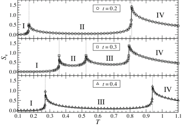
Figure 2: The temperature dependence of the classical analogue of the entanglement entropy $S_{v}^{~{}}$ for $t=0.2$, $t=0.3$, and $t=0.4$. The vertical dotted lines denote phase boundaries, and each phase is labeled by the Roman number.

III Phase Diagram

Figure 3 shows the phase diagram of the TTM determined from the singular or discontinuous behavior in $S_{v}^{~{}}$ as shown in Fig. 2. There are 4 phases, which are labeled from I to IV in the diagram. In the low-temperature side, there is a ferromagnetic phase I, where the symmetry is totally broken. The intermediate phase II in the octahedral side has the $Z_{2}^{~{}}$ symmetry, and if the directions $k=1$ and $k=2$ according to Table I are spontaneously chosen, these two directions appear equally. The intermediate phase III in the tetrahedral side has the $D_{3}^{~{}}$ symmetry, and if the directions $k=1$, $k=4$, and $k=10$ are spontaneously chosen, these three directions appear equally. The phase IV in the high temperature side is completely disordered. The phase boundaries shown by the circles are of the second-order phase transition, and those shown by the triangles are identified as first-order ones. We observe the detail of each phase boundary in the following.

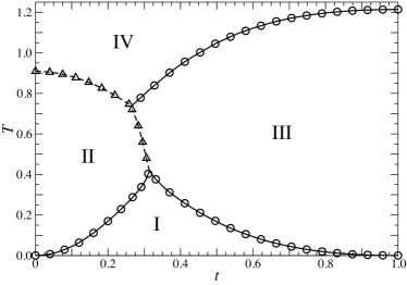
Figure 3: Phase diagram of the TTM with respect to the parameter $t$ and the temperature $T$. The circles denote the 2^nd order phase transition. The phase boundaries shown by triangles are identified as the 1^st order ones.

Let us observe the phase boundary between the phases I and II, and also the boundary between the phases I and III. When the transition is of the second order, its universality can be determined by means of finite-size corrections in thermodynamic functions Burkhardt and van Leeuwen (1982); Nishino et al. (1996). We consider the internal energy per site

$$u_{t}^{~{}}(T;L)=\frac{T^{2}_{~{}}}{L^{2}_{~{}}}\,\frac{\partial}{\partial T}\left\{k_{\rm B}^{~{}}\ln Z_{t}^{~{}}(T;L)\right\}$$ (8)

as an example. At the critical temperature $T_{\rm c}^{~{}}$, the internal energy per site satisfies

$$u_{t}^{~{}}(T_{\rm c}^{~{}};L)-u_{t}^{~{}}(T_{\rm c}^{~{}};\infty)\,\equiv\,\Delta u_{t}^{~{}}(L)\,\propto\,L^{1/\nu-2}_{~{}}\,,$$ (9)

where $\nu$ is the scaling exponent for the correlation length. One can obtain $\nu$ observing the $L$-dependence of the effective value

$$\nu_{\rm eff}(L)=\left[2+\frac{\partial\ln\Delta u_{t}^{~{}}(L)}{\partial\ln L}\right]^{-1}_{~{}}\,,$$ (10)

which is shown in Fig. 4. The results agree with the Ising universality with $\nu=1$ for the I–II phase boundary ($t=0.1$), and the 3-state Potts universality with $\nu=5/6$ for the I–III boundary ($t=0.35$).

Figure 4: The effective exponent $\nu_{\rm eff}^{~{}}(L)$ in Eq. (10) calculated at the I–II phase boundary when $t=0.1$ (squares), and that at the I–III boundary when $t=0.35$ (circles).

Figure 5: The effective exponent $\eta_{\rm eff}^{~{}}(L)$ in Eq. (12) calculated at the I–II phase boundary when $t=0.1$ (squares), and that at the I–III boundary when $t=0.35$ (circles).

In order to obtain another scaling exponent, we observe an appropriate order parameter $O_{t}^{~{}}(T;L)$, for which the finite-size correction satisfies the relation

$$O_{t}^{~{}}(T_{\rm c}^{~{}};L)\,\equiv\,\Delta O_{t}^{~{}}(L)\,\propto\,L^{-\eta/2}_{~{}}$$ (11)

noticing that $O_{t}^{~{}}(T_{\rm c}^{~{}};\infty)$ is zero. In the same manner as we have considered in Eq. (10), we can obtain $\eta$ from the effective value

$$\eta_{\rm eff}^{~{}}(L)=-2\,\frac{\partial\ln\Delta O_{t}^{~{}}(L)}{\partial\ln L}\,.$$ (12)

Inside the phase II we choose the order parameter

$$\begin{split}O_{t}^{~{}}(L)=&p_{1}+p_{2}+p_{3}+p_{4}-2p_{5}-2p_{6}+\\ &p_{7}+p_{8}-2p_{9}-2p_{10}+p_{11}+p_{12}\,.\end{split}$$ (13)

where $p_{k}^{~{}}$ are the probability of the spin at the center of the system to point to $k$-th direction listed in Table I. Inside the phase III we choose

$$\begin{split}O_{t}^{~{}}(L)=&p_{1}-p_{2}+p_{3}-p_{4}+p_{5}-p_{6}+\\ &p_{7}-p_{8}+p_{9}-p_{10}+p_{11}-p_{12}\,.\end{split}$$ (14)

Figure 5 shows the system size dependence of $\eta_{\rm eff}(L)$. The behavior at the I–II phase boundary ($t=0.1$) agrees with Ising universality class with $\eta=1/4$. At the I–III boundary, the convergence with respect to $L$ is rather slow, but $\eta_{\rm eff}(L)$ certainly approaches to the value $\eta=4/15$ of the 3-state Potts universality class.

We next observe the II–III phase boundary in the intermediate temperature region. Figure 6 shows the crossing behavior in the free energy per site $f_{t}^{~{}}(T)$ at $T=0.5$ with respect to $t$, where the crossing point is $t=0.303279$. We have chosen both fixed and free boundary conditions to weakly favor one of the two phases. Since the $Z_{2}^{~{}}$ symmetry in the phase II and $D_{3}^{~{}}$ symmetry in the phase III are not a sub-group with each other, a direct second-order phase transition between these phases is prohibited. It should be noted that the II–III boundary is not vertical in Fig. 3.

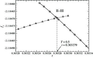
Figure 6: The free energy per site $f_{t}^{~{}}(T)$ with respect to the parameter $t$ at fixed temperature $T=0.5$ under the fixed (triangles) and the free (circles) boundary conditions.

Figure 7 shows the calculated free energy per site $f_{t=0}^{~{}}(T)$ at the octahedral limit $t=0$, which are calculated under the fixed and the free boundary conditions. Within the shown temperature region, the lower plots are thermodynamically stable, and the upper ones are quasi-stable. These two lines crosses at $T_{0}^{~{}}=0.908413$. This crossing behavior in $f_{t=0}^{~{}}(T)$ shows that the transition is of the first-order. At the transition temperature $T_{0}^{~{}}$, the internal energy per site $u_{t}^{~{}}(T;L)$ in Eq. (8) is discontinuous in the thermodynamic limit. From the jump in $u_{t}^{~{}}(T;L)$ when $L$ is sufficiently large, we obtain the latent heat $Q=0.073$. Figure 8 shows $f_{t=0}^{~{}}(T)$ when $t=0.2$. Again we observe the crossing behavior in $f_{t}^{~{}}(T)$, where the lines crosses at $T_{0}^{~{}}=0.808574$. The latent heat is estimated as $Q=0.028$. These results support the presence of a weak first-order phase transition along the II–IV phase boundary.

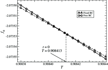
Figure 7: Temperature dependence of the free energy per site $f_{t}^{~{}}(T)$ in Eq. (4) when $t=0$, where the TTM coincides with the octahedral model. The triangles and the circles correspond to $f_{t}^{~{}}(T)$ calculated under fixed and free boundary condition, respectively.

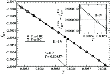
Figure 8: The free energy per site $f_{t=0.2}^{~{}}(T)$ around the II–IV phase boundary calculated for both fixed and free boundary conditions; the inset show their difference.

Since the TTM coincides with the tetrahedral model in the limit $t=1$, the critical temperature $T_{\rm c}^{~{}}$ in this limit can be calculated exactly as $T_{\rm c}^{~{}}=4J/(3\ln 3)\approx 1.21365\,J$, and the transition belongs to the 4-state Potts universality class. In this case, numerical confirmation is not straight forward, because of the nature of BKT transition Berezinskii (1971, 1972); Kosterlitz and Thouless (1973). Along the III–IV phase boundary, we observed a very slow convergence in free energy with respect to the system size $L$, which suggests the presence of BKT transition in the whole part of the III–IV boundary. We leave the confirmation of this conjecture for a future study.

IV Discussion and Conclusions

We have investigated the phase diagram and the thermodynamic properties of the truncated tetrahedral model by means of the CTMRG method. It is shown that the classical analogue of the entanglement entropy, which can be calculated from the eigenvalue spectrum of the corner transfer matrix, is efficient for the detection of the phase boundaries. Since the free energy per site is directly obtained by the CTMRG method, first-order phase transition can be directly detected as a crossing of the value.

As a result of the numerical calculation, four phases are detected. There is the ferromagnetic “phase I” in the low temperature side. In the intermediate temperature region, there are the “phase II” with $Z_{2}^{~{}}$ symmetry and the “phase III” with $D_{3}^{~{}}$ one; the boundary between these intermediate phases is of the first order. The phase transition between the completely disordered high-temperature phase, the “phase IV”, to the phase II is of the first order, where the calculated latent heat is very small. Thus in both octahedral and tetrahedral limits, the effect of the truncation is perturbative in the sense that phase II and III occupy finite area in the phase diagram, and that the phase I and IV do not touch directly. The BKT transition between the phase III and IV could be further analyzed by means of modern finite size scaling method by Hsieh et al. Hsieh et al. (2013)

The presence of the weak first-order transition on the II-IV phase boundary including the octahedral limit $t\rightarrow 0$ draws an attention to revisit both the icosahedral and the dodecahedral models, which have larger local degrees of freedom than the truncated tetrahedron model we have considered. It should be noted that the two-dimensional $q$-state Potts model show first-order phase transition when $q\geq 5$; similar first-order nature could be expected also in polyhedron models, when the site degrees of freedom is relatively large. To perform the numerical CTMRG calculation in a stable manner under icosahedral or dodecahedral symmetry is a kind of computational challenge, since the requirements on the computational memory are huge compared with the currently available computational resources.