Boolean functions whose Fourier transform is concentrated on pairwise disjoint subsets of the input

Abstract

We consider Boolean functions $f\colon\left\{\pm 1\right\}^{m}\rightarrow\left\{\pm 1\right\}$ that are close to a sum of independent functions $\left\{f_{j}\right\}$ on mutually exclusive subsets of the variables $\left\{I_{j}\right\}\subseteq P\left(\left[m\right]\right)$. We prove that any such function is close to just a single function $f_{k}$ on a single subset $I_{k}$.

We also consider Boolean functions $f\colon\mathbb{R}^{n}\rightarrow\left\{\pm 1\right\}$ that are close, with respect to any product distribution over $\mathbb{R}^{n}$, to a sum of their variables. We prove that any such function is close to one of the variables.

Both our results are independent of the number of variables, but depend on the variance of $f$. I.e., if $f$ is $\left(\epsilon\cdot{\mathrm{Var}}f\right)$-close to a sum of independent functions or random variables, then it is $O\left(\epsilon\right)$-close to one of the independent functions or random variables, respectively. We prove that this dependence on ${\mathrm{Var}}f$ is tight.

Our results are a generalization of [15], who proved a similar statement for functions $f\colon\left\{\pm 1\right\}^{n}\rightarrow\left\{\pm 1\right\}$ that are close to a linear combination of uniformly distributed Boolean variables.

1 Introduction

Perhaps the simplest characteristic of functions is linearity , i.e. functions which are simply (weighted) sums of their variables. The set of linear Boolean functions is rather limited: the only linear Boolean functions are constant functions and dictatorships, i.e. functions that depend on only one variable.

Relaxing the notion of linearity, we say that a Boolean function $f\colon\left\{\pm 1\right\}^{n}\rightarrow\left\{\pm 1\right\}$ is approximately linear if it can be approximated by an affine function of its variables, i.e. $f\approx\sum a_{i}x_{i}+a_{0}$. Another, equivalent formulation of approximately linear asserts that $f$’s Fourier coefficients are concentrated on the $1$-st and $0$-th levels, i.e. $f^{>2}\approx 0$. For example, from the latter definition it is not hard to see that such functions in particular have low noise sensitivity. Informally, low noise sensitivity means that adding a small random perturbation to the input $x$, is unlikely to change the value of $f\left(x\right)$.

A theorem of Friedgut, Kalai, Naor proves that those approximately linear functions have a unique structure: they are approximated by dictatorships.

Theorem.

(FKN Theorem, Informal [15]) Every balanced Boolean function that is almost linear is almost a dictatorship.

Intuitively, one may expect such results to be true, because a linear combination that is “well-spread” among many independent variables (i.e. far from dictatorship of one variable) should be distributed similarly to a “bell-curved” Gaussian; in particular, it should be far from the $\pm 1$ distribution of a Boolean function which is bimodal, i.e. has two distinct modes or “peaks” at $-1$ and $+1$.

1.1 The long code and related works

One of the most important historical driving forces in the study of Boolean functions has been their applications to testing of error correcting codes [6]. In particular, the long code [4] can be viewed as evaluations of dictatorships functions. Each codeword in the long code corresponds to the evaluation of a dictatorship $f\left(X\right)=x_{i}$ on all the points on the $n$-dimensional Boolean hypercube. Indeed, the long code is highly inefficient - since there are only $n$ possible dictatorships, the long code encodes $\log n$ bits of information in a $2^{n}$-bit codeword. Despite its low rate, the long code is an important tool in many results on hardness of approximation and probabilistically checkable proofs (such as [4, 18, 17, 24, 9, 23, 8, 7, 22, 2]).

The great virtue of the long code is that it is a locally testable code: It is possible to distinguish, with high probability, between a legal codeword and a string that is far from any legal codeword, by querying just a few random bits of the string. Naturally, this is a highly desirable property when constructing probabilistically checkable proofs, which are proofs that must be verified by reading a few random bits of the proof. Using local queries, it is possible to estimate whether a Boolean function is approximately linear. These properties can be used by long-code testers [8] together with the FKN Theorem described above.

1.2 Our results

In this work extend the intuition from the FKN Theorem, that a well-spread sum of independent variables must be far from Boolean. In particular we ask the following questions:

1. What happens when the variables are not uniformly distributed over $\left\{\pm 1\right\}$? In particular, we consider variables which are not even Boolean or symmetric.

   In a social choice setting, it may be intuitive to consider a mechanism that takes into account how strong is each voter’s preference. For example, in some countries the elections are known to be highly influenced by the donations the candidates manage to collect (“argentocracy”).

   In the context of computational complexity, Boolean analysis theorems that consider non-uniform distributions have proven very useful. In particular, Dinur and Safra use the $p$-biased long code in their proof of NP-hardness of approximation of the Vertex Cover problem [9]. In the $p$-biased long code each codeword corresponds to a dictatorship, in a population where each voter independently chooses $-1$ with probability $0<p<\frac{1}{2}$ and $+1$ with probability $1-p$. An extension of Friedgut’s Junta Lemma [13] to such non-uniform product distributions was key to Dinur and Safra’s proof.

   In this work we prove that even when the variables are not uniformly distributed over $\left\{\pm 1\right\}$, every Boolean function that is close to their sum must be close to one of them:

   Theorem.

   (Theorem 4.1 for balanced functions, Informal) Every balanced Boolean function that is almost a linear combination of independent functions (not necessarily Boolean or symmetric) is almost a dictatorship.

2. What happens when rather than a sum of variables, we have a sum of functions over disjoint subsets of Boolean variables?

   In a social choice setting, it may be intuitive to consider a situation where the population is divided into tribes; each tribe has an arbitrarily complex internal mechanism, but the outcomes of all the tribes must be aggregated into one communal decision by a simple (i.e. almost linear) mechanism.

   Furthermore, this theorem may lead to interesting applications in computational theory settings where such special structures arise. In fact, this was our original motivation for this work.

   Observe that this question is tightly related to the previous question because each arbitrary function over a subset of Boolean variables can be viewed as an arbitrarily-distributed random variable.

   In this work we prove that any balanced function that is close to a sum of functions over disjoint subsets of its variables is almost completely determined by a function on a single subset:

   Theorem.

   (Corollary 4.1 for balanced functions, Informal) Every balanced Boolean function that is close to a sum of functions on mutually exclusive subsets of the variables is close to a dictatorship by one subset of the variables.

As we will see later, the precise statement of the FKN Theorem does not require the Boolean function to be balanced. If we do not require the function to be balanced, there is an obvious exception to the theorem - constant functions, $f\left(X\right)=1$ and $f\left(X\right)=-1$, are not dictatorships but are considered linear. The general statement of the FKN Theorem says that a Boolean function that is almost linear is either almost a dictatorship or almost a constant function. More precisely, it says that the distance of any Boolean function from the nearest linear (not necessarily Boolean) function is smaller by at most a constant multiplicative factor than the distance from either a dictatorship or a constant function.

One may hope to extend this relaxation to non-Boolean random variables or subsets of Boolean random variables. E.g. we would like to claim that the distance of any Boolean function from a sum of functions on mutually exclusive subsets of the variables is at most the distance from a function on a single subset or a constant function. However, it turns out that this is not the case - in Lemma 4.1 we show that this naive extension of the FKN Theorem is false!

The variance of a Boolean function measures how far it is from a constant (either $-1$ or $1$). For example, the variance of any balanced Boolean function is $1$, whereas any constant function has a variance of $0$. In order to extend our results to non-balanced Boolean functions, we have to correct for the low variance. In Theorem 4.1 and Corollary 4.1 we prove that the above two theorems extend to non-balanced functions relatively to the variance:

Theorem.

(Theorem 4.1, Informal) Every Boolean-valued function that is $(\epsilon\cdot\mbox{variance})$-close to a linear combination of independent random variables (not necessarily Boolean or symmetric) is $\epsilon$-close to a dictatorship.

Theorem.

(Corollary 4.1, Informal) Every Boolean function that is $(\epsilon\cdot\mbox{variance})$-close to a sum of functions on mutually exclusive subsets of the variables is $\epsilon$-close to a dictatorship by one subset of the variables.

Intuitively these amendments to our main theorems mean that in order to prove that a Boolean function is close to a dictatorship, we must show that it is very close to linear.

Finally, in Lemma 4.1 we show that this dependence on the variance is necessary and tight.

1.3 Hypercontractivity

Many theorems about Boolean functions rely on hypercontractivity theorems such as the Bonami-Beckner Inequality ([5, 3]). Writing a real-valued function over $\left\{\pm 1\right\}^{n}$ as a polynomial yields a distribution over the monomials’ degrees $\left\{0,\dots n\right\}$, where the weight of $k$ is the sum of relative weights of monomials of degree $k$. Hypercontractivity inequalities bound the ratios between norms of real-valued functions over $\left\{\pm 1\right\}^{n}$ in terms of this distribution of weights over their monomials’ degrees. In this work it is not clear how to use such inequalities because the functions in question may have an arbitrary weight on high degrees within each subset.

All of the proofs presented in this work are completely self-contained and based on elementary methods. In particular, we do not use any hypercontractivity theorem. This simplicity makes our work more accessible and intuitive. This trend is exhibited by some recent related works, e.g. [29, 19, 25], that also present proofs that do not use hypercontractivity.

1.4 Organization

We begin with some preliminaries in Section 2. In Section 3 we give a brief survey of related works. In Section 4 we formally state our results. In Section 5 we give an intuitive sketch of the proof strategy. The interesting ingredients of the proof appear in Section 6, whereas some of the more tedious case analyses are postponed to Section 7. Tightness for some of the results is shown in Section 8. Finally, in Section 9 we make some concluding comments and discuss possible extensions.

2 Preliminaries

2.1 $L^{2}$-squared semi-metric

Throughout the paper, we define “closeness” of random variables using the squared $L^{2}$-norm:

$$\left\|X-Y\right\|_{2}^{2}={\mathrm{E}}\left[\left(X-Y\right)^{2}\right].$$

It is important to note that this is a semi-metric as it does not satisfy the triangle inequality. Instead, we will use the $2$-relaxed triangle inequality:

Fact 2.1.

$$\left\|X-Y\right\|_{2}^{2}+\left\|Y-Z\right\|_{2}^{2}\geq\frac{1}{2}\left\|X-Z\right\|_{2}^{2}.$$

Proof.

$$\left\|X-Y\right\|_{2}^{2}+\left\|Y-Z\right\|_{2}^{2}\geq\frac{1}{2}\left(\left\|X-Y\right\|_{2}+\left\|Y-Z\right\|_{2}\right)^{2}\geq\frac{1}{2}\left\|X-Z\right\|_{2}^{2}.$$

∎

Although it is not a metric, the squared $L^{2}$-norm has some advantages when analyzing Boolean functions. In particular, when comparing two Boolean functions, the squared $L^{2}$-norm does satisfy the triangle inequality because it is simply four times the Hamming distance, and also twice the $L^{1}$-norm (“Manhattan distance”): $\left\|f-g\right\|_{2}^{2}=4\cdot\Pr\left[f\neq g\right]=2\left\|f-g\right\|_{1}$.

Additionally, the squared $L^{2}$-norm behaves “nicely” with respect to the Fourier transform:

Fact 2.2.

$$\left\|f-g\right\|_{2}^{2}=\sum\left(\widehat{f}\left(S\right)-\widehat{g}\left(S\right)\right)^{2}.$$

(Proofs of Facts 2.2-2.6 are standard and are included in the appendix for completeness.)

2.2 Variance

The variance of random variable $X$ is defined as

$${\mathrm{Var}}X={\mathrm{E}}\left[X^{2}\right]-\left({\mathrm{E}}X\right)^{2}.$$

Observe that for a function $f$ the variance can also be defined in terms of its Fourier coefficients,

Fact 2.3.

$${\mathrm{Var}}f=\sum_{S\neq\emptyset}\widehat{f}\left(S\right)^{2}.$$

Another useful way to define the variance is the expected squared distance between two random evaluations:

Fact 2.4.

For any random variable X,

$${\mathrm{Var}}X=\frac{1}{2}\cdot{\mathrm{E}}_{x_{1},x_{2}\sim X\times X}\left(x_{1}-x_{2}\right)^{2}.$$

We can also view the variance as the $L^{2}$-squared semidistance from the expectation

Fact 2.5.

$${\mathrm{Var}}X=\left\|X-{\mathrm{E}}X\right\|_{2}^{2}.$$

Recall also that the expectation ${\mathrm{E}}X$ minimizes this semi-distance $\left\|X-{\mathrm{E}}X\right\|_{2}^{2}$:

Fact 2.6.

$${\mathrm{Var}}X=\min_{E\in\mathbb{R}}\left\|X-E\right\|_{2}^{2}.$$

Finally, for any two functions $f,g$ that are closed in $L^{2}$-squared semimetric, we can use the $2$-relaxed triangle inequality (Fact 2.1) to bound the difference in variance:

Fact 2.7.

$${\mathrm{Var}}f\geq\frac{1}{2}{\mathrm{Var}}g-\left\|f-g\right\|_{2}^{2}.$$

Proof.

$${\mathrm{Var}}f+\left\|f-g\right\|_{2}^{2}=\left\|f-{\mathrm{E}}f\right\|_{2}^{2}+\left\|f-g\right\|_{2}^{2}\geq\frac{1}{2}\left\|g-{\mathrm{E}}f\right\|_{2}^{2}\geq\frac{1}{2}\left\|g-{\mathrm{E}}g\right\|_{2}^{2}.$$

∎

3 Related Work

In their seminal paper [15], Friedgut, Kalai, and Naor prove that if a Boolean function is $\epsilon$-close to linear, then it must be $\left(K\cdot\epsilon\right)$-close to a dictatorship or a constant function.

Theorem.

(FKN Theorem [15]) Let $f\colon\left\{\pm 1\right\}^{n}\rightarrow\left\{\pm 1\right\}$ be a Boolean function, and suppose that $f$’s Fourier transform is concentrated on the first two levels:

$$\sum_{\left|S\right|\leq 1}\hat{f}{}^{2}\left(S\right)\geq 1-\epsilon.$$

Then for some universal constant $K$:

1. either $f$ is $\left(K\cdot\epsilon\right)$-close to a constant function; i.e. for some $\sigma\in\left\{\pm 1\right\}$

   $$\left\|f-\sigma\right\|_{2}^{2}\leq K\cdot\epsilon;$$

2. or $f$ is $\left(K\cdot\epsilon\right)$-close to a dictatorship; i.e. there exists $k\in\left[n\right]$ and $\sigma\in\left\{\pm 1\right\}$ such that $f$:

   $$\left\|f-\sigma\cdot x_{k}\right\|_{2}^{2}\leq K\cdot\epsilon.$$

   $\square$

The FKN Theorem quickly found applications in social choice theory [21]. More importantly, it has since been applied in other fields; a good example is Dinur’s combinatorial proof of the PCP theorem [8].

There are also many works on generalizations on the FKN Theorem. Alon et al. [1] and Ghandehari and Hatami [16] prove generalizations for functions with domain $\mathbb{Z}_{r}^{n}$ for $r\geq 2$. Friedgut [14] proves a similar theorem that also holds for Boolean functions of higher degrees and over non-uniform distributions; however, this theorem requires bounds on the expectation of the Boolean function. In [26], Montanaro and Osborne prove quantum variants of the FKN Theorem for any “quantum Boolean functions”, i.e. any unitary operator $f$ such that $f^{2}$ is the identity operator. Falik and Friedgut [12] and Ellis et al. [11, 10] prove representation-theory variants of the FKN Theorem, for functions which are close to a linear combination of an irreducible representation of elements of the symmetric group.

The FKN Theorem is an easy corollary once the following proposition is proven: If the absolute value of the linear combination of Boolean variables has a small variance, then it must be concentrated on a single variable. Formally,

propositionosition.

(FKN Proposition [15]) Let $\left(X_{i}\right)_{i=1}^{n}$ be a sequence of independent symmetric variables with supports $\left\{\pm a_{i}\right\}$ such that $\sum a_{i}^{2}=1$. For some universal constant $K$, if

$${\mathrm{Var}}\left|\sum_{i}X_{i}\right|\leq\epsilon,$$

then for some $k\in\left[n\right]$

$$a_{k}>1-K\cdot\epsilon.$$

$\square$

Intuitively, this proposition says that if the variance was spread among many of the variables, i.e. the “weights” $\left(a_{i}\right)$ were somewhat evenly distributed, then one would expect the sum of such independent variables to be closer to a Gaussian rather than a bimodal distribution around $\pm 1$.

This proposition has been generalized in several ways in a sequence of recent works by Wojtaszczyk [29] and Jendrej, Oleszkiewicz, and Wojtaszczyk [19], which are of particular interest to us. Jendrej et al. prove extensions of the FKN Proposition to the following cases:

1. The case where $X_{i}$’s are independent symmetric

   Theorem.

   ([19]) Let $\left(X_{i}\right)_{i=1}^{n}$ be a sequence of independent symmetric variables. Then there exists an universal constant $K$, such that for some $k\in\left[n\right]$

   $$\inf_{E\in\mathbb{R}}{\mathrm{Var}}\left|\sum_{i}X_{i}+E\right|\geq\frac{{\mathrm{Var}}\sum_{i\neq k}X_{i}}{K}.$$

   $\square$

2. The case where all the $X_{i}$’s are identically distributed

   Theorem.

   ([19]) Let $\left(X_{i}\right)_{i=1}^{n}$ be a sequence of i.i.d. variables which are not constant a.s.. Then there exists a $K_{X}$, which depends only on the distribution from which the $X_{i}$’s are drawn, such that for any sequence of real numbers $\left(a_{i}\right)_{i=1}^{n}$, for some $k\in\left[n\right]$

   $$\inf_{E\in\mathbb{R}}{\mathrm{Var}}\left|E+\sum_{i}a_{i}X_{i}\right|\geq\frac{\sum_{i\neq k}a_{i}^{2}}{K_{X}}.$$

   $\square$

Concurrent Progress by Jendrej, Oleszkiewicz, and Wojtaszczyk

Let us note that the works of Wojtaszczyk [29] and Jendrej, Oleszkiewicz, and Wojtaszczyk [19] have been eventually extended and transformed into [20], which is conditionally accepted Theory of Computing.

The extension [20] –carried out independently of our work– has resulted in a theorem which is our Theorem 4.1, however for the case of bounded-variance variables.

Furthermore, it is worthwhile noting that the proof there could be amended so as to achieve Theorem 4.1, and can thus be considered as an alternative technique for such purposes.

Following the work of Jendrej et al. and the announcement of our results, Nayar [27] proved a variant of the FKN Theorem for the biased hypercube, which builds on ideas from [20].

4 Formal Statement of Our Results

In this work we consider the following relaxation of linearity in the premise of the FKN Theorem: Given a partition of the variables $\left\{I_{j}\right\}$ and a function $f_{j}$ (not necessarily Boolean or symmetric) on the variables in each subset, we look at the premise that the Boolean function $f$ is close to a linear combination of the $f_{j}$’s. Our main result (Corollary 4.1) states, loosely, that any such $f$ must be close to being completely dictated by its restriction $f_{k}$ to the variables in a single subset $I_{k}$ of the partition.

While making a natural generalization of the well-known FKN Theorem, our work also has a surprising side: In the FKN Theorem and similar results, if a function is $\epsilon$-close to linear then it is $\left(K\cdot\epsilon\right)$-close to a dictatorship, for some constant $K$. We prove that while this is true in the partition case for balanced functions, it does not hold in general. In particular, we require $f$ to be $\left(\epsilon\cdot{\mathrm{Var}}f\right)$-close to linear in the $f_{j}$’s, in order to prove that it is only $\left(K\cdot\epsilon\right)$-close to being dictated by some $f_{k}$. We show (Lemma 4.1) that this dependence on ${\mathrm{Var}}f$ is tight.

Our first result is a somewhat technical theorem, generalizing the FKN Proposition. We consider the sum $\sum_{i=1}^{n}X_{i}$ of a sequence of independent random variables. In particular, we do not assume that the variables are Boolean, symmetric, balanced, or identically distributed. Our main technical theorem, which generalizes the FKN Proposition, states that if this sum does not “behave like” any single variable $X_{k}$, then it is also far from Boolean. In other words, if a sum of independent random variables is close to a Boolean function then most of its variance comes from only one variable.

We show that $\sum X_{i}$ is far from Boolean by proving a lower bound on the variance of its absolute value, ${\mathrm{Var}}\left|\sum X_{i}\right|$. Note that for any Boolean function $f$, $\left|f\right|=1$ everywhere, and thus ${\mathrm{Var}}\left|f\right|=0$. Therefore the lower bound on ${\mathrm{Var}}\left|\sum X_{i}\right|$ is in fact also a lower bound on the (semi-)distance from the nearest Boolean function:

$${\mathrm{Var}}\left|\sum X_{i}\right|\leq\min_{\mbox{$f$\,\ is Boolean}}\left\|f-\sum X_{i}\right\|_{2}^{2}.$$

By saying that the sum $\sum_{i=1}^{n}X_{i}$ “behaves like” a single variable $X_{k}$, we mean that their difference is almost a constant function; i.e. that

$$\min_{c\in\mathbb{R}}\left\|X_{k}-\sum_{i}X_{i}-c\right\|_{2}^{2}=\left\|\sum_{i\neq k}X_{i}-{\mathrm{E}}\sum_{i\neq k}X_{i}\right\|_{2}^{2}={\mathrm{Var}}\sum_{i\neq k}X_{i}$$

is small.

Furthermore, the definition of “small” depends on the expectation and variance of the sum of the sequence, which we denote by $E$ and $V$

$$E = {\mathrm{E}}\sum X_{i}=\sum{\mathrm{E}}X_{i}$$

$$V = {\mathrm{Var}}\sum X_{i}=\sum{\mathrm{Var}}X_{i}.$$

Formally, our main technical theorem states that

Theorem 4.1.

Let $\left(X_{i}\right)_{i=1}^{n}$ be a sequence of independent (not necessarily symmetric) random variables, and let $E$ and $V$ be the expectation and variance of their sum, respectively. Then for some universal constant $K_{2}\leq 61440$ we have that there exists $k\in\left[n\right]$ such that,

$${\mathrm{Var}}\left|\sum_{i}X_{i}\right|\geq\frac{V\cdot{\mathrm{Var}}\sum_{i\neq k}X_{i}}{K_{2}\left(V+E^{2}\right)}.$$

$\square$

The main motivation for proving this theorem is that it implies a generalization of the FKN Theorem, Corollary 4.1 below.

Intuitively, while the FKN Theorem holds for Boolean functions that are almost linear in individual variables, we generalize it to functions that are almost linear with respect to a partition of the variables.

Formally, let $f\colon\left\{\pm 1\right\}^{m}\rightarrow\left\{\pm 1\right\}$ and let $I_{1},\dots,I_{n}$ be a partition of $\left[m\right]$; denote by $f_{j}$ the restriction of $f$ to each subset of variables:

$$f_{j}=\sum_{\emptyset\neq S\subseteq I_{j}}\widehat{f}\left(S\right)\chi_{S}.$$

Our main corollary states that if $f$ behaves like the sum of the $f_{j}$’s then it behaves like some single $f_{k}$:

corollaryollary 4.1.

Let $f$, $I_{j}$’s, and $f_{j}$’s be as defined above. Suppose that $f$ is concentrated on coefficients that do not cross the partition, i.e.:

$$\sum_{S\colon\exists j,\,S\subseteq I_{j}}\hat{f}{}^{2}\left(S\right)\geq 1-\left(\epsilon\cdot{\mathrm{Var}}f\right).$$

Then for some $k\in\left[n\right]$, $f$ is close to $f_{k}+\widehat{f}\left(\emptyset\right)$:

$$\left\|f-f_{k}-\widehat{f}\left(\emptyset\right)\right\|_{2}^{2}\leq\left(K_{2}+2\right)\cdot\epsilon.$$

$\square$

In particular, notice that it implies that $f$ is concentrated on the variables in a single subset $I_{k}$.

Unlike the FKN Theorem and many similar statements, it does not suffice to assume that $f$ is $\epsilon$-close to linear. Our main results require a dependence on the variance of $f$. We prove in Section 8.1 that this dependence is tight up to a constant factor by constructing an example for which ${\mathrm{Var}}f=o\left(1\right)$ and $f$ is $\left(\epsilon\cdot{\mathrm{Var}}f\right)$-close to linear with respect to a partition, but $f$ is still $\Omega\left(\epsilon\right)$-far from being dictated by any subset.

lemmama 4.1.

Corollary 4.1 is tight up to a constant factor. In particular, the factor ${\mathrm{Var}}f$ is necessary.

More precisely, there exists a series of functions $f^{\left(m\right)}\colon\left\{\pm 1\right\}^{2m}\rightarrow\left\{\pm 1\right\}$ and partitions $\left(I_{1}^{\left(m\right)},I_{2}^{\left(m\right)}\right)$ such that the restrictions $\left(f_{1}^{\left(m\right)},f_{2}^{\left(m\right)}\right)$ of $f^{\left(m\right)}$ to variables in $I_{j}^{\left(m\right)}$ satisfy

$$\sum_{S\colon\exists j,\,S\subseteq I_{j}^{\left(m\right)}}\hat{f}{}^{2}\left(S\right)=1-O\left(2^{-m}\cdot{\mathrm{Var}}f\right),$$

but for every $j\in\left\{1,2\right\}$

$$\left\|f^{\left(m\right)}-f_{j}^{\left(m\right)}-\widehat{f^{\left(m\right)}}\left(\emptyset\right)\right\|_{2}^{2}=\Theta\left(2^{-m}\right)=\omega\left(2^{-m}\cdot{\mathrm{Var}}f\right).$$

4.1 From our results to the FKN Theorem

We claim that our results generalize the FKN Theorem. For a constant variance, the FKN Theorem indeed follows immediately from Corollary 4.1 (for some worse constant $K_{\mbox{FKN}}\geq\frac{K_{2}}{{\mathrm{Var}}f}$). However, because the premise of Corollary 4.1 depends on the variance, it may not be obvious how to obtain the FKN Theorem for the general case, where the variance may go to zero. Nonetheless, we note that thanks to an observation by Guy Kindler [15] the FKN Theorem follows easily once the special case of balanced functions is proven.

Given a Boolean function $f\colon\left\{\pm 1\right\}^{n}\rightarrow\left\{\pm 1\right\}$, we define a balanced Boolean function $g\colon\left\{\pm 1\right\}^{n+1}\rightarrow\left\{\pm 1\right\}$ that will be as close to linear as $f$,

$$g\left(x_{1},x_{2},\dots,x_{n},x_{n+1}\right)=x_{n+1}\cdot f\left(x_{n+1}\cdot x_{1},x_{n+1}\cdot x_{2},\dots,x_{n+1}\cdot x_{n}\right).$$

First, notice that $g$ is indeed balanced because:

$$2{\mathrm{E}}\left[g\left(X;x_{n+1}\right)\right]={\mathrm{E}}\left[f\left(X\right)\right]-{\mathrm{E}}\left[f\left(-X\right)\right]={\mathrm{E}}\left[f\left(X\right)\right]-{\mathrm{E}}\left[f\left(X\right)\right]=0,$$

where the second equality holds because under uniform distribution taking the expectation over $X$ is the same as taking the expectation over $-X$.

Observe also that every monomial $\widehat{f}\left(S\right)\chi_{S}\left(X\right)$ in the Fourier representation of $f\left(X\right)$ is multiplied by $x_{n+1}^{\left|S\right|+1}$ in the Fourier transform of $g\left(X;x_{n+1}\right)$. (The $\left|S\right|+1$ in the exponent comes from $\left|S\right|$ for all the variables that appear in the monomial, and another $1$ for the $x_{n+1}$ outside the function). Since $x_{n+1}\in\left\{\pm 1\right\}$, for odd $\left|S\right|$ we have that $x_{n+1}^{\left|S\right|+1}=1$, and the monomial does not change, i.e. $\widehat{g}\left(S\right)=\widehat{f}\left(S\right)$; for even $\left|S\right|$, $x_{n+1}^{\left|S\right|+1}=x_{n+1}$, so $\widehat{g}\left(S\cup\left\{n+1\right\}\right)=\widehat{f}\left(S\right)$. In particular, the total weight on the first and zeroth level of the Fourier representation is preserved because

$$\forall i\in\left[n\right]\;\widehat{g}\left(\left\{i\right\}\right)=\widehat{f}\left(\left\{i\right\}\right);\,\,\,\widehat{g}\left(\left\{n+1\right\}\right)=\widehat{f}\left(\emptyset\right).$$ (1)

If $f$ satisfies the premise for the FKN Theorem, i.e. if $\sum_{\left|S\right|\leq 1}\hat{f}{}^{2}\left(S\right)\geq 1-\epsilon$, then from (1) it is clear that the same also holds for $g$. From the FKN Theorem for the balanced special case we deduce that $g$ is $\left(K\cdot\epsilon\right)$-close to a dictatorship, i.e. there exists $k\in\left[n+1\right]$ such that $\widehat{g}\left(\left\{k\right\}\right)^{2}\geq 1-\left(K\cdot\epsilon\right)$. Therefore by (1) $f$ is also $\left(K\cdot\epsilon\right)$-close to either a dictatorship (when $k\in\left[n\right]$) or a constant function (when $k=n+1$). The FKN Theorem for balanced functions follows as a special case of our main results, and therefore this work also provides an alternative proof for the FKN Theorem.

5 High-Level Outline of the Proof

The main step to proving Theorem 4.1 for a sequence of $n$ variables, is Lemma 5.1 below which handles the special case of only two random variables. The main theorem then follows by partitioning the $n$ variables into two subsets, and labeling their sums $X$ and $Y$, respectively (Subsection 6.3).

lemmama 5.1.

Let $X,Y$ be any two independent random variables, and let $E$ and $V$ be the expectation and variance of their sum, respectively. Then for some universal constant $K_{1}\leq 20480$,

$${\mathrm{Var}}\left|X+Y\right|\geq\frac{V\cdot\min\left\{{\mathrm{Var}}X,{\mathrm{Var}}Y\right\}}{K_{1}\left(V+E^{2}\right)}.$$ (2)

$\square$

Intuitively, in the expression on the left-hand side of (2) we consider the sum of two independent variables, which we may expect to variate more than each variable separately. Per contra, the same side of (2) also has the variance of the absolute value, which is in general smaller than just the variance (without absolute value). Lemma 5.1 bounds this loss of variance.

On a high level, the main idea of the proof of Lemma 5.1 is separation to two cases, depending on the variance of the absolute value of the random variables, relative to the original variance of the variables (without absolute value):

1. If both $\left|X+{\mathrm{E}}Y\right|$ and $\left|Y+{\mathrm{E}}X\right|$ have relatively small variance, then $X+{\mathrm{E}}Y$ and $Y+{\mathrm{E}}X$ can be both approximated by random variables with constant absolute values. In this case we prove the result by case analysis.

2. If either $\left|X+{\mathrm{E}}Y\right|$ or $\left|Y+{\mathrm{E}}X\right|$ has a relatively large variance, we prove an auxiliary lemma that states that the variance of the absolute value of the sum, ${\mathrm{Var}}\left|X+Y\right|$, is not much smaller than the variance of the absolute value of either variable (${\mathrm{Var}}\left|X+{\mathrm{E}}Y\right|$, ${\mathrm{Var}}\left|Y+{\mathrm{E}}X\right|$):

lemmama 5.2.

Let $X,Y$ be any two independent random variables, and let $E$ be the expectation of their sum. Then for some universal constant $K_{0}\leq 4$,

$${\mathrm{Var}}\left|X+Y\right|\geq\frac{\max\left\{{\mathrm{Var}}\left|X+{\mathrm{E}}Y\right|,{\mathrm{Var}}\left|Y+{\mathrm{E}}X\right|\right\}}{K_{0}}.$$

$\square$

Note that in this lemma, unlike the former statements discussed so far, the terms on the right-hand side also appear in absolute value. In particular, this makes the inequality hold with respect to the maximum of the two variances.

We find it of separate interest to note that this lemma is tight in the sense that it is necessary to take a non-trivial constant $K_{0}>1$:

Claim 5.1.

A non-trivial constant is necessary for Lemma 5.2. More precisely, there exist two independent balanced random variables $\bar{X},\bar{Y}$, such that the following inequality does not hold for any value $K_{0}<4/3$:

$${\mathrm{Var}}\left|\bar{X}+\bar{Y}\right|\geq\frac{\max\left\{{\mathrm{Var}}\left|\bar{X}\right|,{\mathrm{Var}}\left|\bar{Y}\right|\right\}}{K_{0}}.$$

In particular, it is interesting to note that $K_{0}>1$.

Discussion and proof appear in Section 8.2.

$\square$

6 Proofs

6.1 From variance of absolute value to variance of absolute value of sum: proof of Lemma 5.2

We begin with the proof of a slightly more general form of Lemma 5.2:

lemmama 6.1.

Let $\bar{X},\bar{Y}$ be any two independent balanced random variables, and let $E$ be any real number. Then for some universal constant $K_{0}\leq 4$,

$${\mathrm{Var}}\left|\bar{X}+\bar{Y}+E\right|\geq\frac{\max\left\{{\mathrm{Var}}\left|\bar{X}+E\right|,{\mathrm{Var}}\left|\bar{Y}+E\right|\right\}}{K_{0}}.$$

Lemma 5.2 follows easily by taking $E={\mathrm{E}}\left[X+Y\right]$ and $\bar{X}=X-\mathrm{E}X$ and $\bar{Y}=Y-\mathrm{E}Y$.

Proof.

This lemma is relatively easy to prove partly because the right-hand side contains the maximum of the two variances. Thus, it suffices to prove separately that the left-hand side is greater or equal to $\frac{{\mathrm{Var}}\left|\bar{X}+E\right|}{K_{0}}$ and to $\frac{{\mathrm{Var}}\left|\bar{Y}+E\right|}{K_{0}}$. Without loss of generality we will prove:

$${\mathrm{Var}}\left|\bar{X}+\bar{Y}+E\right|\geq\frac{{\mathrm{Var}}\left|\bar{X}+E\right|}{K_{0}}.$$ (3)

Separating into two inequalities is particularly helpful, because now $\bar{Y}$ no longer appears in the right-hand side.

Our next step is to reduce to the special case where $\bar{Y}$ is a balanced variable with only two values in its support. Every balanced variable can be written as a mixture of balanced random variables $\left\{\bar{Y_{\alpha}}\right\}$, each with support at most two; this follows by applying the Krein-Milman theorem to the space of balanced random variables. Now use the convexity of the variance to get:

$${\mathrm{Var}}\left|\bar{X}+\bar{Y}+E\right| = {\mathrm{E}}\left(\left|\bar{X}+\bar{Y}+E\right|-{\mathrm{E}}\left|\bar{X}+\bar{Y}+E\right|\right)^{2}$$

$$= {\mathrm{E}}_{\alpha}\left[{\mathrm{E}}\left(\left|\bar{X}+\bar{Y_{\alpha}}+E\right|-{\mathrm{E}}\left|\bar{X}+\bar{Y}+E\right|\right)^{2}\right]$$

$$\geq {\mathrm{E}}_{\alpha}\left[{\mathrm{E}}\left(\left|\bar{X}+\bar{Y_{\alpha}}+E\right|-{\mathrm{E}}\left|\bar{X}+\bar{Y_{\alpha}}+E\right|\right)^{2}\right]$$

$$= {\mathrm{E}}_{\alpha}\left[{\mathrm{Var}}\left|\bar{X}+\bar{Y_{\alpha}}+E\right|\right].$$

Thus ${\mathrm{Var}}\left|\bar{X}+\bar{Y}+E\right|$ is in particular greater or equal to ${\mathrm{Var}}\left|\bar{X}+\bar{Y}_{\alpha}+E\right|$ for some $\alpha$. Therefore in order to prove Lemma 6.1, it suffices to prove the lower bound ${\mathrm{Var}}\left|\bar{X}+\bar{Y_{\alpha}}+E\right|$ (with respect to ${\mathrm{Var}}\left|\bar{X}+E\right|$) for every balanced $\bar{Y_{\alpha}}$ with only two possible values.

Recall (Fact 2.4) that we can express the variances of $\left|\bar{X}+\bar{Y_{\alpha}}+E\right|$ and $\left|\bar{X}+E\right|$ in terms of the expected squared distance between two random evaluations. We use a simple case analysis to prove that adding any balanced $\bar{Y_{\alpha}}$ with support of size two preserves (up to a factor of $\frac{1}{4}$) the expected squared distance between any two possible evaluations of $\left|\bar{X}+E\right|$.

Claim 6.1.

For every two possible evaluations $x_{1},x_{2}$ in the support of $\left(\bar{X}+E\right)$,

$${\mathrm{E}}_{\left(y_{1},y_{2}\right)\sim\bar{Y_{\alpha}}\times\bar{Y_{\alpha}}}\left(\left|x_{1}+y_{1}\right|-\left|x_{2}+y_{2}\right|\right)^{2}\geq\frac{1}{4}\left(\left|x_{1}\right|-\left|x_{2}\right|\right)^{2}.$$

The proof appears in Section 6.1.

$\square$

Finally, in order to achieve the bound on the variances (inequality (3)), take the expectation over all choices of $\left(x_{1},x_{2}\right)\sim\left(\bar{X}+E\right)\times\left(\bar{X}+E\right)$:

$${\mathrm{Var}}\left|\bar{X}+\bar{Y_{\alpha}}+E\right| = \frac{1}{2}{\mathrm{E}}_{x_{1},x_{2},y_{1},y_{2}}\left(\left|x_{1}+y_{1}\right|-\left|x_{2}+y_{2}\right|\right)^{2}$$

$$\geq \frac{1}{8}{\mathrm{E}}_{x_{1},x_{2}}\left(\left|x_{1}\right|-\left|x_{2}\right|\right)^{2}$$

$$= \frac{1}{4}\cdot{\mathrm{Var}}\left|\bar{X}+E\right|.$$

(Where the two equalities follow by Fact 2.4, and the inequality by Claim 6.1.) ∎

6.2 From variance of absolute value of sum to variance: proof of Lemma 5.1

We advance to the more interesting Lemma 5.1, where we bound the variance of $\left|X+Y\right|$ with respect to the minimum of ${\mathrm{Var}}X$ and ${\mathrm{Var}}Y$. Intuitively, in the expression on the left-hand side of (4) we consider the sum of two independent variables, which we may expect to variate more than each variable separately. Per contra, the same side of (4) also has the variance of the absolute value, which is in general smaller than just the variance (without absolute value). We will now bound this loss of variance.

lemmama.

(Lemma 5.1) Let $X,Y$ be any two independent random variables, and let $E$ and $V$ be the expectation and variance of their sum, respectively. Then for some universal constant $K_{1}\leq 20480$,

$${\mathrm{Var}}\left|X+Y\right|\geq\frac{V\cdot\min\left\{{\mathrm{Var}}X,{\mathrm{Var}}Y\right\}}{K_{1}\left(V+E^{2}\right)}.$$ (4)

Proof.

We change variables by subtracting the expectation of $X$ and $Y$,

$$\bar{X} = X-{\mathrm{E}}X$$

$$\bar{Y} = Y-{\mathrm{E}}Y.$$

Note that the new variables $\bar{X},\bar{Y}$ are balanced. Also observe that we are now interested in showing a lower bound for

$${\mathrm{Var}}\left|X+Y\right|={\mathrm{Var}}\left|\bar{X}+\bar{Y}+E\right|.$$

On a high level, the main idea of the proof is separation to two cases, depending on the variance of the absolute value of the random variables, relative to the original variance of the variables (without absolute value):

1. If either $\left|\bar{X}+E\right|$ or $\left|\bar{Y}+E\right|$ has a relatively large variance, we can simply apply Lemma 6.1 that states that the variance of the absolute value of the sum, ${\mathrm{Var}}\left|\bar{X}+\bar{Y}+E\right|$, is not much smaller than the variance of the absolute value of either variable (${\mathrm{Var}}\left|\bar{X}+E\right|$ and ${\mathrm{Var}}\left|\bar{Y}+E\right|$).

2. If both $\left|\bar{X}+E\right|$ and $\left|\bar{Y}+E\right|$ have relatively small variance, then $\bar{X}+E$ and $\bar{Y}+E$ can be both approximated by random variables with constant absolute values, (i.e. random variables with supports $\left\{\pm d_{X}\right\}$ and $\left\{\pm d_{Y}\right\}$ for some reals $d_{X}$ and $d_{Y}$, respectively). For this case we prove the result by case analysis.

Formally, let $0<a<1/10$ be some parameter to be determined later, and denote

$$M_{XY}=\min\left\{{\mathrm{Var}}\bar{X},{\mathrm{Var}}\bar{Y}\right\}=\min\left\{{\mathrm{Var}}X,{\mathrm{Var}}Y\right\}.$$ (5)

1. If either of the variances of the absolute values is large, i.e.

   $$\max\left\{{\mathrm{Var}}\left|\bar{X}+E\right|,{\mathrm{Var}}\left|\bar{Y}+E\right|\right\} \geq a\cdot M_{XY},$$

   then we can simply apply Lemma 6.1 to obtain:

   $${\mathrm{Var}}\left|\bar{X}+\bar{Y}+E\right|\geq\frac{\max\left\{{\mathrm{Var}}\left|\bar{X}+E\right|,{\mathrm{Var}}\left|\bar{Y}+E\right|\right\}}{K_{0}}\geq\frac{a\cdot M_{XY}}{K_{0}}.$$

2. On the other hand, if both the variances of the absolute values are small, i.e.

   $$\max\left\{{\mathrm{Var}}\left|\bar{X}+E\right|,{\mathrm{Var}}\left|\bar{Y}+E\right|\right\} < a\cdot M_{XY},$$ (6)

   then $\bar{X}+E$ and $\bar{Y}+E$ are almost constant in absolute value.

   In particular, let the variables $X^{\prime}$ and $Y^{\prime}$ be the constant-absolute-value approximations to $\bar{X}+E$ and $\bar{Y}+E$, respectively:

   $$X^{\prime} = \mbox{sign}\left(\bar{X}+E\right)\cdot{\mathrm{E}}\left|\bar{X}+E\right|$$

   $$Y^{\prime} = \mbox{sign}\left(\bar{Y}+E\right)\cdot{\mathrm{E}}\left|\bar{Y}+E\right|.$$

   From the precondition (6) it follows that $\left(\bar{X}+E\right)$ and $\left(\bar{Y}+E\right)$ are close to $X^{\prime}$ and $Y^{\prime}$, respectively:

   $$\left\|\bar{X}-\left(X^{\prime}-E\right)\right\|_{2}^{2} < a\cdot M_{XY}$$

   $$\left\|\bar{Y}-\left(Y^{\prime}-E\right)\right\|_{2}^{2} < a\cdot M_{XY}.$$

   In particular, by the $2$-relaxed triangle inequality (Facts 2.1 and 2.7) we have that the following variances are close:

   $${\mathrm{Var}}\left(X^{\prime}-E\right) > \frac{1}{2}{\mathrm{Var}}\bar{X}-a\cdot{\mathrm{Var}}\bar{X}$$ (7)

   $${\mathrm{Var}}\left(Y^{\prime}-E\right) > \frac{1}{2}{\mathrm{Var}}\bar{Y}-a\cdot{\mathrm{Var}}\bar{Y}$$ (8)

   $${\mathrm{Var}}\left|\bar{X}+\bar{Y}+E\right| \geq \frac{1}{2}{\mathrm{Var}}\left|Y^{\prime}+X^{\prime}-E\right|-\left\|\left|\bar{X}+\bar{Y}+E\right|-\left|Y^{\prime}+X^{\prime}-E\right|\right\|_{2}^{2}$$ (9)

   $$> \frac{1}{2}{\mathrm{Var}}\left|Y^{\prime}+X^{\prime}-E\right|-4a\cdot M_{XY}.$$

   Hence, it will be useful to obtain a bound equivalent to (4), but in terms of the approximating variables, $X^{\prime},Y^{\prime}$. We will then use the similarity of the variances to extend the bound to $\bar{X},\bar{Y}$ and complete the proof of the lemma.

   We use case analysis over the possible evaluations of $X^{\prime}$ and $Y^{\prime}$ to prove the following claim:

   Claim 6.2.

   Let $\bar{X},\bar{Y}$ be balanced random variables and let $X^{\prime},Y^{\prime}$ be the constant-absolute-value approximations of $\bar{X},\bar{Y}$, respectively:

   $$X^{\prime} = \mbox{sign}\left(\bar{X}+E\right)\cdot{\mathrm{E}}\left|\bar{X}+E\right|$$

   $$Y^{\prime} = \mbox{sign}\left(\bar{Y}+E\right)\cdot{\mathrm{E}}\left|\bar{Y}+E\right|.$$

   Then the variance of the absolute value of $X^{\prime}+Y^{\prime}-E$ is bounded by:

   $${\mathrm{Var}}\left|X^{\prime}+Y^{\prime}-E\right|\geq\frac{{\mathrm{Var}}\left(X^{\prime}-E\right){\mathrm{Var}}\left(Y^{\prime}-E\right)}{16\left({\mathrm{Var}}\bar{X}+E^{2}\right)}.$$

   The proof appears in Section 7.2.$\square$

   Now we use the closeness of the approximating variables $X^{\prime},Y^{\prime}$ to recover a bound for the balanced variables $\bar{X},\bar{Y}$:

   $${\mathrm{Var}}\left|\bar{X}+\bar{Y}+E\right| \geq \frac{1}{2}{\mathrm{Var}}\left|X^{\prime}+Y^{\prime}-E\right|-4a\cdot M_{XY}$$

   $$\geq \frac{{\mathrm{Var}}\left(X^{\prime}-E\right){\mathrm{Var}}\left(Y^{\prime}-E\right)}{32\left(V+E^{2}\right)}-4a\cdot M_{XY}$$

   $$\geq \frac{\left(1-2a\right)^{2}}{128}\frac{{\mathrm{Var}}\bar{X}\cdot{\mathrm{Var}}\bar{Y}}{V+E^{2}}-4a\cdot M_{XY}$$

   $$\geq M_{XY}\cdot\left[\frac{\left(1-2a\right)^{2}}{128}\frac{\max\left\{{\mathrm{Var}}\bar{X},{\mathrm{Var}}\bar{Y}\right\}}{V+E^{2}}-4a\right]$$

   $$\geq M_{XY}\cdot\left[\frac{1-4a}{256}\frac{V}{V+E^{2}}-4a\right]$$

   $$\geq M_{XY}\cdot\left[\frac{1}{256}\frac{V}{V+E^{2}}-5a\right].$$

   (Where the first line follows by equation (9); the second line from Claim 6.2; the third from (7) and (8); the fourth from the definition of $M_{XY}$ (5); and the fifth is true because $\left(1-2a\right)^{2}\geq 1-4a$ and $V\leq\max\left\{{\mathrm{Var}}\bar{X},{\mathrm{Var}}\bar{Y}\right\}/2$.)

Combining the two cases, we have that

$${\mathrm{Var}}\left|\bar{X}+\bar{Y}+E\right|\geq M_{XY}\cdot\min\left\{\frac{a}{K_{0}},\,\,\frac{1}{256}\frac{V}{V+E^{2}}-5a\right\}.$$

Finally, we set $a=\frac{1}{2560}\cdot\frac{V}{V+E^{2}}$. Then,

$${\mathrm{Var}}\left|\bar{X}+\bar{Y}+E\right| \geq \frac{1}{5120K_{0}}\cdot\frac{V\cdot M_{XY}}{V+E^{2}}$$

and thus (2) holds for $K_{1}=5120K_{0}\leq 20480$. ∎

6.3 Proof of the main theorem

Lemma 5.1 bounds the variance of the absolute value of the sum of two independent variables, ${\mathrm{Var}}\left|X+Y\right|$, in terms of the variance of each variable. In the following theorem we generalize this claim to a sequence of $n$ independent variables.

Theorem.

(Theorem 4.1) Let $\left(X_{i}\right)_{i=1}^{n}$ be a sequence of independent (not necessarily symmetric) random variables, and let $E$ and $V$ be the expectation and variance of their sum, respectively. Then for some universal constant $K_{2}\leq 61440$ we have that there exists $k\in\left[n\right]$ such that,

$${\mathrm{Var}}\left|\sum_{i}X_{i}\right|\geq\frac{V\cdot{\mathrm{Var}}\sum_{i\neq k}X_{i}}{K_{2}\left(V+E^{2}\right)}.$$

Proof.

In order to generalize Lemma 5.1 to $n$ variables, consider the two possible cases:

1. If for every $i$, ${\mathrm{Var}}X_{i}\leq 2V/3$, then we can partition $\left[n\right]$ into two sets $A,B$ such that

   $$\frac{V}{3}\leq\sum_{i\in A}{\mathrm{Var}}X_{i},\sum_{i\in B}{\mathrm{Var}}X_{i}\leq\frac{2V}{3}.$$ (10)

   (If ${\mathrm{Var}}X_{i}\leq V/3$, we can iteratively add variables to $A$ until (10) is true; if $V/3<{\mathrm{Var}}X_{i}\leq 2V/3$ for some $i$, we can simply take $A=\left\{i\right\}$.) Thus, substituting $X=\sum_{i\in A}X_{i}$ and $Y=\sum_{i\in B}X_{i}$ in Lemma 5.1, we have that for every $k$

   $${\mathrm{Var}}\left|\sum_{i}X_{i}\right|={\mathrm{Var}}\left|\sum_{i\in A}X_{i}+\sum_{i\in B}X_{i}\right|\geq\frac{V\cdot\frac{V}{3}}{K_{1}\left(V+E^{2}\right)}\geq\frac{V\cdot\frac{\sum_{i\neq k}X_{i}}{3}}{K_{1}\left(V+E^{2}\right)}.$$

2. Otherwise, if ${\mathrm{Var}}X_{k}>2V/3$, apply Lemma 5.1 with $X=X_{k}$ and $Y=\sum_{i\neq k}X_{i}$ to get:

   $${\mathrm{Var}}\left|\sum_{i}X_{i}\right|={\mathrm{Var}}\left|X_{k}+\sum_{i\neq k}X_{i}\right|\geq\frac{\frac{V}{3}\cdot\sum_{i\neq k}X_{i}}{K_{1}\left(V+E^{2}\right)}.$$

The theorem follows for $K_{2}=3K_{1}$. ∎

6.4 Proof of the extension to FKN Theorem

Corollary 4.1, the generalization of the FKN Theorem, follows easily from Theorem 4.1.

corollaryollary.

(Corollary 4.1) Let $f\colon\left\{\pm 1\right\}^{m}\rightarrow\left\{\pm 1\right\}$ be a Boolean function, $\left(I_{j}\right)_{j=1}^{n}$ a partition of $\left[m\right]$. Also, for each $I_{j}$ let $f_{j}$ be the restriction of $f$ to the variables with indices in $I_{j}$. Suppose that $f$ is concentrated on coefficients that do not cross the partition, i.e.:

$$\sum_{S\colon\exists j,\,S\subseteq I_{j}}\hat{f}{}^{2}\left(S\right)\geq 1-\left(\epsilon\cdot{\mathrm{Var}}f\right).$$

Then for some $k\in\left[n\right]$, $f$ is close to $f_{k}+\widehat{f}\left(\emptyset\right)$:

$$\left\|f-f_{k}-\widehat{f}\left(\emptyset\right)\right\|_{2}^{2}\leq\left(K_{2}+2\right)\cdot\epsilon.$$

Proof.

From the premise it follows that $f$ is $\epsilon\cdot{\mathrm{Var}}f$-close to the sum of the $f_{j}$’s and the empty character:

$$\left\|f-\sum_{j}f_{j}-\hat{f}\left(\emptyset\right)\right\|_{2}^{2}\leq\epsilon\cdot{\mathrm{Var}}f.$$

Since $f$ is Boolean, this implies in particular that

$${\mathrm{Var}}\left|\sum_{j}f_{j}+\hat{f}\left(\emptyset\right)\right|\leq\epsilon\cdot{\mathrm{Var}}f.$$

Thus by the main theorem, for some $k\in\left[n\right]$

$$\frac{{\mathrm{Var}}\sum_{j}f_{j}\cdot{\mathrm{Var}}\sum_{j\neq k}f_{j}}{K_{2}\cdot\left({\mathrm{Var}}\sum_{j}f_{j}+\hat{f}\left(\emptyset\right)^{2}\right)} \leq \epsilon\cdot{\mathrm{Var}}f.$$

$${\mathrm{Var}}\sum_{j\neq k}f_{j} \leq K_{2}\cdot\epsilon\cdot{\mathrm{Var}}f\cdot\frac{{\mathrm{Var}}\sum_{j}f_{j}+\hat{f}\left(\emptyset\right)^{2}}{{\mathrm{Var}}\sum_{j}f_{j}}$$

$${\mathrm{Var}}\sum_{j\neq k}f_{j} \leq K_{2}\cdot\epsilon.$$

Rearranging and using ${\mathrm{Var}}\sum_{j}f_{j}+\hat{f}\left(\emptyset\right)^{2}\leq 1$, we have

$${\mathrm{Var}}\sum_{j\neq k}f_{j}\leq K_{2}\cdot\epsilon\cdot\frac{{\mathrm{Var}}f}{{\mathrm{Var}}\sum_{j}f_{j}}.$$

From the premise, we have ${\mathrm{Var}}\sum_{j}f_{j}\geq\left(1-\epsilon\right){\mathrm{Var}}f$, and therefore

$${\mathrm{Var}}\sum_{j\neq k}f_{j}\leq\frac{K_{2}}{1-\epsilon}\cdot\epsilon.$$ (11)

Finally, we can assume without loss of generality that $\epsilon\leq 1/\left(K_{2}+2\right)<1/\left(K_{2}+1\right)$, and thus

$$\frac{K_{2}}{1-\epsilon}<\frac{K_{2}}{1-\frac{1}{K_{2}+1}}=K_{2}+1.$$

Plugging back into (11), we get:

$${\mathrm{Var}}\sum_{j\neq k}f_{j}<\left(K_{2}+1\right)\cdot\epsilon.$$

Finally,

$$\left\|f-f_{k}-\widehat{f}\left(\emptyset\right)\right\|_{2}^{2} = \sum_{S\colon S\nsubseteq I_{k}}\hat{f}{}^{2}\left(S\right)$$

$$\leq {\mathrm{Var}}\sum_{j\neq k}f_{j}+\sum_{S\colon\forall j,\,S\nsubseteq I_{j}}\hat{f}{}^{2}\left(S\right)$$

$$\leq \left(K_{2}+1\right)\cdot\epsilon+\epsilon{\mathrm{Var}}f$$

$$\leq \left(K_{2}+2\right)\cdot\epsilon.$$

∎

7 Proofs of technical claims

7.1 Expected squared distance: proof of Claim 6.1

We use case analysis to prove that adding any balanced $\bar{Y}$ with support of size two preserves (up to a factor of $\frac{1}{4}$) the expected squared distance between any two possible evaluations of $\left|\bar{X}+E\right|$.

Claim 7.1.

(Claim 6.1) For every two possible evaluations $x_{1},x_{2}$ in the support of $\left(\bar{X}+E\right)$,

$${\mathrm{E}}_{\left(y_{1},y_{2}\right)\sim\bar{Y}\times\bar{Y}}\left(\left|x_{1}+y_{1}\right|-\left|x_{2}+y_{2}\right|\right)^{2}\geq\frac{1}{4}\left(\left|x_{1}\right|-\left|x_{2}\right|\right)^{2}.$$

Proof.

Denote

$$p_{Y} = \Pr\left[\bar{Y}\geq 0\right].$$

Because $\bar{Y}$ is balanced, its two possible values must be of the form $\left\{\frac{d}{p_{Y}},\frac{-d}{1-p_{Y}}\right\}$, for some $d\geq 0$. Assume without loss of generality that $x_{1}\geq 0$ and $\left|x_{1}\right|\geq\left|x_{2}\right|$.

We divide our analysis to cases based on the value of $p_{Y}$ (see also Figure 1):

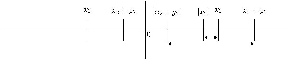
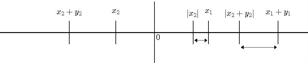
Figure 1: Case analysis in the proof of Claim 6.1

The top figure corresponds to the case where both $y_{1}$ and $y_{2}$ are non-negative, i.e. $y_{1}=y_{2}=\frac{d}{p_{Y}}\geq 0$. Notice that the distance between $\left|x_{1}+y_{1}\right|$ and $\left|x_{2}+y_{2}\right|$ is at least the distance between $\left|x_{1}\right|$ and $\left|x_{2}\right|$. This case occurs with probability $p_{Y}^{2}$.

The bottom figure corresponds to the case where $p_{Y}<\frac{1}{2}$ and $y_{1}=\frac{d}{p_{Y}}>\frac{d}{1-p_{Y}}=\left|y_{2}\right|$. Notice that in this case the distance also cannot decrease. In particular, when $p_{Y}<\frac{1}{4}$, we have $y_{1}=\frac{d}{p_{Y}}>3\frac{d}{1-p_{Y}}=3\left|y_{2}\right|$, and therefore the distance actually increases by a significant amount. This case occurs with probability $p_{Y}\left(1-p_{Y}\right)$.

1. If $p_{Y}\geq\frac{1}{2}$ then with probability at least $\frac{1}{4}$ both evaluations of $\bar{Y}$ are non-negative, in which case the distance between $\left|x_{1}\right|$ and $\left|x_{2}\right|$ can only increase:

   $${\mathrm{E}}_{y_{1},y_{2}}\left(\left|x_{1}+y_{1}\right|-\left|x_{2}+y_{2}\right|\right)^{2} \geq \Pr\left[y_{1},y_{2}\geq 0\right]\cdot\left(x_{1}+\frac{d}{p_{Y}}-\left|x_{2}+\frac{d}{p_{Y}}\right|\right)^{2}$$

   $$\geq \Pr\left[y_{1},y_{2}\geq 0\right]\cdot\left(x_{1}+\frac{d}{p_{Y}}-\left|x_{2}\right|-\frac{d}{p_{Y}}\right)^{2}$$

   $$\geq \frac{1}{4}\left(\left|x_{1}\right|-\left|x_{2}\right|\right)^{2}.$$

2. If $\frac{1}{4}\leq p_{Y}<\frac{1}{2}$ then with probability at least $\frac{1}{4}$, $y_{1}$ is non-negative; we also use $\frac{d}{p_{Y}}\geq\left|\frac{-d}{1-p_{Y}}\right|$ implies $y_{1}\geq\left|y_{2}\right|$:

   $${\mathrm{E}}_{y_{1},y_{2}}\left(\left|x_{1}+y_{1}\right|-\left|x_{2}+y_{2}\right|\right)^{2} \geq \Pr\left[y_{1}\geq 0\right]\cdot\left(\left|x_{1}\right|-\left|x_{2}\right|+y_{1}-\left|y_{2}\right|\right)^{2}$$

   $$\geq \Pr\left[y_{1}\geq 0\right]\cdot\left(\left|x_{1}\right|-\left|x_{2}\right|\right)^{2}$$

   $$\geq \frac{1}{4}\left(\left|x_{1}\right|-\left|x_{2}\right|\right)^{2}.$$

3. If $p_{Y}<\frac{1}{4}$ and $x_{1}\leq\frac{2d}{1-p_{Y}}$, we can prove the claim by focusing on the case $y_{1}\geq 0,y_{2}<0$:

   $${\mathrm{E}}_{y_{1},y_{2}}\left(\left|x_{1}+y_{1}\right|-\left|x_{2}+y_{2}\right|\right)^{2} \geq \Pr\left[y_{1}\geq 0,y_{2}<0\right]\cdot\left(x_{1}-x_{2}+\frac{d}{p_{Y}}-\frac{d}{1-p_{Y}}\right)^{2}$$ (12)

   Notice that $p_{Y}\leq\frac{1}{3}\left(1-p_{Y}\right)$ implies that

   $$\frac{d}{p_{Y}}-\frac{d}{1-p_{Y}}\geq\frac{2}{3}\cdot\frac{d}{p_{Y}}.$$

   Furthermore, since $p_{Y}\leq\frac{1}{4}$ and $1-p_{Y}\geq\frac{3}{4}$, we have that

   $$\frac{d}{p_{Y}}-\frac{d}{1-p_{Y}}\geq\frac{2}{3}\cdot\frac{\sqrt{p_{Y}}}{\frac{1}{2}}\cdot\frac{\left(\frac{3}{4}\right)^{3/2}}{\left(1-p_{Y}\right)^{3/2}}\cdot\frac{d}{p_{Y}}=\frac{\sqrt{\frac{3}{2}}}{\sqrt{p_{Y}\left(1-p_{Y}\right)}}\frac{d}{1-p_{Y}}\geq\frac{\sqrt{\frac{3}{8}}}{\sqrt{p_{Y}\left(1-p_{Y}\right)}}\left|x_{1}\right|.$$

   Plugging back into (12) we have

   $${\mathrm{E}}_{y_{1},y_{2}}\left(\left|x_{1}+y_{1}\right|-\left|x_{2}+y_{2}\right|\right)^{2} \geq \Pr\left[y_{1}\geq 0,y_{2}<0\right]\left(\frac{\sqrt{\frac{3}{8}}}{\sqrt{p_{Y}\left(1-p_{Y}\right)}}\left|x_{1}\right|\right)^{2}=\frac{3}{8}\left|x_{1}\right|^{2}.$$

4. Else, if $p_{Y}<\frac{1}{4}$ and $x_{1}>\frac{2d}{1-p_{Y}}$, we need to sum over the possible signs of $y_{1},y_{2}$, and use the fact that $\frac{d}{p_{Y}}$ is much larger than $\left|\frac{-d}{1-p_{Y}}\right|$:

   $${\mathrm{E}}_{y_{1},y_{2}}\left(\left|x_{1}+y_{1}\right|-\left|x_{2}+y_{2}\right|\right)^{2} \geq \Pr\left[y_{1}\geq 0,y_{2}\geq 0\right]\cdot\left(\left|x_{1}\right|-\left|x_{2}\right|\right)^{2}+$$

   $$\Pr\left[y_{1}\geq 0,y_{2}<0\right]\cdot\underbrace{\left(\left|x_{1}\right|-\left|x_{2}\right|+\left(\frac{d}{p_{Y}}-\frac{d}{1-p_{Y}}\right)\right)^{2}}_{\left(a\right)}+$$

   $$\Pr\left[y_{1}<0,y_{2}<0\right]\cdot\underbrace{\left(\left|x_{1}\right|-\left|x_{2}\right|-\frac{2d}{1-p_{Y}}\right)^{2}}_{\left(b\right)},$$

   where we used the condition $x_{1}>\frac{2d}{1-p_{Y}}$ in the third line.

   We have

   $$\left(a\right)\geq\left(\left|x_{1}\right|-\left|x_{2}\right|\right)^{2}+2\left(\frac{d}{p_{Y}}-\frac{d}{1-p_{Y}}\right)\left(\left|x_{1}\right|-\left|x_{2}\right|\right)$$

   and

   $$\left(b\right)\geq\frac{1}{4}\left(b\right)\geq\frac{1}{4}\left(\left(\left|x_{1}\right|-\left|x_{2}\right|\right)^{2}-2\frac{2d}{1-p_{Y}}\left(\left|x_{1}\right|-\left|x_{2}\right|\right)\right).$$

   Therefore,

   $${\mathrm{E}}_{y_{1},y_{2}}\left(\left|x_{1}+y_{1}\right|-\left|x_{2}+y_{2}\right|\right)^{2} \geq p_{Y}^{2}\left(\left|x_{1}\right|-\left|x_{2}\right|\right)^{2}+$$

   $$p_{Y}\left(1-p_{Y}\right)\left(\left(\left|x_{1}\right|-\left|x_{2}\right|\right)^{2}+2\left(\frac{d}{p_{Y}}-\frac{d}{1-p_{Y}}\right)\left(\left|x_{1}\right|-\left|x_{2}\right|\right)\right)+$$

   $$\frac{1}{4}\left(1-p_{Y}\right)^{2}\left(\left(\left|x_{1}\right|-\left|x_{2}\right|\right)^{2}-2\frac{2d}{1-p_{Y}}\left(\left|x_{1}\right|-\left|x_{2}\right|\right)\right)$$

   $$\geq\frac{1}{4}\left(\left|x_{1}\right|-\left|x_{2}\right|\right)^{2}+2d\left(\left(1-2\cdot\frac{1}{4}\right)\left(1-p_{Y}\right)-p_{Y}\right)\left(\left|x_{1}\right|-\left|x_{2}\right|\right)$$

   $$\geq\frac{1}{4}\left(\left|x_{1}\right|-\left|x_{2}\right|\right)^{2}.$$

∎

7.2 Constant absolute value: proof of Claim 6.2

We use a brute-force case analysis to prove a relative lower bound on the variance in absolute value of a sum of two variables with constant absolute values:

Claim 7.2.

(Claim 6.2) Let $\bar{X},\bar{Y}$ be balanced random variables and let $X^{\prime},Y^{\prime}$ be the constant-absolute-value approximations of $\bar{X},\bar{Y}$, respectively:

$$X^{\prime} = \mbox{sign}\left(\bar{X}+E\right)\cdot{\mathrm{E}}\left|\bar{X}+E\right|$$

$$Y^{\prime} = \mbox{sign}\left(\bar{Y}+E\right)\cdot{\mathrm{E}}\left|\bar{Y}+E\right|.$$

Then the variance of the absolute value of $X^{\prime}+Y^{\prime}-E$ is bounded by:

$${\mathrm{Var}}\left|X^{\prime}+Y^{\prime}-E\right|\geq\frac{{\mathrm{Var}}\left(X^{\prime}-E\right){\mathrm{Var}}\left(Y^{\prime}-E\right)}{16\left({\mathrm{Var}}\bar{X}+E^{2}\right)}.$$

Proof.

Denote $p_{X}=\Pr\left[\bar{X}+E\geq 0\right]$ and $d_{X}={\mathrm{E}}\left|\bar{X}+E\right|$ (and analogously for $p_{Y},d_{Y}$).

Observe that

$$d_{X}\leq\sqrt{{\mathrm{E}}\left[\left(\bar{X}+E\right)^{2}\right]}=\sqrt{{\mathrm{Var}}\left(\bar{X}+E\right)+\left({\mathrm{E}}\left[\bar{X}+E\right]\right)^{2}}=\sqrt{{\mathrm{Var}}\bar{X}+E^{2}}.$$

Thus we can bound $\left(1-p_{X}\right)p_{X}$ from below by:

$${\mathrm{Var}}X^{\prime}=\left(2d_{X}\right)^{2}\Pr\left[X^{\prime}\leq 0\right]\Pr\left[X^{\prime}>0\right]\leq 4\left({\mathrm{Var}}\bar{X}+E^{2}\right)\left(1-p_{X}\right)p_{X}$$

$$\left(1-p_{X}\right)p_{X}\geq\frac{{\mathrm{Var}}X^{\prime}}{4\left({\mathrm{Var}}\bar{X}+E^{2}\right)}.$$ (13)

Also, for $Y^{\prime}$ we have

$${\mathrm{Var}}Y^{\prime}=p_{Y}\cdot\left(1-p_{Y}\right)\left(2d_{Y}\right)^{2}.$$

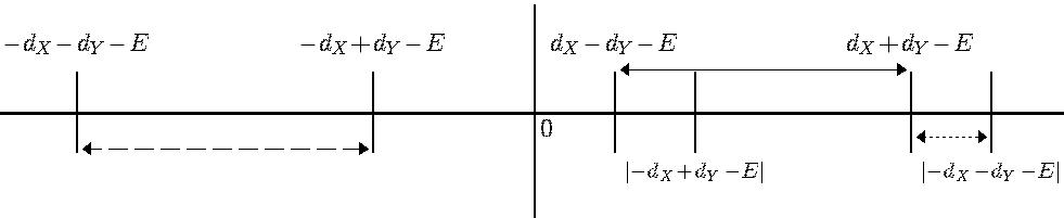
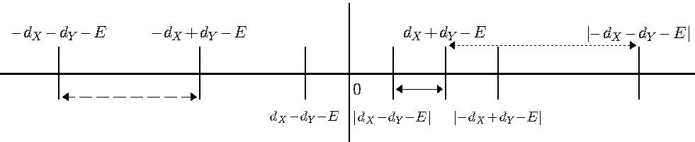
Figure 2: Case analysis in the proof of Claim 6.2

• With probability $2\left(1-p_{X}\right)^{2}\cdot\left(1-p_{Y}\right)p_{Y}$ both $x$’s are negative, and $y$’s are of opposite signs. Notice that since we assume $E\geq 0$ and $d_{X}\geq d_{Y}$, the distance between $\left|-d_{X}-d_{Y}-E\right|$ and $\left|-d_{X}+d_{Y}-E\right|$ is the same as the distance between $-d_{X}-d_{Y}-E$ and $-d_{X}+d_{Y}-E$ (marked by dashed line on both figures); it is therefore always $2d_{Y}$ .

• With probability $2p_{X}^{2}\cdot\left(1-p_{Y}\right)p_{Y}$ both $x$’s are positive, and $y$’s are of opposite signs. Notice that the distance between $\left|d_{X}+d_{Y}-E\right|$ and $\left|d_{X}-d_{Y}-E\right|$ (marked by the solid lines) is either $2d_{Y}$ (as in the top figure) or $\left|2d_{X}-2E\right|$ when $d_{X}-d_{Y}-E\leq 0$ (as in the bottom figure).

• With probability $2\left(1-p_{X}\right)p_{X}\cdot\left(1-p_{Y}\right)p_{Y}$ the $x$’s and $y$’s are of correlated signs. Notice that the distance between $\left|d_{X}+d_{Y}-E\right|$ and $\left|-d_{X}-d_{Y}-E\right|$ (marked by the dotted lines) is either $2E$ (as in both figures) or $2d_{X}+2d_{Y}$ when $d_{X}+d_{Y}-E\leq 0$ (not shown).

Assume without loss of generality that $d_{Y}<d_{X}$ and $E>0$. Recall (Fact 2.4) that we can write the variance in terms of the expected squared distance between evaluations. Then, summing over the different possible signs of $X^{\prime}$ and $Y^{\prime}$ we have

$${\mathrm{Var}}\left|X^{\prime}+Y^{\prime}-E\right| = \frac{1}{2}{\mathrm{E}}_{x_{1},x_{2},y_{1},y_{2}\sim X^{\prime}\times X^{\prime}\times Y^{\prime}\times Y^{\prime}}\left(\left|x_{1}+y_{1}-E\right|-\left|x_{2}+y_{2}-E\right|\right)^{2}$$

$$\geq \left(1-p_{X}\right)^{2}\cdot\left(1-p_{Y}\right)p_{Y}\cdot\left(\left|-d_{X}-d_{Y}-E\right|-\left|-d_{X}+d_{Y}-E\right|\right)^{2}+$$

$$p_{X}^{2}\cdot\left(1-p_{Y}\right)p_{Y}\cdot\left(\left|d_{X}-d_{Y}-E\right|-\left|d_{X}+d_{Y}-E\right|\right)^{2}+$$

$$\left(1-p_{X}\right)p_{X}\cdot\left(1-p_{Y}\right)p_{Y}\cdot\left(\left|-d_{X}-d_{Y}-E\right|-\left|d_{X}+d_{Y}-E\right|\right)^{2}$$

$$\geq \left(\left(1-p_{X}\right)^{2}+p_{X}^{2}\right)\cdot\left(1-p_{Y}\right)p_{Y}\cdot\underbrace{\min\left\{\left|2d_{X}-2E\right|,2d_{Y}\right\}^{2}}_{\left(a\right)}+$$

$$\left(1-p_{X}\right)p_{X}\cdot p_{Y}\left(1-p_{Y}\right)\cdot\underbrace{\min\left\{2E,2d_{X}+2d_{Y}\right\}^{2}}_{\left(b\right)}$$

(Where the first inequality follows by taking the expectation over the different possible signs of $X^{\prime}$, $Y^{\prime}$ (see also Figure 2); the second follows by taking the minimum over the possible signs of the quantities in absolute values;)

We next claim that

$$\left(a\right)+\left(b\right)\geq d_{Y}^{2}$$ (14)

If $2E\geq d_{Y}$, (14) is immediate. If $2E<d_{Y}$, then (14) follows because $2d_{X}-2E\geq d_{x}\geq d_{Y}$.

Therefore,

$${\mathrm{Var}}\left|X^{\prime}+Y^{\prime}-E\right| \geq \left(1-p_{X}\right)p_{X}\cdot p_{Y}\left(1-p_{Y}\right)\cdot d_{Y}^{2}$$

$$\geq \frac{{\mathrm{Var}}X^{\prime}}{4\left({\mathrm{Var}}\bar{X}+E^{2}\right)}\cdot p_{Y}\left(1-p_{Y}\right)\cdot\frac{\left(2d_{Y}\right)^{2}}{4}$$

$$= \frac{{\mathrm{Var}}X^{\prime}}{16\left({\mathrm{Var}}\bar{X}+E^{2}\right)}\cdot{\mathrm{Var}}Y^{\prime}$$

$$= \frac{{\mathrm{Var}}\left(X^{\prime}-E\right){\mathrm{Var}}\left(Y^{\prime}-E\right)}{16\left({\mathrm{Var}}\bar{X}+E^{2}\right)}.$$

(Where the first inequality follows from (14) and $\left(1-p_{X}\right)^{2}+p_{X}^{2}>\left(1-p_{X}\right)p_{X}$; and the second inequality follows by (13).) ∎

8 Tightness of results

8.1 Tightness of the main result

The premise of main result, corollary 4.1, requires $f$ to be $\left(\epsilon\cdot{\mathrm{Var}}f\right)$-close to a sum of independent functions. One may hope to avoid this factor of ${\mathrm{Var}}f$ and achieve a constant ratio between $\epsilon$ in the premise and $\left(K\cdot\epsilon\right)$ in the conclusion, as in the FKN Theorem. However, we show that the dependence on ${\mathrm{Var}}f$ is necessary.

lemmama.

(Lemma 4.1) Corollary 4.1 is tight up to a constant factor. In particular, the factor ${\mathrm{Var}}f$ is necessary.

More precisely, there exists a sequence of functions $f^{\left(m\right)}\colon\left\{\pm 1\right\}^{2m}\rightarrow\left\{\pm 1\right\}$ and partitions $\left(I_{1}^{\left(m\right)},I_{2}^{\left(m\right)}\right)$ such that the restrictions $\left(f_{1}^{\left(m\right)},f_{2}^{\left(m\right)}\right)$ of $f^{\left(m\right)}$ to variables in $I_{j}^{\left(m\right)}$ satisfy

$$\sum_{S\colon\exists j,\,S\subseteq I_{j}^{\left(m\right)}}\hat{f}{}^{2}\left(S\right)=1-O\left(2^{-m}\cdot{\mathrm{Var}}f\right).$$

but for every $j\in\left\{1,2\right\}$

$$\left\|f^{\left(m\right)}-f_{j}^{\left(m\right)}-\widehat{f^{\left(m\right)}}\left(\emptyset\right)\right\|_{2}^{2}=\Theta\left(2^{-m}\right)=\omega\left(2^{-m}\cdot{\mathrm{Var}}f\right).$$

Proof.

By example. Let

$$X = \bigwedge_{i=1}^{m}x_{i}$$

$$Y = \bigwedge_{i=1}^{m}y_{i}$$

$$f = X\vee Y,$$

where we think of $-1$ as “true” and $1$ as “false”.

The variance of $f$ is $\Theta\left(2^{-m}\right)$:

$${\mathrm{Var}}f=4\Pr\left[f=1\right]\Pr\left[f=-1\right]=4\left(1-\Theta\left(2^{-m}\right)\right)\Theta\left(2^{-m}\right)=\Theta\left(2^{-m}\right).$$

Also, $f$ is $O\left(2^{-2m}\right)$-close to a sum of independent functions:

$$f = \frac{X+Y+X\cdot Y-1}{2}$$

$$\left\|f-\left(X+Y-1\right)\right\|_{2}^{2} = \left\|\frac{\left(X-1\right)\left(Y-1\right)}{2}\right\|_{2}^{2}=4\cdot 2^{-2m}.$$

Yet, $f$ is $\Omega\left(2^{-m}\right)$-far from any function that depends on either only the $x_{i}$’s or only the $y_{i}$’s. ∎

8.2 Tightness of Lemma 5.2

Lemma 5.2 compares the variance of the absolute value of a sum of independent variables, to the variance of the absolute value of each variable. Since both sides of the inequality consider absolute values, it may seem as if we should only be increasing the variation on the left side by summing independent variables. In particular, one may hope that the inequality should hold trivially, with $K_{0}=1$. We show that this is not the case.

Claim 8.1.

(Claim 5.1) A non-trivial constant is necessary for Lemma 5.2. More precisely, there exist two independent balanced random variables $\bar{X},\bar{Y}$, such that the following inequality does not hold for any value $K_{0}<4/3$:

$${\mathrm{Var}}\left|\bar{X}+\bar{Y}\right|\geq\frac{\max\left\{{\mathrm{Var}}\left|\bar{X}\right|,{\mathrm{Var}}\left|\bar{Y}\right|\right\}}{K_{0}}$$

(In particular, it is interesting to note that $K_{0}>1$.)

Proof.

By example. Let

$$\Pr\left[X=0\right] = \frac{1}{2}$$

$$\Pr\left[X=\pm 2\right] = \frac{1}{4}$$

$$\Pr\left[Y=\pm 1\right] = \frac{1}{2}.$$

Then we have that

$${\mathrm{E}}X={\mathrm{E}}Y=0$$

$$\Pr\left[\left|X+Y\right|=1\right] = \frac{3}{4}$$

$$\Pr\left[\left|X+Y\right|=3\right] = \frac{1}{4},$$

and therefore

$${\mathrm{Var}}\left|X+Y\right|=\frac{3}{4}=\frac{3}{4}{\mathrm{Var}}\left|X\right|.$$

∎

9 Conjectures and extensions

While the dependence on the variance in Corollary 4.1 is tight, it seems counter-intuitive. We believe that it is possible to come up with a structural characterization instead.

Observe that the function used for the counter example in Lemma 4.1 is essentially the (non-balanced) tribes function, i.e. $OR$ of two $AND$’s. All the extreme examples we have discovered so far have a similar structure of an independent Boolean function on each subset of the variables (e.g. $AND$ on a subset of the variables), and then a “central” Boolean function that takes as inputs the outputs of the independent functions (e.g. $OR$ of all the $AND$’s).

We conjecture that such a composition of Boolean functions is essentially the only way to construct counterexamples to the “naive extension” of the FKN Theorem. In other words, if a Boolean function is close to linear with respect to a partition of the variables, then it is close to the application of a central Boolean function $g$ on the outputs of independent Boolean functions $g_{j}$’s, one over each subset $I_{j}$. Formally,

Conjecture 9.1.

Let $f\colon\left\{\pm 1\right\}^{m}\rightarrow\left\{\pm 1\right\}$ be a Boolean function, $\left(I_{j}\right)_{j=1}^{n}$ a partition of $\left[m\right]$. Suppose that $f$ is concentrated on coefficients that do not cross the partition, i.e.:

$$\sum_{S\colon\exists j,\,S\subseteq I_{j}}\hat{f}{}^{2}\left(S\right)\geq 1-\epsilon.$$

Then there exist a “central” Boolean function $g\colon\left\{\pm 1\right\}^{n}\rightarrow\left\{\pm 1\right\}$ and a Boolean function on each subset $h_{j}\colon\left\{\pm 1\right\}^{\left|I_{j}\right|}\rightarrow\left\{\pm 1\right\}$ such that the composition of $g$ with the $h_{j}$’s is a good approximation of $f$. I.e. for some universal constant $K$,

$$\left\|f\left(X\right)-g\left(h_{1}\left(\left(x_{i}\right)_{i\in I_{1}}\right),h_{2}\left(\left(x_{i}\right)_{i\in I_{2}}\right),\dots,h_{n}\left(\left(x_{i}\right)_{i\in I_{n}}\right)\right)\right\|_{2}^{2}\leq K\cdot\epsilon.$$

Intuitively, this conjecture claims that the central function only needs to know one bit of information on each subset in order to approximate $f$.

We believe that such a conjecture could have useful applications because one can often deduce properties of the composition of independent functions $f=g\left(h\left(x_{I_{1}}\right),h\left(x_{I_{2}}\right),\dots,h\left(x_{I_{n}}\right)\right)$ from the properties of the composed functions $g$ and $h$. For example if $f$, $g$, and $h$ are as above, then the total influence of $f$ is the product of the total influences of $g$ and $h$.

In fact, we believe that an even stronger claim holds. It seems that for all the Boolean functions that are almost linear with respect to a partition of the variables, the “central” function $g$ is either an $OR$ or an $AND$ of some of the functions on the subsets $h_{j}$. Formally,

Conjecture 9.2.

(Stronger variant) Let $f\colon\left\{\pm 1\right\}^{m}\rightarrow\left\{\pm 1\right\}$ be a Boolean function, $\left(I_{j}\right)_{j=1}^{n}$ a partition of $\left[m\right]$. Suppose that $f$ is concentrated on coefficients that do not cross the partition, i.e.:

$$\sum_{S\colon\exists j,\,S\subseteq I_{j}}\hat{f}{}^{2}\left(S\right)\geq 1-\epsilon.$$

Then there exist Boolean functions $h_{j}\colon\left\{\pm 1\right\}^{\left|I_{j}\right|}\rightarrow\left\{\pm 1\right\}$ for each $j\in\left[n\right]$ such that either the $OR$ or the $AND$ of those $h_{j}$’s is a good approximation of $f$. I.e. for some universal constant $K$,

$$\left\|f\left(X\right)-OR_{j\in\left[n\right]}\left(h_{j}\left(\left(x_{i}\right)_{i\in I_{j}}\right)\right)\right\|_{2}^{2}\leq K\cdot\epsilon$$

-or-

$$\left\|f\left(X\right)-AND_{j\in\left[n\right]}\left(h_{j}\left(\left(x_{i}\right)_{i\in I_{j}}\right)\right)\right\|_{2}^{2}\leq K\cdot\epsilon.$$

Acknowledgement.

An earlier version of this paper appeared before as the Masters thesis of the first author.

We are grateful to anonymous referees for pointing out errors in a previous draft, as well as many helpful comments and suggestions.

Appendix A Proofs of preliminary facts

Below, we bring missing proofs of facts from Section 2. All these proofs can be found elsewhere (e.g. [28]), and are brought here only for completeness.

Fact A.1.

(Fact 2.2)

$$\left\|f-g\right\|_{2}^{2}=\sum\left(\widehat{f}\left(S\right)-\widehat{g}\left(S\right)\right)^{2}.$$

Proof.

$$\left\|f-g\right\|_{2}^{2}=\sum\left(\widehat{f-g}\left(S\right)\right)^{2}=\sum\left(\widehat{f}\left(S\right)-\widehat{g}\left(S\right)\right)^{2}.$$

∎

Fact A.2.

(Fact 2.3)

$${\mathrm{Var}}f=\sum_{S\neq\emptyset}\widehat{f}\left(S\right)^{2}.$$

Proof.

$${\mathrm{Var}}f = {\mathrm{E}}\left[f^{2}\right]-\left({\mathrm{E}}f\right)^{2}$$

$$= {\mathrm{E}}\left[\left(\sum_{S}\widehat{f}\left(S\right)\chi_{S}\right)^{2}\right]-\left({\mathrm{E}}\sum_{S}\widehat{f}\left(S\right)\chi_{S}\right)^{2}$$

$$= \left(\sum_{S,T}\widehat{f}\left(S\right)\widehat{f}\left(T\right){\mathrm{E}}\chi_{S}\chi_{T}\right)-\left(\sum_{S}\widehat{f}\left(S\right){\mathrm{E}}\chi_{S}\right)^{2}$$

$$= \left(\sum_{S}\widehat{f}\left(S\right)^{2}\right)-\left(\widehat{f}\left(\emptyset\right)\right)^{2}.$$

∎

Fact A.3.

(Fact 2.4) For any random variable X,

$${\mathrm{Var}}X=\frac{1}{2}\cdot{\mathrm{E}}_{x_{1},x_{2}\sim X\times X}\left(x_{1}-x_{2}\right)^{2}.$$

Proof.

$${\mathrm{E}}_{x_{1},x_{2}\sim X\times X}\left(x_{1}-x_{2}\right)^{2}={\mathrm{E}}x_{1}^{2}+{\mathrm{E}}x_{2}^{2}-2{\mathrm{E}}x_{1}x_{2}=2\left({\mathrm{E}}X^{2}-\left({\mathrm{E}}X\right)^{2}\right)=2{\mathrm{Var}}X.$$

∎

Fact A.4.

(Fact 2.5)

$${\mathrm{Var}}X=\left\|X-{\mathrm{E}}X\right\|_{2}^{2}.$$

Proof.

$${\mathrm{E}}\left[X^{2}\right]-\left({\mathrm{E}}X\right)^{2}={\mathrm{E}}\left[X^{2}\right]-2{\mathrm{E}}\left[X{\mathrm{E}}X\right]+{\mathrm{E}}\left[\left({\mathrm{E}}X\right)^{2}\right]={\mathrm{E}}\left[\left(X-{\mathrm{E}}X\right)^{2}\right].$$

∎

Fact A.5.

(Fact 2.6)

$${\mathrm{Var}}X=\min_{E\in\mathbb{R}}\left\|X-E\right\|_{2}^{2}.$$

Proof.

Differentiate twice with respect to $E$:

$$\frac{d}{dE}\left\|X-E\right\|_{2}^{2} = 2\left({\mathrm{E}}X-E\right)$$

$$\frac{d^{2}}{dE^{2}}\left\|X-E\right\|_{2}^{2} = -2.$$

∎

References

- [1] Noga Alon, Irit Dinur, Ehud Friedgut, and Benny Sudakov. Graph products, Fourier analysis and spectral techniques. GAFA, 14:913–940, 2004.
- [2] Nikhil Bansal and Subhash Khot. Optimal long code test with one free bit. In FOCS, pages 453–462, 2009.
- [3] William Beckner. Inequalities in Fourier analysis. Annals of Mathematics, 102:159–182, 1975.
- [4] Mihir Bellare, Oded Goldreich, and Madhu Sudan. Free Bits, PCPs, and Nonapproximability-Towards Tight Results. SIAM J. Comput., 27(3):804–915, 1998.
- [5] Aline Bonami. ï¿œtude des coefficients de Fourier des fonctions de . Annales de l’institut Fourier, 20:335–402, 1970.
- [6] J. Bourgain. On the distribution of the Fourier spectrum of Boolean functions. Israel Journal of Mathematics, 131:269–276, 2002.
- [7] Shuchi Chawla, Robert Krauthgamer, Ravi Kumar, Yuval Rabani, and D. Sivakumar. On the hardness of approximating multicut and sparsest-cut. Computational Complexity, 15(2):94–114, 2006.
- [8] Irit Dinur. The PCP theorem by gap amplification. J. ACM, 54(3):12, 2007.
- [9] Irit Dinur and Shmuel Safra. On the hardness of approximating minimum vertex-cover. Annals of Mathematics, 162(1)(5):439–485, 2005.
- [10] David Ellis, Yuval Filmus, and Ehud Friedgut. A quasi-stability result for dictatorships in . Cobminatorica. To appear.
- [11] David Ellis, Yuval Filmus, and Ehud Friedgut. A stability result for balanced dictatorships in s. Random Struct. Algorithms, 46(3):494–530, 2015.
- [12] Dvir Falik and Ehud Friedgut. Between Arrow and Gibbard-Satterthwaite; A representation theoretic approach. Israel Journal of Mathematics, 201(1):247–297, 2014.
- [13] Ehud Friedgut. Boolean functions with low average sensitivity depend on few coordinates. Combinatorica, 18(1):27–35, 1998.
- [14] Ehud Friedgut. On the measure of intersecting families, uniqueness and stability. Combinatorica, 28(5):503–528, 2008.
- [15] Ehud Friedgut, Gil Kalai, and Assaf Naor. Boolean functions whose Fourier transform is concentrated on the first two levels. Advances in Applied Mathematics, 29(3):427 – 437, 2002. Note: we rely on a simplification by Guy Kindler which can be found in the online version of this article at http://www.ma.huji.ac.il/~kalai/fkn.pdf.
- [16] Mahya Ghandehari and Hamed Hatami. Fourier analysis and large independent sets in powers of complete graphs. J. Comb. Theory, Ser. B, 98(1):164–172, 2008.
- [17] Johan Håstad. Clique is hard to approximate within . In Proceedings of the 37th Annual Symposium on Foundations of Computer Science, FOCS ’96, pages 627–, Washington, DC, USA, 1996. IEEE Computer Society.
- [18] Johan Håstad. Some optimal inapproximability results. J. ACM, 48(4):798–859, July 2001.
- [19] Jacek Jendrej, Krzysztof Oleszkiewicz, and Jakub O. Wojtaszczyk. On some extensions to the FKN theorem. In Phenomena in high dimensions in geometric analysis, random matrices, and computational geometry, 2012.
- [20] Jacek Jendrej, Krzysztof Oleszkiewicz, and Jakub O. Wojtaszczyk. On some extensions of the FKN theorem. Theory of Computing, To appear.
- [21] Gil Kalai. A Fourier-theoretic perspective on the Condorcet paradox and Arrow’s theorem. Technical Report 3, 2002.
- [22] Subhash Khot and Oded Regev. Vertex cover might be hard to approximate to within 2-. J. Comput. Syst. Sci., 74(3):335–349, 2008.
- [23] Subhash Khot and Nisheeth K. Vishnoi. The unique games conjecture, integrality gap for cut problems and embeddability of negative type metrics into . In FOCS, pages 53–62, 2005.
- [24] Guy Kindler. Property Testing, PCP, and Juntas. PhD thesis, Tel-Aviv University, 2002.
- [25] Guy Kindler and Ryan O’Donnell. Gaussian noise sensitivity and Fourier tails. In IEEE Conference on Computational Complexity, pages 137–147, 2012.
- [26] Ashley Montanaro and Tobias Osborne. Quantum boolean functions. Chicago J. Theor. Comput. Sci., 2010, 2010.
- [27] Piotr Nayar. FKN theorem on the biased cube. CoRR, arXiv:1311.3179, 11 2013.
- [28] Ryan O’Donnell. Analysis of Boolean Functions. Cambridge University Press, 2014.
- [29] Jakub Onufry Wojtaszczyk. Sums of independent variables approximating a boolean function. Submitted, 2010.