Differentially Private Average Consensus: Obstructions, Trade-Offs, and Optimal Algorithm Design

Abstract

This paper studies the multi-agent average consensus problem under the requirement of differential privacy of the agents’ initial states against an adversary that has access to all the messages. We first establish that a differentially private consensus algorithm cannot guarantee convergence of the agents’ states to the exact average in distribution, which in turn implies the same impossibility for other stronger notions of convergence. This result motivates our design of a novel differentially private Laplacian consensus algorithm in which agents linearly perturb their state-transition and message-generating functions with exponentially decaying Laplace noise. We prove that our algorithm converges almost surely to an unbiased estimate of the average of agents’ initial states, compute the exponential mean-square rate of convergence, and formally characterize its differential privacy properties. We show that the optimal choice of our design parameters (with respect to the variance of the convergence point around the exact average) corresponds to a one-shot perturbation of initial states and compare our design with various counterparts from the literature. Simulations illustrate our results.

1 Introduction

The social adoption of new technologies in networked cyberphysical systems relies heavily on the privacy preservation of individual information. Social networking, the power grid, and smart transportation are only but a few examples of domains in need of privacy-aware design of control and coordination strategies. In these scenarios, the ability of a networked system to fuse information, compute common estimates of unknown quantities, and agree on a common view of the world is critical. Motivated by these observations, this paper studies the multi-agent average consensus problem, where a group of agents seek to agree on the average of their individual values by only interchanging information with their neighbors. This problem has numerous applications in synchronization, network management, and distributed control/computation/optimization. In the context of privacy preservation, the notion of differential privacy has gained significant popularity due to its rigorous formulation and proven security properties, including resilience to post-processing and side information, and independence from the model of the adversary. Roughly speaking, a strategy is differentially private if the information of an agent has no significant effect on the aggregate output of the algorithm, and hence its data cannot be inferred by an adversary from its execution. This paper is a contribution to the emerging body of research that studies privacy preservation in cooperative network systems, specifically focused on gaining insight into the achievable trade-offs between privacy and performance in multi-agent average consensus.

Literature Review: The problem of multi-agent average consensus has been a subject of extensive research in networked systems and it is impossible to survey here the vast amount of results in the literature. We provide (Bullo et al., 2009; Ren and Beard, 2008; Mesbahi and Egerstedt, 2010; Olfati-Saber et al., 2007) and the references therein as a starting point for the interested reader. In cyberphysical systems, privacy at the physical layer provides protection beyond the use of higher-level encryption-based techniques. Information-theoretic approaches to privacy at the physical layer have been actively pursued (Gündüz et al., 2010; Mukherjee et al., 2014). Recently, these ideas have also been utilized in the context of control (Tanaka and Sandberg, 2015). The paper (Mukherjee et al., 2014) also surveys the more recent game-theoretic approach to the topic. In computer science, the notion of differential privacy, first introduced in (Dwork et al., 2006; Dwork, 2006), and the design of differentially private mechanisms have been widely studied in the context of privacy preservation of databases. The work (Dwork and Roth, 2014) provides a recent comprehensive treatment. A well-known advantage of differential privacy over other notions of privacy is its immunity to post-processing and side information, which makes it particularly well-suited for multi-agent scenarios where agents do not fully trust each other and/or the communication channels are not fully secure. While secure multi-party computation also deals with scenarios where no trust exists among agents, the maximum number of agents that can collude (without the privacy of others being breached) is bounded, whereas using differential privacy provides immunity against arbitrary collusions (Kairouz et al., 2015; Pettai and Laud, 2015). As a result, differential privacy has been adopted by recent works in a number of areas pertaining to networked systems, such as control (Huang et al., 2012, 2014; Wang et al., 2014), estimation (Ny and Pappas, 2014), and optimization (Han et al., 2014; Huang et al., 2015; Nozari et al., 2017). Of relevance to our present work, the paper (Huang et al., 2012) studies the average consensus problem with differentially privacy guarantees and proposes an adjacency-based distributed algorithm with decaying Laplace noise and mean-square convergence. The algorithm preserves the differential privacy of the agents’ initial states but the expected value of its convergence point depends on the network topology and may not be the exact average, even in expectation. By contrast, the algorithm proposed in this work enjoys almost sure convergence, asymptotic unbiasedness, and an explicit characterization of its convergence rate. Our results also allow individual agents to independently choose their level of privacy. The problem of privacy-preserving average consensus has also been studied using other notions of privacy. The work (Manitara and Hadjicostis, 2013) builds on (Kefayati et al., 2007) to let agents have the option to add to their first set of transmitted messages a zero-sum noise sequence with finite random length, which in turn allows the coordination algorithm to converge to the exact average of their initial states. As long as an adversary cannot listen to the transmitted messages of an agent as well as all its neighbors, the privacy of that agent is preserved, in the sense that different initial conditions may produce the same transmitted messages. This idea is further developed in (Mo and Murray, 2014, 2015), where agents add an infinitely-long exponentially-decaying zero-sum sequence of Gaussian noise to their transmitted messages. The algorithm has guaranteed mean-square convergence to the average of the agents’ initial states and preserves the privacy of the nodes whose messages and those of their neighbors are not listened to by the malicious nodes, in the sense that the maximum-likelihood estimate of their initial states has nonzero variance. Finally, (Duan et al., 2015) considers the problem of privacy preserving maximum consensus.

Statement of Contributions: We study the average consensus problem where a group of agents seek to compute and agree on the average of their local variables while seeking to keep them differentially private against an adversary with potential access to all group communications. This privacy requirement also applies to the case where each agent wants to keep its initial state private against the rest of the group (e.g., due to the possibility of communication leakages). The main contributions of this work are the characterization and optimization of the fundamental trade-offs between differential privacy and average consensus. Our first contribution is the formulation and formal proof of a general impossibility result. We show that as long as a coordination algorithm is differentially private, it is impossible to guarantee the convergence of agents’ states to the average of their initial values, even in distribution. This result automatically implies the same impossibility result for stronger notions of convergence. Motivated by it, our second contribution is the design of a linear Laplacian-based consensus algorithm that achieves average consensus in expectation —the most that one can expect. We prove the almost sure convergence and differential privacy of our algorithm and characterize its accuracy and convergence rate. Our final contribution is the computation of the optimal values of the design parameters to achieve the most accurate consensus possible. Letting the agents fix a (local) desired value of the privacy requirement, we minimize the variance of the algorithm convergence point as a function of the noise-to-state gain and the amplitude and decay rate of the noise. We show that the minimum variance is achieved by the one-shot perturbation of the initial states by Laplace noise. This result reveals the optimality of one-shot perturbation for static average consensus, previously (but implicitly) shown in the sense of information-theoretic entropy. Various simulations illustrate our results.

2 Preliminaries

This section introduces notations and basic concepts. We denote the set of reals, positive reals, non-negative reals, positive integers, and nonnegative integers by , $\mathbb{R}_{>0}$, $\mathbb{R}_{\geq 0}$, ${\mathbb{N}}$, and ${\mathbb{Z}}_{\geq 0}$, respectively. We denote by $\|\cdot\|$ the Euclidean norm. We let $({}^{n})^{\mathbb{N}}$ denote the space of vector-valued sequences in ⁿ. For $\{x(k)\}_{k=0}^{\infty}\in({}^{n})^{\mathbb{N}}$, we use the shorthand notation $\mathbf{x}=\{x(k)\}_{k=0}^{\infty}$ and $\mathbf{x}_{k}=\{x(j)\}_{j=0}^{k}$. $I_{n}\in{}^{n\times n}$ and $\mathbf{1}_{n}\in{}^{n}$ denote the identity matrix and the vector of ones, respectively. For $x\in{}^{n}$, $\operatorname{Ave}(x)=\frac{1}{n}\mathbf{1}_{n}^{T}x$ denotes the average of its components. We let $\Pi_{n}=\frac{1}{n}\mathbf{1}_{n}\mathbf{1}_{n}^{T}$. Note that $\Pi_{n}$ is diagonalizable, has one eigenvalue equal to $1$ with eigenspace

$$\real\mathbf{1}_{n}\triangleq\{a\mathbf{1}_{n}\mid a\in\real\},$$

and all other eigenvalues equal $0$. For a vector space $V\subset{}^{n}$, we let $V^{\perp}$ denote the vector space orthogonal to $V$. A matrix $A\in{}^{n\times n}$ is stable if all its eigenvalues have magnitude strictly less than 1. A function $\gamma:[0,\infty)\to[0,\infty)$ belongs to class $\mathcal{K}$ if it is continuous and strictly increasing and $\gamma(0)=0$. Similarly, a function $\beta:[0,\infty)\times[0,\infty)\to[0,\infty)$ belongs to class $\mathcal{K}\mathcal{L}$ if $\beta(\cdot,s)$ belongs to class $\mathcal{K}$ for any $s\in[0,\infty)$ and $\beta(r,\cdot)$ is decreasing and $\lim_{s\to\infty}\beta(r,s)=0$ for any $r\in[0,\infty)$. For $q\in(0,1)$, the Euler function is given by $\varphi(q)=\prod_{k=1}^{\infty}(1-q^{k})>0$. Note that

$$\lim_{k\to\infty}\prod_{j=k}^{\infty}(1-q^{j})=\lim_{k\to\infty}\frac{\varphi(q)}{\prod_{j=1}^{k-1}(1-q^{j})}=1.$$

For a function $f:X\to Y$ and sets $A\subseteq X$ and $B\subseteq Y$, we use $f(A)=\{f(x)\in Y|x\in A\}$ and $f^{-1}(B)=\{x\in X|f(x)\in B\}$. In general, $f(f^{-1}(B))\subseteq B$. Finally, for any topological space $X$, we denote by $\mathcal{B}(X)$ the set of Borel subsets of $X$.

2.1 Graph Theory

We present some useful notions on algebraic graph theory following (Bullo et al., 2009). Let $\mathcal{G}=(V,E,A)$ denote a weighted undirected graph with vertex set $V$ of cardinality $n$, edge set $E\subset V\times V$, and symmetric adjacency matrix $A\in\mathbb{R}_{\geq 0}^{n\times n}$. A path from $i$ to $j$ is a sequence of vertices starting from $i$ and ending in $j$ such that any pair of consecutive vertices is an edge. The set of neighbors $\mathcal{N}_{i}$ of $i$ is the set of nodes $j$ such that $(i,j)\in E$. A graph is connected if for each node there exists a path to any other node. The weighted degree matrix is the diagonal matrix $D\in{}^{n\times n}$ with diagonal $A\mathbf{1}_{n}$. The Laplacian is $L=D-A$ and has the following properties:

• $L$ is symmetric and positive semi-definite;

• $L\mathbf{1}_{n}=0$ and $\mathbf{1}_{n}^{T}L=0$, i.e., $0$ is an eigenvalue of $L$ corresponding to the eigenspace $\real\mathbf{1}_{n}$;

• $\mathcal{G}$ is connected if and only if $\text{rank}(L)=n-1$, so $0$ is a simple eigenvalue of $L$;

• All eigenvalues of $L$ belong to $[0,2d_{\text{max}}]$, where $d_{\text{max}}$ is the largest element of $D$.

For convenience, we define $L_{\text{cpt}}=I_{n}-\Pi_{n}$.

2.2 Probability Theory

Here we briefly review basic notions on probability following (Papoulis and Pillai, 2002; Durrett, 2010). Consider a probability space $(\Omega,\Sigma,\mathbb{P})$. If $E,F\in\Sigma$ are two events with $E\subseteq F$, then $\mathbb{P}\{E\}\leq\mathbb{P}\{F\}$. For simplicity, we may sometimes denote events of the type $E_{p}=\{\omega\in\Omega\mid p(\omega)\}$ by $\{p\}$, where $p$ is a logical statement on the elements of $\Omega$. Clearly, for two statements $p$ and $q$,

$$(p\Rightarrow q)\Rightarrow\left(\mathbb{P}\{p\}\leq\mathbb{P}\{q\}\right).$$ (1)

A random variable is a measurable function $X:\Omega\to\real$. For any $N\in\mathbb{R}_{>0}$ and any random variable $X$ with finite expected value $\mu$ and finite nonzero variance $\sigma^{2}$, Chebyshev’s inequality states that

$$\mathbb{P}\{\lvert X-\mu\rvert\geq N\sigma\}\leq\frac{1}{N^{2}}.$$ (2)

For a random variable $X$, let $\mathbb{E}[X]$ and $F_{X}$ denote its expectation and cumulative distribution function, respectively. A sequence of random variables $\{X_{k}\}_{k\in{\mathbb{Z}}_{\geq 0}}$ converges to a random variable $X$

• almost surely (a.s.) if $\mathbb{P}\{\lim_{k\to\infty}X_{k}=X\}=1$;

• in mean square if $\mathbb{E}[X_{k}^{2}],\mathbb{E}[X^{2}]<\infty$ for all $k\in{\mathbb{Z}}_{\geq 0}$ and $\lim_{k\to\infty}\mathbb{E}[(X_{k}-X)^{2}]=0$;

• in probability if $\lim_{k\to\infty}\mathbb{P}\{\lvert X_{k}-X\rvert<\upsilon\}=1$ for any $\upsilon>0$;

• in distribution or weakly if $\lim_{k\to\infty}F_{X_{k}}(x)=F_{X}(x)$ for any $x\in\real$ at which $F_{X}$ is continuous.

Almost sure convergence and convergence in mean square imply convergence in probability, which itself implies convergence in distribution. Moreover, if $\mathbb{P}\{\lvert X_{k}\rvert\leq\bar{X}\}=1$ for all $k\in{\mathbb{Z}}_{\geq 0}$ and some fixed random variable $\bar{X}$ with $\mathbb{E}[\bar{X}^{2}]<\infty$, then convergence in probability implies mean square convergence, and if $X$ is a constant, then convergence in distribution implies convergence in probability.

A zero-mean random variable $X$ has Laplace distribution with scale $b\in\mathbb{R}_{>0}$, denoted $X\sim\text{Lap}(b)$, if its pdf is given by $\mathcal{L}(x;b)\triangleq\frac{1}{2b}e^{-\frac{|x|}{b}}$ for any $x\in\real$. It is easy to see that $\lvert X\rvert$ has exponential distribution with rate $\lambda=\frac{1}{b}$.

2.3 Input-to-State Stability of Discrete-Time Systems

This section briefly describes notions of robustness for discrete-time systems following (Jiang and Wang, 2001). Consider a discrete-time system of the form

$$x(k+1)=f(x(k),u(k)),$$ (3)

where $u:{\mathbb{Z}}_{\geq 0}\to{}^{m}$ is a disturbance input, $x:{\mathbb{Z}}_{\geq 0}\to{}^{n}$ is the state, and $f:{}^{n}\times{}^{m}\to{}^{n}$ is a vector field satisfying $f(0,0)=0$. The system (3) is globally input-to-state stable (ISS) if there exists a class $\mathcal{K}\mathcal{L}$ function $\beta$ and a class $\mathcal{K}$ function $\gamma$ such that, for any bounded input $u$, any initial condition $x_{0}\in{}^{n}$, and all $k\in{\mathbb{Z}}_{\geq 0}$,

$$\|x(k)\|\leq\beta(\|x_{0}\|,k)+\gamma(\|u\|_{\ell_{\infty}}),$$

where $\|u\|_{\ell_{\infty}}=\sup\{\|u(k)\|\mid k\in{\mathbb{Z}}_{\geq 0}\}$. The system (3) has a $\mathcal{K}$-asymptotic gain if there exists a class $\mathcal{K}$ function $\gamma_{a}$ such that, for any initial condition $x_{0}\in{}^{n}$,

$$\limsup_{k\to\infty}\|x(k)\|\leq\gamma_{a}\big{(}\limsup_{k\to\infty}\|u(k)\|\big{)}.$$

If a system is ISS, then it has a $\mathcal{K}$-asymptotic gain. Furthermore, any LTI system $x(k+1)=Ax(k)+Bu(k)$ is ISS if $A$ is stable.

3 Problem statement

Consider a group of $n$ agents whose interaction topology is described by an undirected connected graph $\mathcal{G}$. The group objective is to compute the average of the agents’ initial states while preserving the privacy of these values against potential adversaries eavesdropping on all the network communications. Note that this privacy requirement is the same as the case where each agent wants to keep its initial state private against the rest of the group due to the possibility of communication leakages. We next generalize the exposition in (Huang et al., 2012) to provide a formal presentation of this problem. The state of each agent $i\in\{1,\dots,n\}$ is represented by $\theta_{i}\in\real$. The message that agent $i$ shares with its neighbors about its current state is denoted by $x_{i}\in\real$. For convenience, the aggregated network state and the vector of transmitted messages are denoted by $\theta=(\theta_{1},\dots,\theta_{n})\in{}^{n}$ and $x=(x_{1},\dots,x_{n})\in{}^{n}$, respectively. Agents update their states in discrete time according to some rule,

$$\theta(k+1)=f(\theta(k),x(k)),\quad k\in{\mathbb{Z}}_{\geq 0},$$ (4)

with initial states $\theta(0)=\theta_{0}$, where the state-transition function $f:{}^{n}\times{}^{n}\to{}^{n}$ is such that its $i$th element depends only on $\theta_{i}$ and $\{x_{j}\}_{j\in\mathcal{N}_{i}\cup\{i\}}$. The messages are calculated as

$$x(k)=h(\theta(k),\eta(k)),\quad k\in{\mathbb{Z}}_{\geq 0},$$ (5)

where $h:{}^{n}\times{}^{n}\to{}^{n}$ is such that its $i$th element depends only on $\theta_{i}$ and $\eta_{i}$. For simplicity, we assume that $f$ and $h$ are continuous. $\eta(k)\in{}^{n}$ is a vector random variable, with $\eta_{i}(k)$ being the noise generated by agent $i$ at time $k$ from an arbitrary distribution. Consequently, $\boldsymbol{\theta}$ and $\mathbf{x}$ are sequences of vector random variables on the total sample space $\Omega=({}^{n})^{\mathbb{N}}$ whose elements are noise sequences $\boldsymbol{\eta}$. Although one could choose $h$ to only depend on $\theta$, corrupting the messages by noise is necessary to preserve privacy. Given an initial state $\theta_{0}$, $\mathbf{x}$ is uniquely determined by $\boldsymbol{\eta}$ according to (4)-(5). Therefore, the function $X_{\theta_{0}}:({}^{n})^{\mathbb{N}}\to({}^{n})^{\mathbb{N}}$ such that

$$X_{\theta_{0}}(\boldsymbol{\eta})=\mathbf{x}$$

is well defined.

Definition 3.1.

(Differential Privacy) Given $\delta\in\mathbb{R}_{>0}$, the initial network states $\theta_{0}^{(1)}$ and $\theta_{0}^{(2)}$ are $\delta$-adjacent if, for some $i_{0}\in\{1,\dots,n\}$,

$$\lvert\theta_{0,i}^{(2)}-\theta_{0,i}^{(1)}\rvert\leq\begin{cases}\delta&\text{if $i=i_{0}$,}\\ 0&\text{if $i\neq i_{0}$,}\end{cases}$$ (6)

for $i\in\{1,\dots,n\}$. Given $\delta,\epsilon\in\mathbb{R}_{\geq 0}$, the dynamics (4)-(5) is $\epsilon$-differentially private if, for any pair $\theta_{0}^{(1)}$ and $\theta_{0}^{(2)}$ of $\delta$-adjacent initial states and any set $\mathcal{O}\in\mathcal{B}\big{(}({}^{n})^{\mathbb{N}}\big{)}$,

$$\mathbb{P}\{\boldsymbol{\eta}\in\Omega\!\mid\!X_{\theta_{0}^{(1)}}(\boldsymbol{\eta})\in\mathcal{O}\}\leq e^{\epsilon}\mathbb{P}\{\boldsymbol{\eta}\in\Omega\mid X_{\theta_{0}^{(2)}}(\boldsymbol{\eta})\in\mathcal{O}\}.$$

A final aspect to consider is that, because of the presence of noise, the agents’ states under (4) might not converge exactly to their initial average $\operatorname{Ave}(\theta_{0})$, but to a neighborhood of it. This is captured by the notion of accuracy.

Definition 3.2.

(Accuracy) For $p\in[0,1]$ and $r\in\mathbb{R}_{\geq 0}$, the dynamics (4)-(5) is $(p,r)$-accurate if, from any initial state $\theta_{0}$, the network state $\theta(k)$ converges to $\theta_{\infty}\in{}^{n}$ as $k\to\infty$, with $\mathbb{E}[\theta_{\infty}]=\operatorname{Ave}(\theta_{0})\mathbf{1}_{n}$ and $\mathbb{P}\{\|\theta_{\infty}-\operatorname{Ave}(\theta_{0})\mathbf{1}_{n}\|\leq r\}\geq 1-p$.

In Definition 3.2, the type of convergence of $\theta(k)$ to $\theta_{\infty}$ can be any of the four classes described in Section 2.2. Furthermore, for each notion of convergence, $(0,0)$-accuracy is equivalent to the convergence of $\theta(k)$ to $\operatorname{Ave}(\theta_{0})\mathbf{1}_{n}$. We are finally ready to formally state our problem.

Problem 1.

(Differentially Private Average Consensus) Design the dynamics (4), the inter-agent messages (5), and the distribution of noise sequences $\boldsymbol{\eta}$ such that asymptotic average consensus is achieved with $(p,r)$-accuracy while guaranteeing $\epsilon$-differential privacy for (finite) $\epsilon$, $r$, and $p\in\mathbb{R}_{\geq 0}$ as small as possible. $\bullet$

4 Obstructions to Exact Differentially Private Average Consensus

In this section we establish the impossibility of solving Problem 1 with $(0,0)$-accuracy, even if considering the weakest notion of convergence.

Proposition 4.1 (Impossibility Result).

Consider a group of agents executing a distributed algorithm of the form (4) with messages generated according to (5). Then, for any $\delta,\epsilon>0$, agents cannot simultaneously converge to the average of their initial states in distribution and preserve $\epsilon$-differential privacy of their initial states.

We reason by contradiction. Assume there exists an algorithm that achieves convergence in distribution to the exact average of the network initial state and preserves $\epsilon$-differential privacy of it. Since the algorithm must preserve the privacy of any pair of $\delta$-adjacent initial conditions, consider a specific pair satisfying

$$\theta_{0,i_{0}}^{(2)}=\theta_{0,i_{0}}^{(1)}+\delta,$$

for some $i_{0}\in\{1,\dots,n\}$ and $\theta_{0,i}^{(2)}=\theta_{0,i}^{(1)}$ for all $i\neq i_{0}$. Since $\operatorname{Ave}(\theta_{0})$ is fixed (i.e., deterministic), the convergence of $\theta_{i}(k)$, $i\in\{1,\dots,n\}$ to $\operatorname{Ave}(\theta_{0})$ is also in probability. Thus, for any $i\in\{1,\dots,n\}$ and any $\upsilon>0$, we have $\lim_{k\to\infty}\mathbb{P}\{\lvert\theta_{i}^{(\ell)}(k)-\operatorname{Ave}(\theta_{0}^{(\ell)})\rvert<\upsilon\}=1$, for $\ell=1,2$. Therefore, for any $\upsilon^{\prime}>0$, there exists $k\in{\mathbb{Z}}_{\geq 0}$ such that for all $i\in\{1,\dots,n\}$,

$$\mathbb{P}\{\lvert\theta_{i}^{(\ell)}(k)-\operatorname{Ave}(\theta_{0}^{(\ell)})\rvert<\upsilon\}>1-\upsilon^{\prime},\quad\ell=1,2.$$ (7)

Now, considering (4)-(5), it is clear that, for any fixed initial state $\theta_{0}$ and any $k\in{\mathbb{Z}}_{\geq 0}$, $\mathbf{x}_{k}$ is uniquely determined by $\boldsymbol{\eta}_{k}$ and $\boldsymbol{\theta}_{k}$ is uniquely determined by $\mathbf{x}_{k}$. Therefore, the functions $X_{k,\theta_{0}},\Theta_{k,\theta_{0}}:{}^{n(k+1)}\to{}^{n(k+1)}$ such that

$$X_{k,\theta_{0}}(\boldsymbol{\eta}_{k})=\mathbf{x}_{k},\quad\Theta_{k,\theta_{0}}(\mathbf{x}_{k})=\boldsymbol{\theta}_{k},$$ (8)

are well defined and continuous (due to continuity of $f$ and $g$). Next, for $\ell=1,2$, define $R_{k}^{(\ell)}=X_{k,\theta_{0}^{(\ell)}}^{-1}\big{(}\Theta_{k,\theta_{0}^{(\ell)}}^{-1}\big{(}\mathcal{N}_{k}^{(\ell)}\big{)}\big{)}$, where $\mathcal{N}_{k}^{(\ell)}\triangleq{}^{nk}\times\big{(}\mathcal{I}^{(\ell)}\big{)}^{n}$ and $\mathcal{I}^{(\ell)}\subset\real$ is the $\upsilon$-neighborhood of $\operatorname{Ave}(\theta_{0}^{(\ell)})$. By (7), we have

$$\mathbb{P}(R_{k}^{(\ell)})>1-\upsilon^{\prime},\quad\ell=1,2.$$ (9)

Note that $R_{k}^{(1)}$ is open as it is the continuous pre-image of an open set, so $\mathcal{O}_{k}\triangleq X_{k,\theta_{0}^{(1)}}\big{(}R_{k}^{(1)}\big{)}$ is Borel. To reach a contradiction, we define $R_{k}^{{}^{\prime}(2)}=X_{k,\theta_{0}^{(2)}}^{-1}(\mathcal{O}_{k})$ and show that $\mathbb{P}(R_{k}^{{}^{\prime}(2)})$ can be made arbitrarily small by showing that $R_{k}^{{}^{\prime}(2)}\cap R_{k}^{(2)}=\varnothing$. To do this, note that by the definitions of $R_{k}^{{}^{\prime}(2)}$, $\mathcal{O}_{k}$ and $R_{k}^{(1)}$, we have

$$\Theta_{k,\theta_{0}^{(1)}}\big{(}X_{k,\theta_{0}^{(2)}}\big{(}R_{k}^{{}^{\prime}(2)}\big{)}\big{)}\subseteq\mathcal{N}_{k}^{(1)}.$$ (10)

Recall that in (4), $f$ is such that the next state of each agent only depends on its current state and the messages it receives. Hence, since for all $i\neq i_{0}$, $\theta_{0,i}^{(2)}=\theta_{0,i}^{(1)}$, we have from (10) that

$$\Theta_{k,\theta_{0}^{(2)}}\big{(}X_{k,\theta_{0}^{(2)}}\big{(}R_{k}^{{}^{\prime}(2)}\big{)}\big{)}\subseteq\overline{\mathcal{N}}_{k}^{(1)},$$

where $\overline{\mathcal{N}}_{k}^{(1)}\triangleq{}^{nk}\times(\mathcal{I}^{(1)})^{i_{0}-1}\times\real\times(\mathcal{I}^{(1)})^{n-i_{0}}$ is the same as $\mathcal{N}_{k}^{(1)}$ except that the requirement on $\theta_{i_{0}}(k)$ (to be close to $\operatorname{Ave}(\theta_{0}^{(1)})$) is relaxed. Now, since $\Theta_{k,\theta_{0}^{(2)}}\big{(}X_{k,\theta_{0}^{(2)}}\big{(}R_{k}^{(2)}\big{)}\big{)}\subseteq\mathcal{N}_{k}^{(2)}$ and, by choosing $\upsilon<\frac{\delta}{2n}$, we get $\overline{\mathcal{N}}_{k}^{(1)}\cap\mathcal{N}_{k}^{(2)}=\varnothing$, we conclude that $\Theta_{k,\theta_{0}^{(2)}}\big{(}X_{k,\theta_{0}^{(2)}}\big{(}R_{k}^{(2)}\big{)}\big{)}\cap\Theta_{k,\theta_{0}^{(2)}}\big{(}X_{k,\theta_{0}^{(2)}}\big{(}R_{k}^{{}^{\prime}(2)}\big{)}\big{)}=\varnothing$, which implies $R_{k}^{(2)}\cap R_{k}^{{}^{\prime}(2)}=\varnothing$, so we get

$$\mathbb{P}(R_{k}^{(2)})<\upsilon^{\prime},$$ (11)

as desired. Now, let $\mathcal{O}=\mathcal{O}_{k}\times({}^{n})^{\mathbb{N}}\in\mathcal{B}\big{(}({}^{n})^{\mathbb{N}}\big{)}$. For any initial condition $\theta_{0}$,

$$\mathbb{P}\{\boldsymbol{\eta}|X_{\theta_{0}}(\boldsymbol{\eta})\in\mathcal{O}\}=\mathbb{P}\{\boldsymbol{\eta}_{k}|X_{k,\theta_{0}}(\boldsymbol{\eta_{k}})\in\mathcal{O}_{k}\}.$$

Hence, since the algorithm is $\epsilon$-differentially private,

$$\mathbb{P}(R_{k}^{(1)})= \mathbb{P}\{\boldsymbol{\eta}_{k}|X_{k,\theta_{0}^{(1)}}(\boldsymbol{\eta_{k}})\in\mathcal{O}_{k}\}$$

$$\leq e^{\epsilon}\mathbb{P}\{\boldsymbol{\eta}_{k}|X_{k,\theta_{0}^{(2)}}(\boldsymbol{\eta_{k}})\in\mathcal{O}_{k}\}=e^{\epsilon}\mathbb{P}(R_{k}^{{}^{\prime}(2)}).$$

Thus, using (9) and (11), we have for all $\upsilon^{\prime}>0$,

$$1-\upsilon^{\prime}<e^{\epsilon}\upsilon^{\prime}\Rightarrow\frac{1}{1+e^{\epsilon}}<\upsilon^{\prime},$$

which is clearly a contradiction because $\epsilon$ is a finite number, completing the proof. ∎

Since convergence in distribution is the weakest notion of convergence, Proposition 4.1 implies that a differentially private algorithm cannot guarantee any type of convergence to the exact average. Therefore, in our forthcoming discussion, we relax the exact convergence requirement and allow for convergence to a random variable that is at least unbiased (i.e., centered at the true average).

5 Differentially Private Average Consensus Algorithm

Here, we develop a solution to Problem 1. Consider the following linear distributed dynamics,

$$\theta(k+1)=\theta(k)-hLx(k)+S\eta(k),$$ (12)

for $k\in{\mathbb{Z}}_{\geq 0}$, where $h<(d_{\text{max}})^{-1}$ is the step size, $S$ is a diagonal matrix with diagonal $(s_{1},\dots,s_{n})$ and $s_{i}\in(0,2)$ for each $i\in\{1,\dots,n\}$, and the messages are generated as

$$x(k)=\theta(k)+\eta(k),$$ (13)

where the $i$th component of the noise vector $\eta(k)$ has the Laplace distribution $\eta_{i}(k)\sim\text{Lap}(b_{i}(k))$ at any time $k\in{\mathbb{Z}}_{\geq 0}$ with

$$b_{i}(k)=c_{i}q_{i}^{k},\quad c_{i}\in\mathbb{R}_{>0},\;q_{i}\in(\lvert s_{i}-1\rvert,1).$$ (14)

Note that (12) is a special case of (4) (since $\eta(k)=x(k)-\theta(k)$) and (13) a special case of (5). Also note that without the term $S\eta(k)$, the average of the agents’ initial states would be preserved throughout the evolution.

Remark 5.1.

(Comparison with the Literature) The proposed algorithm (12)-(14) has similarities and differences with the algorithm proposed in (Huang et al., 2012) which can be expressed (with a slight change of notation in using $s_{i}$ instead of $\sigma_{i}$) as

$$\theta(k+1) =(I_{n}-S)\theta(k)+SD^{-1}Ax(k)$$

$$=\big{[}I_{n}-SD^{-1}L\big{]}\theta(k)+\big{[}S-SD^{-1}L\big{]}\eta(k).$$

If each agent selects $s_{i}=d_{i}h<1$, then we recover (12)-(14). As we show later, this particular choice results in an unbiased convergence point, while in general the expected value of the convergence point of the algorithm in (Huang et al., 2012) depends on the graph structure and may not be the true average. Furthermore, this algorithm is only shown to exhibit mean square convergence of $\theta(k)$ for $s_{i}\in(0,1)$, while here we provide an explicit expression for the convergence point and establish convergence in the stronger a.s. sense for larger range of $s_{i}\in(0,2)$. As we show later, the inclusion of $s_{i}=1$ is critical, as it leads to identifying the optimal algorithm performance. On a different note, the algorithms in (Wang et al., 2014) and (Mo and Murray, 2014, 2015) add a noise sequence to the messages which is correlated over time – the latter using a different notion of privacy. Wang et al. (2014) generate a single noise at time $k=0$ and add a scaled version of it to the messages at every time $k\geq 1$, leading to an effectively “one-shot”-type of perturbation. We show in Section 5.3 that the one-shot approach is optimal for static average consensus while sequential perturbation is necessary for dynamic scenarios. $\bullet$

5.1 Convergence Analysis

This section analyzes the asymptotic correctness of the algorithm (12)-(14) and characterizes its rate of convergence. We start by establishing convergence.

Proposition 5.2.

(Asymptotic Convergence) Consider a network of $n$ agents executing the distributed dynamics (12)-(14). Define the random variable $\theta_{\infty}$ as

$$\theta_{\infty}\triangleq\operatorname{Ave}(\theta_{0})+\sum_{i=1}^{n}\frac{s_{i}}{n}\sum_{j=0}^{\infty}\eta_{i}(j).$$ (15)

Then, $\theta_{\infty}$ is well-defined a.s., and the states of all agents converge to $\theta_{\infty}$ almost surely.

Note that $s_{i}\in(0,2)$ ensures that $(\lvert s_{i}-1\rvert,1)$ is not empty. Substituting (13) into (12), the system dynamics is

$$\theta(k+1)=A\theta(k)+B\eta(k),$$ (16)

with $A=I_{n}-hL$ and $B=S-hL$. For any $\theta\in{}^{n}$, let

$$\tilde{\theta}=\theta-\operatorname{Ave}(\theta)\mathbf{1}_{n}=L_{\text{cpt}}\theta\in(\real\mathbf{1}_{n})^{\perp}.$$ (17)

Multiplying both sides of (16) by $L_{\text{cpt}}$ on the left and using the fact that $L_{\text{cpt}}$ and $L$ commute, the dynamics of $\tilde{\theta}$ can be expressed as

$$\tilde{\theta}(k+1)=(I_{n}-hL)\tilde{\theta}(k)+L_{\text{cpt}}(S-hL)\eta(k).$$ (18)

Notice that $(\real\mathbf{1}_{n})^{\perp}$ is forward invariant under (18). Therefore, considering $(\real\mathbf{1}_{n})^{\perp}$ as the state space for (18) and noting that $I_{n}-hL$ is stable on it, we deduce that (18) is ISS. Consequently, this dynamics has a $\mathcal{K}$-asymptotic gain (c.f. Section 2.3), i.e., there exists $\gamma_{a}\in\mathcal{K}$ such that

$$\limsup_{k\to\infty}\|\tilde{\theta}(k)\|\leq\gamma_{a}\big{(}\limsup_{k\to\infty}\|\eta(k)\|\big{)}.$$

Therefore, $\lim_{k\to\infty}\tilde{\theta}(k)\neq 0$ implies $\lim_{k\to\infty}\|\eta(k)\|\neq 0$. By definition, the latter means that there is $\upsilon>0$ such that for all $K\in{\mathbb{N}}$ there exists $k\geq K$ with $\|\eta(k)\|>\upsilon$. In other words, there exists a subsequence $\left\{\eta(k_{\ell})\right\}_{\ell\in{\mathbb{N}}}$ such that $\|\eta(k_{\ell})\|>\upsilon$ for all $\ell\in{\mathbb{N}}$. This, in turn, implies that for all $\ell\in{\mathbb{N}}$, $\|\eta(k_{\ell})\|_{\infty}>\upsilon/\sqrt{n}$, i.e.,

$$\exists i_{\ell}\in\{1,\dots,n\}\text{ with }\lvert\eta_{i_{\ell}}(k_{\ell})\rvert>\frac{\upsilon}{\sqrt{n}}.$$

According to (1), this chain of implications gives

$$\mathbb{P}\{\lim_{k\to\infty}\tilde{\theta}(k)\neq 0\} \leq\mathbb{P}\{\forall\ell\in{\mathbb{N}},\;\exists i_{\ell}\text{ s.t. }\lvert\eta_{i_{\ell}}(k_{\ell})\rvert>\frac{\upsilon}{\sqrt{n}}\}$$

$$=\prod_{\ell=1}^{\infty}e^{-\frac{\upsilon}{\sqrt{n}b_{i_{\ell}}(k_{\ell})}}=0.$$

The last equality holds because $\lim_{\ell\to\infty}b_{i_{\ell}}(k_{\ell})=\lim_{\ell\to\infty}c_{i_{\ell}}q_{i_{\ell}}^{k_{\ell}}=0$. Therefore, we conclude

$$\mathbb{P}\{\lim_{k\to\infty}\tilde{\theta}(k)=0\}=1.$$ (19)

From (17), we see that a.s. convergence of $\theta$ requires a.s. convergence of $\operatorname{Ave}(\theta)$ as well. Left multiplying (12) by $\mathbf{1}_{n}^{T}$, we obtain for all $k\in{\mathbb{Z}}_{\geq 0}$,

$$\frac{1}{n}\mathbf{1}_{n}^{T}\theta(k+1) =\frac{1}{n}\mathbf{1}_{n}^{T}\theta(k)+\frac{1}{n}\mathbf{1}_{n}^{T}S\eta(k)$$

$$=\frac{1}{n}\mathbf{1}_{n}^{T}\theta_{0}+\frac{1}{n}\sum_{j=0}^{k}\sum_{i=1}^{n}s_{i}\eta_{i}(j),$$

which in turn implies

$$\operatorname{Ave}(\theta(k)) =\operatorname{Ave}(\theta_{0})+\sum_{i=1}^{n}\frac{s_{i}}{n}\sum_{j=0}^{k-1}\eta_{i}(j).$$ (20)

We next prove that $\operatorname{Ave}(\theta(k))$ converges almost surely to $\theta_{\infty}$. For the latter to be well-defined over $\Omega$, we simply set $\theta_{\infty}\triangleq\operatorname{Ave}(\theta_{0})$ when the series does not converge. Clearly, for any $\boldsymbol{\eta}\in\Omega$ such that $\sum_{j=0}^{\infty}\eta_{i}(j)$ converges for all $i\in\{1,\dots,n\}$, we have $\lim_{k\to\infty}\operatorname{Ave}(\theta(k))=\theta_{\infty}$. Hence, using (1),

$$\mathbb{P}\{\lim_{k\to\infty}\operatorname{Ave}(\theta(k))=\theta_{\infty}\}\geq\prod_{i=1}^{n}\mathbb{P}\Big{\{}\sum_{j=0}^{\infty}\eta_{i}(j)\ \text{converges}\Big{\}}.$$

Note that, for each $i\in\{1,\dots,n\}$ and any $\ell\in{\mathbb{N}}$, if $|\eta_{i}(j)|\leq\frac{1}{j^{2}}$ for all $j\geq\ell$, then $\sum_{j=0}^{\infty}\eta_{i}(j)$ converges. Hence, using (1) and the definition of Laplace distribution, we get for all $\ell\in{\mathbb{N}}$,

$$\mathbb{P}\{\lim_{k\to\infty}\operatorname{Ave}(\theta(k))=\theta_{\infty}\} \geq\prod_{i=1}^{n}\prod_{j=\ell}^{\infty}\mathbb{P}\Big{\{}|\eta_{i}(j)|\leq\frac{1}{j^{2}}\Big{\}}$$

$$=\prod_{i=1}^{n}\prod_{j=\ell}^{\infty}\Big{(}1-e^{-\frac{1}{c_{i}q_{i}^{j}j^{2}}}\Big{)}.$$

For each $i\in\{1,\dots,n\}$, because $0<q_{i}<1$, there exists $\beta_{i}$ such that $\frac{1}{c_{i}q_{i}^{j}j^{2}}\geq\beta_{i}j$ for $j\geq 1$. Therefore, using the Euler function $\varphi$,

$$\mathbb{P}\{\lim_{k\to\infty}\operatorname{Ave}(\theta(k)) =\theta_{\infty}\}\geq\prod_{i=1}^{n}\frac{\varphi(e^{-\beta_{i}})}{\prod_{j=1}^{\ell-1}(1-e^{-\beta_{i}j})},$$

for all $\ell\in{\mathbb{N}}$, and hence,

$$\mathbb{P}\{\lim_{k\to\infty}\operatorname{Ave}(\theta(k))= \ \theta_{\infty}\}\!\geq\lim_{\ell\to\infty}\prod_{i=1}^{n}\frac{\varphi(e^{-\beta_{i}})}{\prod\limits_{j=1}^{\ell-1}(1-e^{-\beta_{i}j})}=1.$$

This, together with (17) and (19), implies that $\mathbb{P}\{\lim_{k\to\infty}\theta(k)=\theta_{\infty}\mathbf{1}_{n}\}=1$, which completes the proof. ∎

Remark 5.3 (Mean-Square Convergence).

From (16) and the fact that $\|A\|=1$, we have

$$\|\theta(k)\| \leq\|\theta_{0}\|+\|B\|\sum_{j=0}^{k-1}\|\eta(j)\|$$

$$\leq\|\theta_{0}\|+\|B\|\sum_{j=0}^{\infty}\|\eta(j)\|\triangleq Z,$$

for all $k\in{\mathbb{Z}}_{\geq 0}$. It is straightforward to show $\mathbb{E}[Z^{2}]<\infty$, so, using Proposition 5.2, $\theta(k)$ also converges to $\theta_{\infty}\mathbf{1}_{n}$ in mean square. $\bullet$

Our next aim is to characterize the convergence rate of the distributed dynamics (12)-(14). Given the result in Proposition 5.2, we define the exponential mean-square convergence rate of the dynamics (12)-(14) as

$$\mu=\!\lim_{k\to\infty}\!\left(\!\sup_{\theta(0)\in{}^{n}}\frac{\mathbb{E}\big{[}(\theta(k)-\theta_{\infty}\mathbf{1}_{n})^{T}(\theta(k)-\theta_{\infty}\mathbf{1}_{n})\big{]}}{\mathbb{E}\big{[}(\theta(0)-\theta_{\infty}\mathbf{1}_{n})^{T}(\theta(0)-\theta_{\infty}\mathbf{1}_{n})\big{]}}\right)^{\frac{1}{2k}}.$$

In the absence of noise ($\boldsymbol{\eta}=0$), this definition coincides with the conventional exponential convergence rate of autonomous linear systems, see e.g., Bullo et al. (2009).

Proposition 5.4.

(Convergence Rate) Under the hypotheses of Proposition 5.2, the exponential mean-square convergence rate of the distributed dynamics (12)-(14) is

$$\mu=\max\{\overline{q},\overline{\lambda}\}\in(0,1),$$ (21)

where $\displaystyle\overline{q}=\max_{1\leq i\leq n}q_{i}$ and $\overline{\lambda}<1$ is the spectral radius of $I_{n}-hL-\Pi_{n}$.

For convenience, we let $\hat{\theta}(k)=\theta(k)-\theta_{\infty}\mathbf{1}_{n}$ denote the convergence error at $k\in{\mathbb{Z}}_{\geq 0}$ and $\hat{\theta}_{0}=\hat{\theta}(0)$. Our first goal is to obtain an expression for $\mathbb{E}\big{[}\hat{\theta}(k)^{T}\hat{\theta}(k)\big{]}$. From (15) and the proof of Proposition 5.2, we have

$$\theta_{\infty}=\frac{1}{n}\mathbf{1}_{n}^{T}\theta_{0}+\frac{1}{n}\mathbf{1}_{n}^{T}S\sum_{j=0}^{\infty}\eta(j),$$

almost surely. Then, from (16), we have almost surely for all $k\in{\mathbb{Z}}_{\geq 0}$,

$$\hat{\theta}(k)=A^{k}\theta_{0} +\sum_{j=0}^{k-1}A^{k-1-j}B\eta(j)-\Pi_{n}\theta_{0}-\Pi_{n}B\sum_{j=0}^{\infty}\eta(j),$$

where we have used the fact that $\Pi_{n}S=\Pi_{n}B$. Next, note that for all $k\in{\mathbb{N}}$,

$$(A-\Pi_{n})^{k} =\sum_{j=0}^{k}{k\choose j}(-\Pi_{n})^{k-j}A^{j}$$ (22)

$$=A^{k}+\sum_{j=0}^{k-1}{k\choose j}(-1)^{k-j}\Pi_{n}=A^{k}-\Pi_{n},$$

where we have used the facts that $\Pi_{n}$ is idempotent and $\Pi_{n}A^{j}=\Pi_{n}$ for any $j\in{\mathbb{Z}}_{\geq 0}$. Let $\mathcal{A}=A-\Pi_{n}$. Notice that $\mathcal{A}$ has spectral radius $\overline{\lambda}<1$ and the same eigenvectors as $L$. Then, using (22) twice, we have almost surely for all $k\in{\mathbb{N}}$,

$$\hat{\theta}(k)=\mathcal{A}^{k}\theta_{0} +\sum_{j=0}^{k-2}\mathcal{A}^{k-1-j}B\eta(j)$$

$$+L_{\text{cpt}}B\eta(k-1)-\sum_{j=k}^{\infty}\Pi_{n}S\eta(j).$$

By the independence of $\{\eta(j)\}_{j=0}^{\infty}$ over time, we have

$$\mathbb{E}\big{[}\hat{\theta}(k)^{T}\hat{\theta}(k)\big{]} =\theta_{0}^{T}\mathcal{A}^{2k}\theta_{0}$$

$$\quad+\sum_{j=0}^{k-2}\mathbb{E}[\eta(j)^{T}B\mathcal{A}^{2k-2-2j}B\eta(j)]$$

$$\quad+\mathbb{E}[\eta(k-1)^{T}BL_{\text{cpt}}^{2}B\eta(k-1)]$$

$$\quad+\sum_{j=k}^{\infty}\mathbb{E}[\eta(j)^{T}S\Pi_{n}^{2}S\eta(j)],$$ (23)

for all $k\in{\mathbb{N}}$. Next, we upper bound the exponential mean-square convergence rate $\mu$. Let $\displaystyle\overline{c}=\max_{1\leq i\leq n}c_{i}$ and note that for any $N\in{}^{n\times n}$ and any $j\in{\mathbb{Z}}_{\geq 0}$,

$$\mathbb{E}[\eta(j)^{T}N^{T}N\eta(j)] =\sum_{i=1}^{n}2b_{i}^{2}(j)(N^{T}N)_{ii}$$

$$\leq 2\overline{c}^{2}\overline{q}^{2j}\text{tr}(N^{T}N)=2\overline{c}^{2}\overline{q}^{2j}\|N\|_{F}^{2},$$

where $\|\cdot\|_{F}$ denotes the Frobenius norm. Therefore,

$$\mathbb{E}\big{[}\hat{\theta}(k)^{T} \hat{\theta}(k)\big{]}\leq\theta_{0}^{T}\mathcal{A}^{2k}\theta_{0}+2\overline{c}^{2}\sum_{j=0}^{k-2}\overline{q}^{2j}\|\mathcal{A}^{k-1-j}B\|_{F}^{2}$$

$$+2\overline{c}^{2}\overline{q}^{2(k-1)}\|L_{\text{cpt}}B\|_{F}^{2}+2\overline{c}^{2}\sum_{j=k}^{\infty}\overline{q}^{2j}\|\Pi_{n}S\|_{F}^{2}.$$

Since the Frobenius norm is submultiplicative, $\|N\|_{F}^{2}\leq n\|N\|^{2}$ for any matrix $N$, and $\|\mathcal{A}\|=\overline{\lambda}$, we have

$$\mathbb{E}\big{[}\hat{\theta}(k)^{T} \hat{\theta}(k)\big{]}\leq\theta_{0}^{T}\mathcal{A}^{2k}\theta_{0}+C_{1}\sum_{j=0}^{k-2}\overline{q}^{2j}\overline{\lambda}^{2k-4-2j}+C_{2}\overline{q}^{2k},$$

where $C_{1}=2n\overline{c}^{2}\|B\|_{F}^{2}\overline{\lambda}^{2}$ and $C_{2}=2\overline{c}^{2}(\|L_{\text{cpt}}B\|_{F}^{2}/\overline{q}^{2}+\|\Pi_{n}S\|_{F}^{2}/(1-\overline{q}^{2}))$ are constants. Note that for any $0\leq j\leq k-2$, we have $\overline{q}^{2j}\overline{\lambda}^{2k-4-2j}\leq\max\{\overline{q},\overline{\lambda}\}^{2k-4}$. Therefore, using the fact that the supremum of a sum is less than or equal to the sum of suprema, we have

$$\sup_{\theta_{0}\in{}^{n}}\frac{\mathbb{E}\big{[}\hat{\theta}(k)^{T}\hat{\theta}(k)\big{]}}{\mathbb{E}\big{[}\hat{\theta}_{0}^{T}\hat{\theta}_{0}\big{]}}\leq\sup_{\theta_{0}\in{}^{n}}\frac{\theta_{0}^{T}\mathcal{A}^{2k}\theta_{0}}{\mathbb{E}\big{[}\hat{\theta}_{0}^{T}\hat{\theta}_{0}\big{]}}$$

$$\qquad\qquad\qquad+\sup_{\theta_{0}\in{}^{n}}\frac{C_{3}(k-1)\max\{\overline{q},\overline{\lambda}\}^{2k}+C_{2}\overline{q}^{2k}}{\mathbb{E}\big{[}\hat{\theta}_{0}^{T}\hat{\theta}_{0}\big{]}},$$

where $C_{3}=C_{1}\max\{\overline{q},\overline{\lambda}\}^{-4}$. Let $\tilde{\theta}_{0}=L_{\text{cpt}}\theta_{0}$ be the initial disagreement vector. It is straightforward to verify that $\theta_{0}^{T}\mathcal{A}^{2k}\theta_{0}=\tilde{\theta}_{0}^{T}\mathcal{A}^{2k}\tilde{\theta}_{0}$ and

$$\mathbb{E}\big{[}\hat{\theta}_{0}^{T}\hat{\theta}_{0}\big{]}=\tilde{\theta}_{0}^{T}\tilde{\theta}_{0}+\frac{1}{n}\sum_{i=1}^{n}\frac{2c_{i}^{2}s_{i}^{2}}{1-q_{i}^{2}}\triangleq\tilde{\theta}_{0}^{T}\tilde{\theta}_{0}+C_{4}.$$

Therefore,

$$\sup_{\theta_{0}\in{}^{n}}\frac{\mathbb{E}\big{[}\hat{\theta}(k)^{T}\hat{\theta}(k)\big{]}}{\mathbb{E}\big{[}\hat{\theta}_{0}^{T}\hat{\theta}_{0}\big{]}} \leq\sup_{\tilde{\theta}_{0}\in(\real\mathbf{1}_{n})^{\perp}}\frac{\tilde{\theta}_{0}^{T}\mathcal{A}^{2k}\tilde{\theta}_{0}}{\tilde{\theta}_{0}^{T}\tilde{\theta}_{0}+C_{4}}$$

$$+\frac{C_{3}(k-1)\max\{\overline{q},\overline{\lambda}\}^{2k}+C_{2}\overline{q}^{2k}}{\inf_{\tilde{\theta}_{0}\in(\real\mathbf{1}_{n})^{\perp}}(\tilde{\theta}_{0}^{T}\tilde{\theta}_{0}+C_{4})}$$

$$=\overline{\lambda}^{2k}+C_{3}C_{4}^{-1}(k-1)\max\{\overline{q},\overline{\lambda}\}^{2k}+C_{2}C_{4}^{-1}\overline{q}^{2k}.$$

By raising the right hand side of the above expression to the power $1/2k$ and taking the limit as $k\to\infty$, the constant/polynomial factors converge to 1 and the terms containing $\max\{\overline{q},\overline{\lambda}\}$ dominate the sum, proving that $\mu\leq\max\{\overline{q},\overline{\lambda}\}$. Similarly, we can lower bound $\mu$ as follows. From (5.1), we have for all $k\in{\mathbb{N}}$,

$$\mathbb{E}\big{[}\hat{\theta}(k)^{T}\hat{\theta}(k)\big{]}\geq\theta_{0}^{T}\mathcal{A}^{2k}\theta_{0}$$

$$\Rightarrow\mu\geq\lim_{k\to\infty}\left(\sup_{\tilde{\theta}_{0}\in(\real\mathbf{1}_{n})^{\perp}}\frac{\tilde{\theta}_{0}^{T}\mathcal{A}^{2k}\tilde{\theta}_{0}}{\tilde{\theta}_{0}^{T}\tilde{\theta}_{0}+C_{4}}\right)^{1/2k}=\overline{\lambda},$$

and

$$\mathbb{E}\big{[}\hat{\theta}(k)^{T}\hat{\theta}(k)\big{]}\geq\mathbb{E}[\eta(k)^{T}S\Pi_{n}^{2}S\eta(k)]=\sum_{i=1}^{n}C_{5i}q_{i}^{2k}$$

$$\Rightarrow\mu\geq\lim_{k\to\infty}\left(\sup_{\tilde{\theta}_{0}\in(\real\mathbf{1}_{n})^{\perp}}\frac{\sum_{i=1}^{n}C_{5i}q_{i}^{2k}}{\tilde{\theta}_{0}^{T}\tilde{\theta}_{0}+C_{4}}\right)^{1/2k}=\overline{q},$$

where $C_{5i}=2c_{i}^{2}(S\Pi_{n}^{2}S)_{ii}$ for all $i\in\{1,\dots,n\}$. Therefore, $\mu\geq\max\{\overline{q},\overline{\lambda}\}$, completing the proof. ∎

Note that $\overline{\lambda}$ is the convergence rate of the noise-free (and non-private) Laplacian-based average consensus algorithm, while $\overline{q}$ is the worst-case decay rate of the noise sequence among the agents. From (21), the convergence rate $\mu$ is the larger of these two values, confirming our intuition that the slower rate among them is the bottleneck for convergence speed. Also, note that $\overline{\lambda}$ depends on the network topology $\mathcal{G}$ while $\overline{q}$ is independent of it.

5.2 Accuracy and Differential Privacy

Having established the convergence properties of the algorithm (12), here we characterize the extent to which our design solves Problem 1 by providing guarantees on its accuracy and differential privacy. The next result elaborates on the statistical properties of the agreement value.

Corollary 5.5 (Accuracy).

Under the hypotheses of Proposition 5.2, the convergence point $\theta_{\infty}$ is an unbiased estimate of $\operatorname{Ave}(\theta_{0})$ with bounded dispersion,

$$\text{var}\left\{\theta_{\infty}\right\}=\frac{2}{n^{2}}\sum_{i=1}^{n}\frac{s_{i}^{2}c_{i}^{2}}{1-q_{i}^{2}}.$$ (24)

As a result, the algorithm (12)-(14) is $\Big{(}p,\tfrac{1}{n}\sqrt{\tfrac{2}{p}{\textstyle\sum_{i=1}^{n}}\tfrac{s_{i}^{2}c_{i}^{2}}{1-q_{i}^{2}}}\Big{)}$-accurate for any $p\in(0,1)$.

Since noises are independent over time and among agents, we deduce from (20) that for any $k\in{\mathbb{Z}}_{\geq 0}$, $E\{\operatorname{Ave}(\theta(k))\}=\operatorname{Ave}(\theta_{0})$ and

$$\text{var}\{\operatorname{Ave}(\theta(k))\}=\frac{2}{n^{2}}\sum_{j=0}^{k}\sum_{i=1}^{n}s_{i}^{2}c_{i}^{2}q_{i}^{2j},$$

which establishes unbiasedness and bounded dispersion for any time. As $k\to\infty$, we get $E\{\theta_{\infty}\}=\operatorname{Ave}(\theta_{0})$ and

$$\text{var}\{\theta_{\infty}\} =\frac{2}{n^{2}}\sum_{i=1}^{n}\frac{s_{i}^{2}c_{i}^{2}}{1-q_{i}^{2}}.$$

The $(p,r)$-accuracy follows directly by applying Chebyshev’s inequality (2) for $N=1/\sqrt{p}$. ∎

Remark 5.6.

(Comparison with the Literature – Cont’d) Proposition 5.2 and Corollary 5.5 establish almost sure convergence, with the expected value of convergence being the average of the agents’ initial states. In contrast, the results in (Huang et al., 2012) establish convergence in mean square, and the expected value of convergence depends on the network topology. In both cases, the accuracy radius $r$ decreases with the number of agents as $O(1/\sqrt{n})$. $\bullet$

The expression for $(p,r)$-accuracy in Corollary 5.5 shows that one cannot obtain the ideal case of $(0,0)$-accuracy, and that $r$ is a decreasing function of $p$, with $r\to\infty$ as $p\to 0$. This is an (undesirable) consequence of the lack of preservation of the average under (12) due to the term $S\eta$. In turn, the presence of this expression helps establish the differential privacy of the algorithm with bounded, asymptotically vanishing noise, as we show next.

Proposition 5.7 (Differential Privacy).

Under the hypotheses of Proposition 5.2, let

$$\epsilon_{i}=\delta\frac{q_{i}}{c_{i}(q_{i}-|s_{i}-1|)},$$ (25)

for each $i\in\{1,\dots,n\}$, where $\delta$ is the adjacency bound in (6). Then, the algorithm preserves the $\epsilon_{i}$-differential privacy of agent $i$’s initial state for all $i\in\{1,\dots,n\}$. Consequently, the algorithm is $\epsilon$-differential private with $\epsilon=\max_{i}\epsilon_{i}$.

Consider any pair of $\delta$-adjacent initial conditions $\theta_{0}^{(1)}$ and $\theta_{0}^{(2)}$ and an arbitrary set $\mathcal{O}\subset({}^{n})^{\mathbb{N}}$. For any $k\in{\mathbb{Z}}_{\geq 0}$, let

$$R_{k}^{(\ell)}=\{\boldsymbol{\eta}_{k}\in\Omega_{k}\mid X_{k,\theta_{0}^{(\ell)}}(\boldsymbol{\eta}_{k})\in\mathcal{O}_{k}\},\ \ell=1,2,$$ (26)

where $\Omega_{k}={}^{n(k+1)}$ is the sample space up to time $k$, $X_{k,\theta_{0}}$ is given in (8), and $\mathcal{O}_{k}\subseteq{}^{n(k+1)}$ is the set composed by truncating the elements of $\mathcal{O}$ to finite subsequences of length $k+1$. Then, by the continuity of probability (Durrett, 2010, Theorem 1.1.1.iv),

$$\mathbb{P}\{\boldsymbol{\eta}\in\Omega\mid X_{\theta_{0}^{(\ell)}}(\boldsymbol{\eta})\in\mathcal{O}\}\\ =\lim_{k\to\infty}{\int_{R_{k}^{(\ell)}}f_{n(k+1)}(\boldsymbol{\eta}_{k}^{(\ell)})d\boldsymbol{\eta}_{k}^{(\ell)}},$$ (27)

for $\ell=1,2$, where $f_{n(k+1)}$ is the $n(k+1)$-dimensional joint Laplace pdf given by

$$f_{n(k+1)}(\boldsymbol{\eta}_{k})=\prod_{i=1}^{n}{\prod_{j=0}^{k}\mathcal{L}(\eta_{i}(j);b_{i}(j))}.$$ (28)

Next, we define a bijection between $R_{k}^{(1)}$ and $R_{k}^{(2)}$. Without loss of generality, assume $\theta_{0,i_{0}}^{(2)}=\theta_{0,i_{0}}^{(1)}+\delta_{1}$ for some $i_{0}\in\{1,\dots,n\}$, where $0\leq\delta_{1}\leq\delta$ and $\theta_{0,i}^{(2)}=\theta_{0,i}^{(1)}$ for all $i\neq i_{0}$. Then, for any $\boldsymbol{\eta}_{k}^{(1)}\in R_{k}^{(1)}$, define $\boldsymbol{\eta}_{k}^{(2)}$ by

$$\eta_{i}^{(2)}(j) =\begin{cases}\eta_{i}^{(1)}(j)-(1-s_{i})^{j}\delta_{1},&\text{if $i=i_{0}$},\\ \eta_{i}^{(1)}(j),&\text{if $i\neq i_{0}$},\end{cases}$$

for $j\in\{0,\dots,k\}$. It is not difficult to see that $X_{k,\theta_{0}^{(1)}}(\boldsymbol{\eta}_{k}^{(1)})=X_{k,\theta_{0}^{(2)}}(\boldsymbol{\eta}_{k}^{(2)})$, so $\boldsymbol{\eta}_{k}^{(2)}\in R_{k}^{(2)}$. Since the converse argument is also true, the above defines a bijection. Therefore, for any $\boldsymbol{\eta}_{k}^{(2)}\in R_{k}^{(2)}$ there exists a unique $(\boldsymbol{\eta}_{k}^{(1)},\Delta\boldsymbol{\eta}_{k})\in R_{k}^{(1)}\times{}^{n(k+1)}$ such that

$$\boldsymbol{\eta}_{k}^{(2)}=\boldsymbol{\eta}_{k}^{(1)}+\Delta\boldsymbol{\eta}_{k}.$$

Note that $\Delta\boldsymbol{\eta}_{k}$ is fixed and does not depend on $\boldsymbol{\eta}_{k}^{(2)}$. Thus, we can use a change of variables to get

$$\mathbb{P}\{\boldsymbol{\eta}\in\Omega\mid X_{\theta_{0}^{(2)}}(\boldsymbol{\eta})\in\mathcal{O}\}\\ =\lim_{k\to\infty}{\int_{R_{k}^{(1)}}f_{n(k+1)}(\boldsymbol{\eta}_{k}^{(1)}+\Delta\boldsymbol{\eta}_{k})d\boldsymbol{\eta}_{k}^{(1)}}.$$ (29)

Comparing (27) for $\ell=1$ with (29), we see that both integrals are over $R_{k}^{(1)}$ with different integrands. Dividing the integrands for any $\boldsymbol{\eta}_{k}^{(1)}\in R_{k}^{(1)}$ yields,

$$\frac{f_{n(k+1)}(\boldsymbol{\eta}_{k}^{(1)})}{f_{n(k+1)}(\boldsymbol{\eta}_{k}^{(1)}+\Delta\boldsymbol{\eta}_{k})}$$

$$\qquad=\frac{\prod_{i=1}^{n}{\prod_{j=0}^{k}\mathcal{L}(\eta_{i}^{(1)}(j);b_{i}(j))}}{\prod_{i=1}^{n}{\prod_{j=0}^{k}\mathcal{L}(\eta_{i}^{(1)}(j)+\Delta\eta_{i}(j);b_{i}(j))}}$$

$$\qquad=\frac{\prod_{j=0}^{k}\mathcal{L}(\eta_{i_{0}}^{(1)}(j);b_{i_{0}}(j))}{\prod_{j=0}^{k}\mathcal{L}(\eta_{i_{0}}^{(1)}(j)+\Delta\eta_{i_{0}}(j);b_{i_{0}}(j))}$$

$$\qquad\leq\prod_{j=0}^{k}e^{\frac{\left\lvert\Delta\eta_{i_{0}}(j)\right\rvert}{b_{i_{0}}(j)}}\leq e^{\sum_{j=0}^{k}\frac{|1-s_{i_{0}}|^{j}\delta}{c_{i_{0}}q_{i_{0}}^{j}}}$$

$$\Rightarrow f_{n(k+1)}(\boldsymbol{\eta}_{k}^{(1)})\leq e^{\frac{\delta}{c_{i_{0}}}\sum\limits_{j=0}^{k}\left(\frac{|1-s_{i_{0}}|}{q_{i_{0}}}\right)^{j}}\!\!f_{n(k+1)}(\boldsymbol{\eta}_{k}^{(1)}+\Delta\boldsymbol{\eta}_{k}).$$

Due to (14), the geometric series in the exponent of the multiplicative term is convergent. Therefore, integrating both sides over $R_{k}^{(1)}$ and letting $k\to\infty$, we have

$$\mathbb{P}\{\boldsymbol{\eta}\in\Omega\mid X_{\theta_{0}^{(1)}}(\boldsymbol{\eta})\in\mathcal{O}\}\\ \leq e^{\delta\frac{q_{i_{0}}}{c_{i_{0}}(q_{i_{0}}-|1-s_{i_{0}}|)}}\mathbb{P}\{\boldsymbol{\eta}\in\Omega\mid X_{\theta_{0}^{(2)}}(\boldsymbol{\eta})\in\mathcal{O}\},$$

which establishes the $\epsilon_{i_{0}}$-differential privacy for agent $i_{0}$. The fact the $i_{0}$ can be any agent establishes (25), while the last statement follows from Definition 3.1. ∎

Since the algorithm (12)-(14) converges almost surely (cf. Proposition 5.2) and is differentially private (cf. Proposition 5.7), Proposition 4.1 implies that it cannot achieve $(0,0)$-accuracy, as noted above when discussing Corollary 5.5. The explicit privacy-accuracy trade-off is given by the relation between $\text{var}\{\theta_{\infty}\}$ and $\{\epsilon_{i}\}_{i=1}^{n}$, i.e., (c.f. (24), (25))

$$\text{var}\left\{\theta_{\infty}\right\}=\frac{2\delta^{2}}{n^{2}}\sum_{i=1}^{n}\frac{s_{i}^{2}q_{i}^{2}}{\epsilon_{i}^{2}(q_{i}-|s_{i}-1|)^{2}(1-q_{i}^{2})},$$ (30)

so $\text{var}\left\{\theta_{\infty}\right\}$ increases as any $\epsilon_{i}$ is decreased and vice versa. We optimize this trade-off over $\{s_{i},q_{i}\}_{i=1}^{n}$ in Section 5.3 and depict the optimal trade-off curve for a test network in Section 6.

Remark 5.8 (Laplacian Noise Distribution).

Even though the choice of Laplacian noise in (14) is not the only one that can be made to achieve differential privacy, it is predominant in the literature (Dwork et al., 2006; Dwork, 2006). The work (Wang et al., 2014) shows that Laplacian noise is optimal (among all possible distributions) in the sense that it minimizes the entropy of the transmitted messages while preserving differential privacy. $\bullet$

Remark 5.9.

(Comparison with the Literature – Cont’d) Proposition 5.7 guarantees the $\epsilon_{i}$-differential privacy of agent $i$’s initial state independently of the noise levels chosen by other agents. Therefore, each agent can choose its own level of privacy, and even opt not to add any noise to its messages, without affecting the privacy of other agents. In contrast, in (Huang et al., 2012), agents need to agree on the level of privacy before executing the algorithm. In both cases, privacy is achieved against an adversary that can hear everything, independently of how it processes the information. In contrast, the algorithm in (Mo and Murray, 2014, 2015) assumes the adversary uses maximum likelihood estimation and only preserves the privacy of those agents who are sufficiently “far” from it in the graph (an agent is sufficiently far if the adversary cannot listen to it and all of its neighbors). The latter work uses a different notion of privacy based on the covariance of the maximum likelihood estimate which allows for guaranteed exact convergence, in the mean-square sense, to the true average. $\bullet$

5.3 Optimal Noise Selection

In this section, we discuss the effect on the algorithm’s performance of the free parameters present in our design. Given the trade-off between accuracy and privacy, cf. (30), we fix the privacy levels $\{\epsilon_{i}\}_{i=1}^{n}$ constant and study the best achievable accuracy of the algorithm as a function of the remaining free parameters. Each agent $i\in\{1,\dots,n\}$ gets to select the parameters $s_{i}$, $c_{i}$, $q_{i}$ determining the amount of noise introduced in the dynamics, with the constraint that $(s_{i},c_{i},q_{i})\in\mathcal{P}$, where

$$\mathcal{P}=\{(s,c,q)\mid s\in(0,2),c>0,q\in(|s-1|,1)\}.$$

Given the characterization of accuracy in Corollary 5.5, we consider as cost function the variance of the agents’ convergence point, i.e., $\theta_{\infty}$, around $\operatorname{Ave}(\theta_{0})$, giving

$$J(\{s_{i},c_{i},q_{i}\}_{i=1}^{n})=\frac{2}{n^{2}}\sum_{i=1}^{n}\frac{s_{i}^{2}c_{i}^{2}}{1-q_{i}^{2}}.$$ (31)

The next result characterizes its global minimization.

Proposition 5.10.

(Optimal Parameters for Variance Minimization) For the adjacency bound $\delta>0$ and privacy levels $\{\epsilon_{i}\}_{i=1}^{n}$ fixed, the optimal value of the variance of the agents’ convergence point is

$$J^{*}=\inf_{\{s_{i},c_{i},q_{i}\}_{i=1}^{n}\in\mathcal{P}^{n}}J(\{s_{i},c_{i},q_{i}\}_{i=1}^{n})=\frac{2\delta^{2}}{n^{2}}\sum_{i=1}^{n}\frac{1}{\epsilon_{i}^{2}}.$$

The infimum is not attained over $\mathcal{P}^{n}$ but approached as

$$c_{i}=\delta\frac{q_{i}}{\epsilon_{i}(q_{i}-|s_{i}-1|)}\quad,\quad s_{i}=1,$$ (32)

and $q_{i}\to 0$ for all $i\in\{1,\dots,n\}$.

For each $i\in\{1,\dots,n\}$, with the privacy level fixed, the expression (32) follows directly from (25). For convenience, we re-parameterize the noise decaying ratio $q_{i}$ as

$$\alpha_{i}=\frac{q_{i}-\lvert s_{i}-1\rvert}{1-\lvert s_{i}-1\rvert}\in(0,1).$$ (33)

Note that $q_{i}=\alpha_{i}+(1-\alpha_{i})\lvert s_{i}-1\rvert$. Substituting (32) and (33) into (31), we obtain (with a slight abuse of notation, we also use $J$ to denote the resulting function),

$$J(\{s_{i},\alpha_{i}\}_{i=1}^{n})=\frac{2}{n^{2}}\sum_{i=1}^{n}\frac{\delta^{2}}{\epsilon_{i}^{2}}\phi(\alpha_{i},s_{i}),$$

$$\phi(\alpha,s)=\frac{s^{2}(\alpha+(1-\alpha)\lvert s-1\rvert)^{2}}{\alpha^{2}(1-|s-1|)^{2}\big{[}1-(\alpha+(1-\alpha)\lvert s-1\rvert)^{2}\big{]}}.$$

Therefore, to minimize $J$, each agent has to independently minimize the same function $\phi$ of its local parameters $(\alpha_{i},s_{i})$ over $D=(0,1)\times(0,2)$. Figure 1 illustrates the graph of this function over $D$.

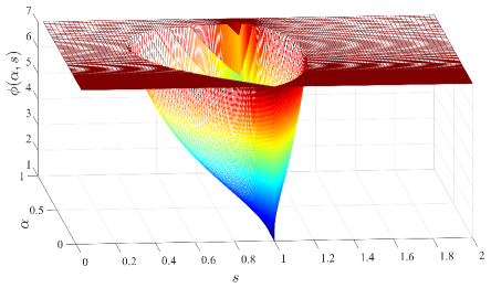
Figure 1: Local objective function $\phi$ of each agent as a function of its parameters. $s$ is the noise-to-state gain and $\alpha$ is related to the noise decaying ratio. We cap the function values at $7$ for visualization purposes. The function approaches its infimum as $\alpha\to 0$ while $s=1$.

Since $D$ is not compact, the infimum might not be attained, and in fact, this is the case. It is easy verify that $\lim_{\alpha\to 0}\phi(\alpha,1)=1$. Now, for all $(\alpha,s)\in D$, $1-(\alpha+(1-\alpha)\lvert s-1\rvert)^{2}<1$ so

$$\phi(\alpha,s)>\phi_{1}^{2}(\alpha,s),\;\phi_{1}(\alpha,s)=\frac{(\alpha+(1-\alpha)\lvert s-1\rvert)s}{\alpha(1-|s-1|)}.$$

If $s\leq 1$, then $\phi_{1}(\alpha,s)=s+\frac{1-s}{\alpha}>1$. If $s>1$, then $\phi_{1}(\alpha,s)>1+\frac{s-1}{\alpha(2-s)}>1$. Therefore, for all $(\alpha,s)\in D$, $\phi(\alpha,s)>1$, which completes the proof. ∎

Given that differential privacy is resilient to post-processing, an alternative design strategy to preserve the differential privacy of agents’ initial states is to inject noise only at the initial time, $k=0$. From (14), the introduction of a one-shot noise by agent $i$ corresponds to $q_{i}=0$ which is not feasible if $s_{i}\neq 1$. This can also be seen by rewriting (12) as

$$\theta(k+1)=(I-S)\theta(k)+(S-hL)x(k),$$

so if $s_{i}\neq 1$ for any $i$, $\theta_{i}(k)$ directly (not only through $x_{i}(0)$) depend on $\theta_{i}(0)$. However, if $s_{i}=1$, one can verify using a simplified version of the proof of Proposition 5.7 that $q_{i}=0$ also preserves $\epsilon_{i}$-differential privacy of $\theta_{i}(0)$ with $\epsilon_{i}=\frac{\delta}{c_{i}}$. This results in a cost of

$$J=\frac{2}{n^{2}}\sum_{i=1}^{n}c_{i}^{2}=\frac{2\delta^{2}}{n^{2}}\sum_{i=1}^{n}\frac{1}{\epsilon_{i}^{2}}=J^{*},$$

showing that the optimal accuracy is also achieved by one-shot perturbation of the initial state at time $k=0$ and injection of no noise thereafter. A similar conclusion (that one-shot Laplace perturbation minimizes the output entropy) can be drawn from (Wang et al., 2014), albeit this is not explicitly mentioned therein.

Remark 5.11.

(Dynamic Average Consensus) In dynamic average consensus (Bai et al., 2010; Zhu and Martínez, 2010; Kia et al., 2015), agents seek to compute the average of individual exogenous, time-varying signals (the “static” average consensus considered here would be a special case corresponding to the exogenous signals being constant). In such scenarios, it is straightforward to show, using an argument similar to Proposition 4.1, that one-shot perturbation would no longer preserve the differential privacy of time-varying input signals. The reason is that in this case, there is a recurrent flow of information at each node whose privacy can no longer be preserved with one-shot perturbation. Sequential perturbation as in (13)-(14) is then necessary and the variance of the noise sequence has to dynamically depend on the rate of information flow to each node. Although the detailed design of such algorithms is beyond the scope of this work, such an algorithm can be designed following the idea of the sequential perturbation design of this work and the proof of its privacy in Proposition 5.7. To see this, note that (for $S\neq I_{n}$) we “tune” the amount of noise injection $\eta_{i}(k)$ so that the privacy of $(1-s_{i})^{k}\theta_{0,i}$ is preserved at each round $k\geq 1$, but $(1-s_{i})^{k}\theta_{0,i}$ is the amount of “retained information” of $\theta_{0,i}$ at round $k$ and plays the same role as $u(k)$ in the dynamic average consensus problem. $\bullet$

6 Simulations

In this section, we report simulation results of the distributed dynamics (12)-(14) on a network of $n=50$ agents. Figure 2 shows the random graph used throughout the section, where edge weights are i.i.d. and each one equals a sum of two i.i.d. Bernoulli random variables with $p=0.1$. The agents’ initial states are also i.i.d. with distribution $\mathcal{N}(50,100)$. As can be seen from (24) and (25), neither accuracy nor privacy depend on the initial values or the communication topology (albeit according to (21) the convergence rate depends on the latter). In all the simulations, $\delta=1$ and $c_{i}=\delta q_{i}/\epsilon_{i}(q_{i}-|s_{i}-1|)$ for all $i\in\{1,\dots,n\}$.

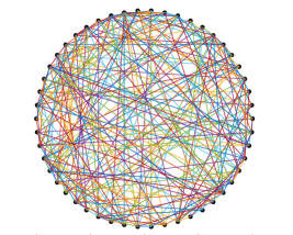
Figure 2: Random graph used for simulation.

Figure 3 depicts simulations with $\epsilon=0.1\cdot\mathbf{1}_{n}$ and $S=sI_{n}$ while sweeping $s$ over $[0.8,1.2]$ with logarithmic step size. For each value of $s$, we set $q_{i}=\alpha_{i}+(1-\alpha_{i})|s-1|$ with $\alpha_{i}=10^{-6}$ for each $i\in\{1,\dots,n\}$ and repeat the simulation $10^{4}$ times. For each run, to capture the statistical properties of the convergence point, the graph topology and initial conditions are the same and only noise realizations change. Figure 3(a) shows the empirical (sample) standard deviation of the convergence point as a function of $s$, verifying the optimality of one-shot perturbation. In particular, notice the sensitivity of the accuracy to $s$ close to $s=1$. Figure 3(b) shows the ‘settling time’, defined as the number of rounds until convergence (measured by a tolerance of $10^{-2}$), as a function of $s$. The fastest convergence is achieved for $s=1$, showing that one-shot noise is also optimal in the sense of convergence speed. We have observed the same trends as in Figure 3 for different random choices of initial conditions and network topologies. Note that the settling time depends on both the convergence rate and the initial distance from the convergence point $\|\theta(0)-\theta_{\infty}\mathbf{1}_{n}\|$. The former is constant at $\mu=\overline{\lambda}=0.84$ for $s\in[0.8,1.2]$. The latter depends on $\{c_{i}\}_{i=1}^{n}$, which in turn depend on $s$ by (32). This explains the trend observed in Figure 3(b).

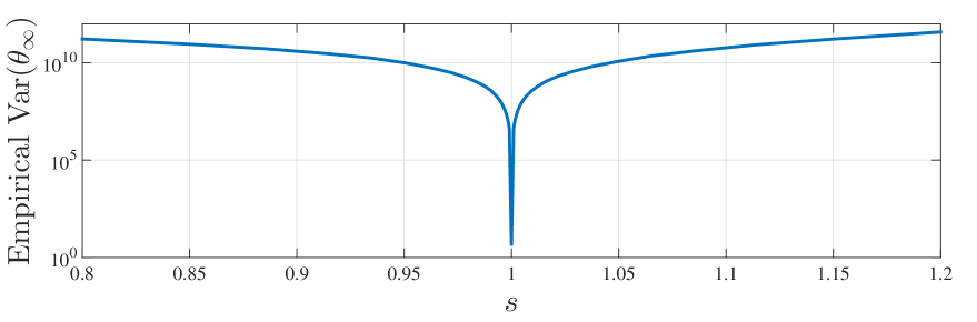
(a)

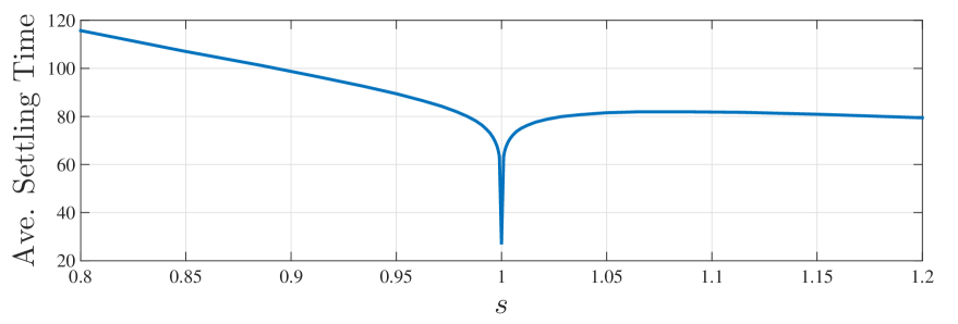
(b)

Figure 3: Executions of the algorithm (12)-(14) for random topology and initial conditions. (a) shows the empirical (i.e., sample) variance of the convergence point and (b) shows the settling time. The trend in (a) validates Proposition 5.10 while (b) shows the optimality of one-shot perturbation for convergence speed.

Figure 4 depicts the privacy-accuracy trade-off for the proposed algorithm. We have set $S=I_{n}$, $q=0\cdot\mathbf{1}_{n}$, and $\epsilon=\overline{\epsilon}\cdot\mathbf{1}_{n}$ and then swept $\overline{\epsilon}$ logarithmically over $[10^{-2},10^{2}]$. In Figure 4(a), the algorithm is run 25 times for each value of the $\overline{\epsilon}$ and the error $|\theta_{\infty}-\operatorname{Ave}(\theta_{0})|$ for each run is plotted as a circle. In Figure 4(b), the sample variance of the convergence point $\theta_{\infty}$ is shown as a function of $\overline{\epsilon}$ together with the theoretical value given in Proposition 5.10. In both plots, we see an inversely-proportional relationship between accuracy and privacy, as expected.

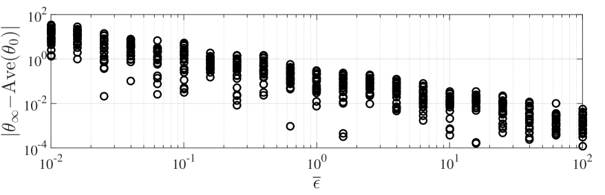
(a)

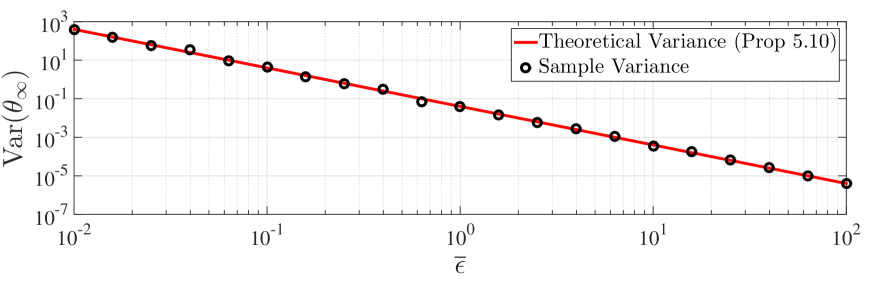
(b)

Figure 4: The privacy-accuracy trade-off for the proposed algorithm (12)-(14) for random topology and initial conditions. (a) shows the norm of the error for 25 different realizations of the noise and (b) shows the sample variance over 100 noise realizations as well as the theoretical value provided by Proposition 5.10. The trend in both figures conforms with the theoretical characterization of $\theta_{\infty}$ given in Corollary 5.5.

Figure 5 shows the histogram of convergence points for $10^{6}$ runs of the algorithm with $\epsilon=0.1\cdot\mathbf{1}_{n}$, $S=I_{n}$ and $q=0\cdot\mathbf{1}_{n}$ (optimal accuracy). The distribution of the convergence point is a bell-shaped curve with mean exactly at the true average, in accordance with Corollary 5.5.

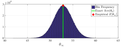
Figure 5: Statistical distribution of the convergence point. The sample mean (starred) matches the true average (green vertical line).

Although the distribution of $\theta_{\infty}$ is provably non-Gaussian, the central limit theorem, see e.g., (Durrett, 2010), implies that it is very close to Gaussian since the number of agents is large.

Finally, Figure 6 illustrates the convergence rate of the algorithm. Here, for $\epsilon=0.1\mathbf{1}_{n}$, $S=0.9I_{n}$, $q=0.2\mathbf{1}_{n}$, and the same topology as in the previous plots, the initial agents states are randomly selected and the whole algorithm is run 100 times with different noise realizations $\boldsymbol{\eta}$, each time until $100$ iterations. For each value of initial states and each $k\in\{1,\dots,100\}$, we empirically approximate the quantity

$$\left(\frac{\mathbb{E}\big{[}(\theta(k)-\theta_{\infty}\mathbf{1}_{n})^{T}(\theta(k)-\theta_{\infty}\mathbf{1}_{n})\big{]}}{\mathbb{E}\big{[}(\theta(0)-\theta_{\infty}\mathbf{1}_{n})^{T}(\theta(0)-\theta_{\infty}\mathbf{1}_{n})\big{]}}\right)^{1/2k}$$

by taking the sample mean instead of the expectation in the numerator and denominator. We repeat this whole process 50 times for different random initial conditions and plot the result, together with the theoretical value of $\mu$ (which in this case equals $\overline{\lambda}$) given by Proposition 5.4. As Figure 6 shows, the supremum of the resulting curves converges to $\mu$ as $k\to\infty$, as expected.

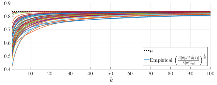
Figure 6: Illustration of the convergence rate of the algorithm (12)-(14). The limit of the supremum of the solid lines converges to the theoretical value of the exponential mean-square convergence rate $\mu$ given by Proposition 5.4. The curves with higher values correspond to initial states $\theta_{0}$ that are closer to the eigenvector of $I_{n}-hL-\Pi_{n}$ associated with $\overline{\lambda}$.

7 Conclusions

We have studied the problem of multi-agent average consensus subject to the differential privacy of agents’ initial states. We have showed that the requirement of differential privacy cannot be satisfied if agents’ states weakly converge to the exact average of their initial states. This result suggests that the most one can expect of a differentially private consensus algorithm is that the consensus value is unbiased, i.e., its expected value is the true average, and the variance is minimized. We have designed a linear consensus algorithm that meets this objective, and have carefully characterized its convergence, accuracy, and differential privacy properties. Future work will include the investigation of the limitations and advantages of differential privacy in multi-agent systems, the extension of the results to dynamic average consensus, distributed optimization, filtering, and estimation, and the design of algorithms for privacy preservation of the network structure and other parameters such as edge weights and vertex degrees.

References

- Bai et al. [2010] H. Bai, R. A. Freeman, and K. M. Lynch. Robust dynamic average consensus of time-varying inputs. In IEEE Conf. on Decision and Control, pages 3104–3109, Atlanta, GA, December 2010.
- Bullo et al. [2009] F. Bullo, J. Cortés, and S. Martínez. Distributed Control of Robotic Networks. Applied Mathematics Series. Princeton University Press, 2009. ISBN 978-0-691-14195-4. Electronically available at http://coordinationbook.info.
- Duan et al. [2015] X. Duan, J. He, P. Cheng, Y. Mo, and J. Chen. Privacy preserving maximum consensus. In IEEE Conf. on Decision and Control, pages 4517–4522, Osaka, 2015.
- Durrett [2010] R. Durrett. Probability: Theory and Examples. Series in Statistical and Probabilistic Mathematics. Cambridge University Press, 4th edition, 2010. ISBN 9780521765398.
- Dwork [2006] C. Dwork. Differential privacy. In Proceedings of the 33rd International Colloquium on Automata, Languages and Programming (ICALP), pages 1–12, Venice, Italy, July 2006.
- Dwork and Roth [2014] C. Dwork and A. Roth. The algorithmic foundations of differential privacy. Found. Trends Theor. Comput. Sci., 9(3-4):211–407, August 2014.
- Dwork et al. [2006] C. Dwork, F. McSherry, K. Nissim, and A. Smith. Calibrating noise to sensitivity in private data analysis. In Proceedings of the 3rd Theory of Cryptography Conference, pages 265–284, New York, NY, March 2006.
- Gündüz et al. [2010] D. Gündüz, E. Erkip, and H.V. Poor. Source coding under secrecy constraints. In Securing Wireless Communications at the Physical Layer, pages 173–199. Springer US, Boston, MA, 2010.
- Han et al. [2014] S. Han, U. Topcu, and G. J. Pappas. Differentially private convex optimization with piecewise affine objectives. In IEEE Conf. on Decision and Control, pages 2160–2166, Los Angeles, CA, December 2014.
- Huang et al. [2012] Z. Huang, S. Mitra, and G. Dullerud. Differentially private iterative synchronous consensus. In Proceedings of the 2012 ACM workshop on Privacy in the electronic society, pages 81–90, New York, NY, 2012.
- Huang et al. [2014] Z. Huang, Y. Wang, S. Mitra, and G. E. Dullerud. On the cost of differential privacy in distributed control systems. In Proceedings of the 3rd International Conference on High Confidence Networked Systems (HiCoNS), pages 105–114, Berlin, Germany, April 2014.
- Huang et al. [2015] Z. Huang, S. Mitra, and N. Vaidya. Differentially private distributed optimization. In Proceedings of the 2015 International Conference on Distributed Computing and Networking, Pilani, India, January 2015.
- Jiang and Wang [2001] Z.-P. Jiang and Y. Wang. Input-to-state stability for discrete-time nonlinear systems. Automatica, 37(6):857–869, 2001.
- Kairouz et al. [2015] P. Kairouz, S. Oh, and P. Viswanath. Secure multi-party differential privacy. In Advances in Neural Information Processing Systems 28, pages 2008–2016. Curran Associates, Inc., 2015.
- Kefayati et al. [2007] M. Kefayati, M. S. Talebi, B. H. Khalaj, and H. R. Rabiee. Secure consensus averaging in sensor networks using random offsets. In IEEE Intern. Conf. on Telec., and Malaysia Intern. Conf. on Communications, pages 556–560, Penang, May 2007.
- Kia et al. [2015] S. S. Kia, J. Cortés, and S. Martínez. Dynamic average consensus under limited control authority and privacy requirements. International Journal on Robust and Nonlinear Control, 25(13):1941–1966, 2015.
- Manitara and Hadjicostis [2013] N. E. Manitara and C. N. Hadjicostis. Privacy-preserving asymptotic average consensus. In European Control Conference, pages 760–765, Zurich, Switzerland, 2013.
- Mesbahi and Egerstedt [2010] M. Mesbahi and M. Egerstedt. Graph Theoretic Methods in Multiagent Networks. Applied Mathematics Series. Princeton University Press, 2010.
- Mo and Murray [2014] Y. Mo and R. M. Murray. Privacy preserving average consensus. In IEEE Conf. on Decision and Control, pages 2154–2159, Los Angeles, CA, December 2014.
- Mo and Murray [2015] Y. Mo and R. M. Murray. Privacy preserving average consensus. IEEE Transactions on Automatic Control, 2015. Submitted, available at http://yilinmo.github.io/public/papers/tac2014privacy.pdf.
- Mukherjee et al. [2014] A. Mukherjee, S.A.A. Fakoorian, J. Huang, and A.L. Swindlehurst. Principles of physical layer security in multiuser wireless networks: A survey. IEEE Communications Surveys & Tutorials, 16(3):1550–1573, 2014.
- Nozari et al. [2015] E. Nozari, P. Tallapragada, and J. Cortés. Differentially private average consensus with optimal noise selection. IFAC-PapersOnLine, 48(22):203–208, 2015. IFAC Workshop on Distributed Estimation and Control in Networked Systems, Philadelphia, PA.
- Nozari et al. [2017] E. Nozari, P. Tallapragada, and J. Cortés. Differentially private distributed convex optimization via functional perturbation. IEEE Transactions on Control of Network Systems, 2017. To appear.
- Ny and Pappas [2014] J. L. Ny and G. J. Pappas. Differentially private filtering. IEEE Transactions on Automatic Control, 59(2):341–354, 2014.
- Olfati-Saber et al. [2007] R. Olfati-Saber, J. A. Fax, and R. M. Murray. Consensus and cooperation in networked multi-agent systems. Proceedings of the IEEE, 95(1):215–233, 2007.
- Papoulis and Pillai [2002] A. Papoulis and S. U. Pillai, editors. Probability, Random Variables and Stochastic Processes. McGraw-Hill, 2002. ISBN 0073660116.
- Pettai and Laud [2015] M. Pettai and P. Laud. Combining differential privacy and secure multiparty computation. In Proceedings of the 31st Annual Computer Security Applications Conference, ACSAC 2015, pages 421–430. ACM, 2015.
- Ren and Beard [2008] W. Ren and R. W. Beard. Distributed Consensus in Multi-Vehicle Cooperative Control. Communications and Control Engineering. Springer, 2008. ISBN 978-1-84800-014-8.
- Tanaka and Sandberg [2015] T. Tanaka and H. Sandberg. SDP-based joint sensor and controller design for information-regularized optimal LQG control. In IEEE Conf. on Decision and Control, pages 4486–4491, Osaka, 2015.
- Wang et al. [2014] Y. Wang, Z. Huang, S. Mitra, and G. E. Dullerud. Entropy-minimizing mechanism for differential privacy of discrete-time linear feedback systems. In IEEE Conf. on Decision and Control, pages 2130–2135, Los Angeles, CA, December 2014.
- Zhu and Martínez [2010] M. Zhu and S. Martínez. Discrete-time dynamic average consensus. Automatica, 46(2):322–329, 2010.