Shock waves, rarefaction waves and non-equilibrium steady states
in quantum critical systems

Abstract

We re-examine the emergence of a universal non-equilibrium steady state following a local quench between quantum critical heat baths in spatial dimensions greater than one. We show that energy transport proceeds by the formation of an instantaneous shock wave and a broadening rarefaction wave on either side of the interface, and not by two shock waves as previously proposed. For small temperature differences the universal steady state energy currents of the two-shock and rarefaction-shock solutions coincide. Over a broad range of parameters, the difference in the energy flow across the interface between these two solutions is at the level of two percent. The properties of the energy flow remain fully universal and independent of the microscopic theory. We briefly discuss the width of the shock wave in a viscous fluid, the effects of momentum relaxation, and the generalization to charged fluids.

I Introduction

In recent years there has been intense experimental and theoretical activity exploring the behavior of non-equilibrium quantum systems Polkovnikov et al. (2011). Stimulated by experiment on low-dimensional cold atomic gases Kinoshita et al. (2006), theoretical work has focused on the dynamics of integrable models and their novel thermalization properties. An important finding is that integrable models are typically described by a Generalized Gibbs Ensemble (GGE) Rigol et al. (2007, 2008); Rigol (2009) due to the presence of an infinite number of conservation laws. However, there are very few theoretical results in non-integrable settings and in higher dimensions. Recent experiments on cold atomic gases Cao et al. (2011), Fermi liquids de Jong and Molenkamp (1995); D. A. Bandurin et al. ; Moll et al. , and charge neutral graphene J. Crossno et al. ; Lucas et al. , probe the dynamics of quantum systems in more than one dimension. It is timely to establish universal phenomena for such higher dimensional systems.

In recent work we investigated non-equilibrium energy transport between quantum critical heat baths in arbitrary dimensions Bhaseen et al. (2015), generalizing the results of Bernard and Doyon (2012) for one spatial dimension. We showed that a non-equilibrium steady state (NESS) emerges between the heat baths and that it is equivalent to a Lorentz boosted thermal state. The latter captures both the average energy current and its fluctuations. In particular, the energy current and its entire fluctuation spectrum is universally determined in terms of the effective “central charge” (the analogue of the Stefan-Boltzmann constant) of the quantum critical heat baths and their temperatures. A key observation is that the steady state is formed by propagating wavefronts emanating from the contact region. For small temperature differences these wavefronts are ordinary sound waves, but for large temperature differences their dynamics is non-linear. The properties of the NESS are constrained by the equation of state of the heat baths and the conservation of energy and momentum across the wavefronts. This hydrodynamic approach based on macroscopic conservation laws thus provides a valuable handle on non-equilibrium transport in arbitrary dimensions, establishing bridges between different fields of research. The emergence of a NESS bounded by two planar shock waves was also considered in Refs. Chang et al. (2014); Amado and Yarom (2015); Pourhasan .

In this paper we re-examine this problem of non-equilibrium energy flow in arbitrary dimensions. We show that the idealized solution in terms of two infinitely sharp shock waves requires modification in the light of thermodynamic and numerical considerations. In spatial dimensions $d>1$, one of the shocks is actually a smoothly varying and broadening rarefaction wave, even in the absence of viscosity. The results in $d=1$ are unaffected due to the light-cone propagation of the wavefronts, where the effective speed of light and the speed of sound coincide. In higher dimensions this is not the case and more complicated solutions may arise. Even in the presence of a broad rarefaction wave in $d>1$, we always find that a NESS is supported at the interface between the heat baths. This NESS can once again be understood as a Lorentz-boosted thermal state. In particular, numerical and analytical results for the solutions show that the steady state energy current is again universal. Quantitatively the effect of a broadening rarefaction wave is small: for the experimentally relevant dimensions of $d=2,3$, the results for the energy current across the interface agree to within about $2\%$ of the idealized sharp shock solution over a broad range of temperatures. In physically realizable systems, shock broadening will also occur due to viscous corrections  Bhaseen et al. (2015). We outline the non-perturbative effects of this broadening in Section III. We also provide a brief discussion of momentum relaxation in Section IV and of charged fluids in Section V. We conclude in Section VI with an outlook for future research.

II Universal NESS between quantum critical heat baths

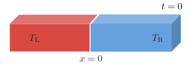
Figure 1: The set-up consists of two isolated quantum critical systems which are initially prepared at temperatures $T_{\mathrm{L}}$ and $T_{\mathrm{R}}$ and are instantaneously connected along a hyperplane at time $t=0$. A non-equilibrium steady state (NESS) forms at the interface between the heat baths carrying an average energy current $J_{\mathrm{E}}$. Within a hydrodynamic approach based on macroscopic conservation laws, the character of the NESS is determined by the equation of state of the heat baths and energy-momentum conservation across the resulting wavefronts. The latter may take the form of sharp shock waves or smoothly varying rarefaction waves, depending on the spatial dimensionality.

The set-up we consider is depicted in Fig. 1. Two infinitely large isolated but identical quantum critical systems are initially prepared at temperatures $T_{\mathrm{L}}$ and $T_{\mathrm{R}}$ and are brought into instantaneous contact along a hyperplane at time $t=0$ Bernard and Doyon (2012); Bhaseen et al. (2015). We restrict our attention to Lorentz invariant quantum critical points with an effective speed of light $v_{l}=1$. On connecting the two systems together, a NESS forms at the interface between the heat baths, carrying a ballistic energy current $J_{\mathrm{E}}=T^{tx}$, where $T^{\mu\nu}$ is the energy-momentum tensor. This “partitioning” setup may be regarded as a local quantum quench joining two independent sub-systems. Equivalently, we may consider applying an abrupt step temperature profile to an otherwise uniform system. In the context of hydrodynamics these initial conditions correspond to the so-called Riemann problem, to which we will return in Section II.1.

Let us briefly recall the results in $d=1$. In one spatial dimension a spatially homogeneous NESS is formed in the vicinity of the interface Bernard and Doyon (2012, 2013, 2015). The steady state carries a universal average energy current $J_{\mathrm{E}}=c\pi^{2}k_{\mathrm{B}}^{2}(T_{\mathrm{L}}^{2}-T_{\mathrm{R}}^{2})/6h$, where $c$ is the central charge of the heat baths. This may be regarded as an application of the Stefan-Boltzmann law to quantum critical systems, where the internal energy density is proportional to $T^{d+1}$ Cardy (2010). The result for $J_{\mathrm{E}}$ extends earlier results for free fermions and bosons Pendry (1983); Sivan and Imry (1986); Butcher (1990); Fazio et al. (1998), as confirmed by transport experiments on ballistic channels Jezouin et al. (2013); Schwab et al. (2000); Rego and Kirczenow (1998). The generalization to arbitrary $c$ has been verified by time-dependent Density Matrix Renormalization Group (DMRG) methods on quantum spin chains Karrasch et al. (2013, 2012, 2013); Huang et al. (2013). Moreover, the exact generating function of energy current fluctuations has also been determined Bernard and Doyon (2012, 2013, 2015).

In Ref. Bhaseen et al. (2015) we discussed this non-equilibrium energy transport problem from a rather different vantage point. By combining insights from gauge-gravity duality and the dynamics of energy and momentum conservation, we showed that the 1+1 dimensional NESS is completely equivalent to a Lorentz boosted thermal state: by “running” past a thermal state at temperature $T=\sqrt{T_{\mathrm{L}}T_{\mathrm{R}}}$ it is possible to reproduce both the average energy flow and the full spectrum of energy current fluctuations in the NESS. Moreover, it is possible to extract the time-dependence from the solution of the macroscopic conservation laws $\partial_{\mu}T^{\mu\nu}=0$ in $1+1$ dimensions. The spatially homogeneous region is formed by outgoing “shock waves” which emanate from the point of contact at the effective speed of light; see Fig. 2.

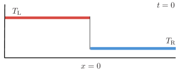
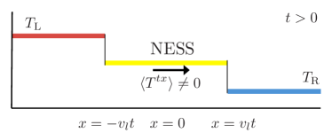
Figure 2: In one spatial dimension a spatially homogeneous steady state region is formed by outgoing shock waves moving at the effective speed of light $v_{l}$. The energy current $J_{\mathrm{E}}$ and the exact spectrum of energy current fluctuations are completely described a Lorentz boosted thermal state with temperature $T=\sqrt{T_{\mathrm{L}}T_{\mathrm{R}}}$.

In particular, the form of the steady state solution is uniquely determined by energy-momentum conservation across the shock fronts. This macroscopic conservation law approach is readily generalized to other equations of state for the energy baths. This has been recently demonstrated for perturbed 1+1 dimensional CFTs Bernard and Doyon . The use of conservation laws across large transition regions has also led to a thermodynamic description for the total, integrated current in one-dimensional systems Vasseur et al. . This growing body of work opens the door to wider applications of hydrodynamic techniques in low-dimensional quantum systems; for earlier work in this direction see for example Ref. Abanov and Wiegmann (2005).

II.1 The NESS in $d>1$

In Ref. Bhaseen et al. (2015) we argued that the above results could be generalized to higher dimensions by invoking the techniques of relativistic hydrodynamics. In particular, we showed that the numerical solution of conformal hydrodynamics leads to a non-trivial NESS in $d=2$, that is robust to a variety of perturbations. Moreover, we showed that both the average energy current $J_{\rm E}$ and the shock speeds $u_{\rm L,R}$, were in very good quantitative agreement with analytical solutions based on idealized two-shock solutions; see Fig 3(a). In this work we re-visit this two-shock ansatz, which we stressed in Ref. Bhaseen et al. (2015) is not a unique solution, and show that it is necessary to include rarefaction waves based on thermodynamic arguments; see Fig 3(b). We show that this leads to even better agreement with our numerical simulations. Importantly, the solution still contains a NESS, and the properties of this NESS can be determined analytically, though there is a change in the exact results compared to the idealized two-shock solution. The solution is still universal, and is solely determined by $T_{\mathrm{L,R}}$ and the analogue of the central charge of the quantum critical theories.

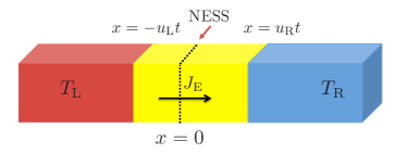
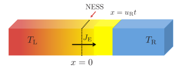
Figure 3: (a) Idealized solutions to conformal hydrodynamics in $d>1$ consisting of two planar shock waves emanating from the contact region. Thermodynamic consistency requires that the left-moving shock wave is replaced by a smooth rarefaction wave, even in the absence of viscosity. (b) Modified solution consisting of a left-moving rarefaction wave and a right-moving shock wave. The difference between the average energy current $J_{\rm E}$ across the interface in the two cases is about two percent. Note that a spatially homogeneous region also occurs to the right of the rarefaction wave as indicated by the solid yellow shading; see Fig. 4.

II.2 Hydrodynamic Limit

As for any interacting theory, with strongly coupled conformal field theories (CFTs) describing the quantum critical heat baths in Fig. 1, the late-time behavior following the local quench is expected to be captured by relativistic hydrodynamics. In particular, for a strongly coupled fluid at temperature $T$, we expect that hydrodynamics provides a good description of the non-equilibrium dynamics of conserved quantities on time scales long compared to $1/T$. As the relevant time scale $t\rightarrow\infty$, higher derivative corrections to the hydrodynamic equations can be neglected Bhaseen et al. (2015). Thus the relevant hydrodynamic equations are the conservation of energy and momentum:

$$\partial_{\mu}T^{\mu\nu}=0.$$ (1)

For a quantum critical state in local equilibrium, we know that

$$T^{\mu\nu}=CT^{d+1}\left[(d+1)u^{\mu}u^{\nu}+\eta^{\mu\nu}\right].$$ (2)

Here $\eta^{\mu\nu}={\rm diag}(-1,1,\dots,1)$ is the Minkowski space-time metric and $u^{\mu}$ is the local fluid velocity. This formula is valid both in the asymptotic baths, and in the emergent NESS. The only non-universal part of $T^{\mu\nu}$ is the constant $C$, which effectively counts the number of degrees of freedom in the CFT; it can be considered as a generalization of the central charge of $d=1$ dimensional theories. Bringing two hydrodynamical systems with $T=T_{\mathrm{L}}$ for $x<0$ and $T=T_{\mathrm{R}}$ for $x>0$ into contact along a local interface is known as the Riemann problem in fluid dynamics. We will consider the solutions to this problem below.

II.3 Two-Shock Solution

The solutions of perfect conformal hydrodynamics are not unique for $d>1$, in contrast to $d=1$. Hence, to find a proper solution to the Riemann problem requires additional physical input. Guided by the exact shock wave solutions found in $d=1$, we suggested that a NESS would arise between planar shock waves in $d>1$. Using this ansatz we argued previously Bhaseen et al. (2015) that the non-equilibrium steady state was equivalent to a Lorentz boosted thermal state at temperature

$$T_{\mathrm{s}}=\sqrt{T_{\mathrm{L}}T_{\mathrm{R}}}.$$ (3)

The corresponding energy flow was given by Bhaseen et al. (2015)

$$J_{\mathrm{E}}\equiv T^{tx}_{\mathrm{s}}=C\frac{T_{\mathrm{L}}^{d+1}-T_{\mathrm{R}}^{d+1}}{v_{\mathrm{R}}+(dv_{\mathrm{R}})^{-1}},\;\;\;\;\;v_{\mathrm{R}}=\sqrt{\frac{1}{d}\frac{dT_{\mathrm{L}}^{(d+1)/2}+T_{\mathrm{R}}^{(d+1)/2}}{dT_{\mathrm{R}}^{(d+1)/2}+T_{\mathrm{L}}^{(d+1)/2}}}.$$ (4)

In particular, this NESS was separated by two asymmetrically moving shock waves, that can be identified as non-linear sound waves; see Fig. 3(a). Checking this ansatz against numerical simulations of conformal hydrodynamics we found very good agreement with our analytical prediction for $J_{\mathrm{E}}$, even far from the linear response regime.

In spite of this agreement, this solution is problematic for the following physical reason. If we truncate the hydrodynamic gradient expansion at zeroth order in derivatives (perfect hydrodynamics), then Eq. (1) implies conservation of entropy

$$\partial_{\mu}\left((d+1)CT^{d}u^{\mu}\right)\equiv\partial_{\mu}s^{\mu}=0,$$ (5)

on any smooth solution. However, at an infinitely sharp shock wave this criterion is generally violated. This is not a problem, as long as $\partial_{\mu}s^{\mu}\geq 0$, which is a local statement of the second law of thermodynamics. This is a constraint of hydrodynamics at all orders in the gradient expansion. At first order for a conformal fluid, we have $\partial_{\mu}s^{\mu}\sim\eta(\partial v)^{2}/T$ (schematically). The fact that viscosity is required to create entropy at a shock front is a subtlety we will return to in the next section. Away from these shock fronts, we will have $\partial_{\mu}s^{\mu}=0$ in perfect fluid dynamics.

Consider now a shock wave moving at velocity $v_{\mathrm{shock}}$, with $T_{<}$ and $v_{<}$ the fluid temperature and velocity to the left of the shock, and $T_{>}$ and $v_{>}$ the fluid temperature and velocity to the right of the shock. Then, integrating over a shock of transverse area $A$ across a time step $t$, we find that

$$\int\limits_{\text{shock}}\mathrm{d}t\mathrm{d}^{d}\mathbf{x}\;\partial_{\mu}\left((d+1)CT^{d}u^{\mu}\right)=At\times(d+1)C\left[\frac{T_{>}^{d}(v_{>}-v_{\mathrm{shock}})}{\sqrt{1-v_{>}^{2}}}-\frac{T_{<}^{d}(v_{<}-v_{\mathrm{shock}})}{\sqrt{1-v_{<}^{2}}}\right].$$ (6)

By the argument above, on a physical solution, the right hand side must be positive. However, one can show that for the shock moving into the region of higher temperature in this two-shock solution (the left-moving one), the entropy production given by Eq. (6) is negative. We now describe the modification of this shock wave so that there is no local entropy loss.

II.4 Rarefaction Waves

Because only the left-moving shock violates the second law of thermodynamics, we will look for a different solution to the Riemann problem where the left-moving shock is replaced with a left-moving rarefaction wave; see Fig. 3(b). This is a solution that is continuous, but whose first derivatives are discontinuous Taub (1948); Thompson (1986); Lax (1957); Liu (1975); Marti and Müller (2003), and where $T$ and $v\equiv u^{x}/u^{t}$ are functions of $x/t\equiv\xi$ alone. By assumption therefore the local configuration is always in local equilibrium, in contrast to a true shock. Very similar solutions were presented in Mach and Pietka (2010). The non-trivial equations of hydrodynamics are the $t$ and $x$ components of (1), and may be expressed as ordinary differential equations in $\xi$:

$$\xi\frac{\mathrm{d}}{\mathrm{d}\xi}\left(T^{d+1}\frac{d+v^{2}}{1-v^{2}}\right) =\frac{\mathrm{d}}{\mathrm{d}\xi}\left(T^{d+1}\frac{(d+1)v}{1-v^{2}}\right),$$ (7a)

$$\xi\frac{\mathrm{d}}{\mathrm{d}\xi}\left(T^{d+1}\frac{(d+1)v}{1-v^{2}}\right) =\frac{\mathrm{d}}{\mathrm{d}\xi}\left(T^{d+1}\frac{1+dv^{2}}{1-v^{2}}\right).$$ (7b)

Note that the coefficient $C$ of the local equilibrium configuration drops out, and the solution for the rarefaction profile is independent of the value of this parameter.

As in Mach and Pietka (2010), this pair of equations can be re-organized into the form

$$\left(\begin{array}[]{c}0\\ 0\end{array}\right)=\mathsf{M}(\xi)\left(\begin{array}[]{c}\mathrm{d}T/\mathrm{d}\xi\\ \mathrm{d}v/\mathrm{d}\xi\end{array}\right),$$ (8)

and is thus only satisfied when $\det(\mathsf{M}(\xi))=0$. A straightforward calculation reveals that this occurs when

$$\left((d+1)v-\left(d+v^{2}\right)\xi\right)\left(2v-\left(1+v^{2}\right)\xi\right)=\left(1+v^{2}-2v\xi\right)\left(1+dv^{2}-(d+1)v\xi\right).$$ (9)

After further algebraic manipulations, we find that this occurs when

$$\xi=\frac{v\pm c_{\mathrm{s}}}{1\pm c_{\mathrm{s}}v},$$ (10)

where

$$c_{\mathrm{s}}=\frac{1}{\sqrt{d}}$$ (11)

is the speed of sound in a scale invariant quantum critical fluid. Eq. (10) is the relativistic velocity addition law between $\pm c_{\mathrm{s}}$ and the local fluid velocity in the $x$-direction, $v$. A straightforward inversion reveals that

$$v=\frac{\xi\mp c_{\mathrm{s}}}{1\mp c_{\mathrm{s}}\xi}.$$ (12)

As this left-moving rarefaction wave should begin ($v=0$) when $\xi<0$, we conclude that we must take the minus sign in Eq. (10) and the plus sign in Eq. (12). Next, we employ entropy conservation in the rarefaction wave, and obtain

$$\xi\frac{\mathrm{d}}{\mathrm{d}\xi}\left(\frac{T^{d}}{\sqrt{1-v^{2}}}\right)=\frac{\mathrm{d}}{\mathrm{d}\xi}\left(\frac{T^{d}v}{\sqrt{1-v^{2}}}\right).$$ (13)

Using the relation between $v$ and $\xi$ in a left-moving rarefaction wave, we convert this equation into a differential equation for $\mathrm{d}T/\mathrm{d}v$, which may be solved exactly. Employing the boundary conditions $T=T_{\rm L}$ at the left-edge of the rarefaction wave gives

$$T=T_{\mathrm{L}}\left(\frac{1-v}{1+v}\right)^{1/2\sqrt{d}}.$$ (14)

Let us now describe the rarefaction wave. For $\xi<-c_{\mathrm{s}}$, the solution is $T=T_{\mathrm{L}}$ and $v=0$. For $-c_{\mathrm{s}}<\xi<\xi^{*}$, the solution is described by the relations (14) and (10). For $\xi^{*}<\xi<u_{\mathrm{R}}$, the solution is given by a homogeneous region at temperature $T_{\mathrm{h}}$ and boosted by a velocity $v_{\mathrm{h}}$. Eq. (14) implies that these are related via

$$T_{\mathrm{h}}=T_{\mathrm{L}}\left(\frac{1-v_{\mathrm{h}}}{1+v_{\mathrm{h}}}\right)^{1/2\sqrt{d}}.$$ (15)

At $\xi=u_{\mathrm{R}}$ there is a shock wave, and for $\xi>u_{\mathrm{R}}$, the temperature is $T_{\mathrm{R}}$ and $v=0$.

The complete solution still has the undetermined parameters: $\xi^{*}$, $u_{\mathrm{R}}$, $T_{\mathrm{h}}$ and $v_{\mathrm{h}}$. We can fix these as follows. Eq. (10) determines $\xi^{*}$ from $v_{\mathrm{h}}$. We then employ the Rankine-Hugoniot conditions (corresponding to energy and momentum conservation) at the right-moving shock wave to obtain

$$\frac{(d+1)T_{\mathrm{h}}^{d+1}v_{\mathrm{h}}}{1-v_{\mathrm{h}}^{2}}-u_{\mathrm{R}}T_{\mathrm{h}}^{d+1}\frac{d+v_{\mathrm{h}}^{2}}{1-v_{\mathrm{h}}^{2}} =-du_{\mathrm{R}}T_{\mathrm{R}}^{d+1},$$ (16a)

$$\frac{1+dv_{\mathrm{h}}^{2}}{1-v_{\mathrm{h}}^{2}}T_{\mathrm{h}}^{d+1}-\frac{(d+1)v_{\mathrm{h}}}{1-v_{\mathrm{h}}^{2}}u_{\mathrm{R}}T_{\mathrm{h}}^{d+1} =T_{\mathrm{R}}^{d+1}.$$ (16b)

These equations fix a relation between $T_{\mathrm{h}}$ and $v_{\mathrm{h}}$:

$$T_{\mathrm{h}}=T_{\mathrm{R}}\left[\frac{2d+\left(1+d^{2}\right)v_{\mathrm{h}}^{2}+(d+1)v_{\mathrm{h}}\sqrt{4d+(d-1)^{2}v_{\mathrm{h}}^{2}}}{2d\left(1-v^{2}_{\mathrm{h}}\right)}\right]^{1/(d+1)}.$$ (17)

At this point, $u_{\mathrm{R}}$ is also fixed in terms of $v_{\mathrm{h}}$ and $T_{\mathrm{h}}$. We now have two formulas, Eqs. (15) and (17) for $T_{\mathrm{h}}$. There is a unique value of $v_{\mathrm{h}}$ which satisfies both, and this completely fixes our solution. We provide a qualitative sketch of the final temperature profile $T(\xi)$ for two different temperature ratios $T_{\mathrm{L}}/T_{\mathrm{R}}$ in Fig. 4, clarifying the role of the parameters defined above. For an observer at a fixed position $x$, at late times ($t\rightarrow\infty$) $\xi\rightarrow 0$. As we will see, the energy current is generically non-vanishing, and this defines a NESS, which is centered at $x=0$.

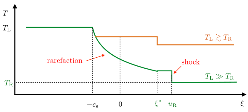
Figure 4: A qualitative sketch of the temperature profile $T(\xi)$ in the rarefaction-shock solution to the Riemann problem with heat baths at temperatures $T_{\mathrm{L}}$ and $T_{\mathrm{R}}$. The curves correspond to different values of $T_{\mathrm{R}}$ (for fixed $T_{\mathrm{L}}$) with $T_{\mathrm{L}}\gtrsim T_{\mathrm{R}}$ (orange) and $T_{\mathrm{L}}\gg T_{\mathrm{R}}$ (green). The profiles coincide up until the homogeneous region in between the rarefaction and the shock. The location of the latter is dependent on $T_{\mathrm{R}}$. For $T_{\mathrm{L}}/T_{\mathrm{R}}<\Gamma$ as given by Eq. (21), a spatially homogeneous profile envelops the contact interface (orange), while for $T_{\mathrm{L}}/T_{\mathrm{R}}>\Gamma$ the interface resides in the rarefaction region (green). A steady state energy current $J_{\mathrm{E}}$ is established at the interface in both cases.

As may be seen from Fig. 4, it is possible for the rarefaction wave to envelop the contact interface at $x=0$. Employing Eq. (10) we see that this occurs when the local speed in the homogeneous region as measured in the laboratory rest frame exceeds the speed of sound:

$$v_{\mathrm{h}}>c_{s}=\frac{1}{\sqrt{d}}.$$ (18)

This occurs at a critical temperature ratio

$$\frac{T_{\mathrm{L}}}{T_{\mathrm{R}}} =\Gamma\equiv\left(\frac{\sqrt{d}+1}{\sqrt{d}-1}\right)^{1/2\sqrt{d}}\left(\frac{3d+d^{-1}+(d+1)\sqrt{4+(d-1)^{2}d^{-3/2}}}{2(d-1)}\right)^{1/(d+1)}$$

$$\approx\left\{\begin{array}[]{ll}3.459&\ d=2\\ 2.132&\ d=3\end{array}\right..$$ (21)

When $T_{\mathrm{L}}/T_{\mathrm{R}}<\Gamma$, the rarefaction wave does not include the origin, and so the NESS is spatially homogeneous about $x=0$ at finite time $t$. When $T_{\mathrm{L}}/T_{\mathrm{R}}>\Gamma$, the NESS is contained in the rarefaction wave, and only becomes spatially homogeneous asymptotically as $t\rightarrow\infty$; see Fig. 4.

It is interesting that the equations derived above for a rarefaction wave coincide with the exact (two-shock) results in $d=1$ Bernard and Doyon (2012); Bhaseen et al. (2015). However, we stress that there is no rarefaction wave in $d=1$.

II.5 Energy Transport at the Interface

Having established the rarefaction-shock solution, we now examine the energy current at the interface $x=0$, the location of the emergent NESS. The energy current at the interface $J_{\mathrm{E}}=T^{tx}$ follows by computing $T(\xi=0)\equiv T_{0}$ and $v(\xi=0)\equiv v_{0}$, and employing Eq. (2):

$$J_{\mathrm{E}}=(d+1)CT_{0}^{d+1}\frac{v_{0}}{1-v_{0}^{2}}.$$ (22)

Consider first the limit where $T_{\mathrm{L}}\approx T_{\mathrm{R}}$. In this regime, the rarefaction wave does not envelop the origin. We find $T_{0}\approx(T_{\mathrm{L}}+T_{\mathrm{R}})/2$ and (see Appendix A)

$$J_{\mathrm{E}}\approx\frac{C\sqrt{d}(d+1)}{2}\left(\frac{T_{\mathrm{L}}+T_{\mathrm{R}}}{2}\right)^{d}(T_{\mathrm{L}}-T_{\mathrm{R}}).$$ (23)

The rarefaction-shock and two-shock solutions both reproduce this result, at leading order in $T_{\mathrm{L}}-T_{\mathrm{R}}$. When $T_{\mathrm{L}}/T_{\mathrm{R}}>\Gamma$, the rarefaction wave envelops the origin and we find a universal result

$$J_{\mathrm{E}}=C\frac{(d+1)\sqrt{d}}{d-1}\left(\frac{\sqrt{d}-1}{\sqrt{d}+1}\right)^{(d+1)/2\sqrt{d}}T_{\mathrm{L}}^{d+1}.$$ (24)

Surprisingly, Eq. (24) is independent of $T_{\mathrm{R}}$.

More generally, we can numerically solve (15) and (17) to compute $J_{\mathrm{E}}$ at any $T_{\mathrm{L},\mathrm{R}}$. Notably, the rarefaction-shock result for $J_{\mathrm{E}}$ is very close to the one predicted using the two-shock solution, even as $T_{\mathrm{L}}/T_{\mathrm{R}}\rightarrow\infty$. The two predictions are within $2\%$ of each other in the $T_{\mathrm{L}}/T_{\mathrm{R}}\rightarrow\infty$ limit in both $d=2$ and $d=3$; see Fig. 5.

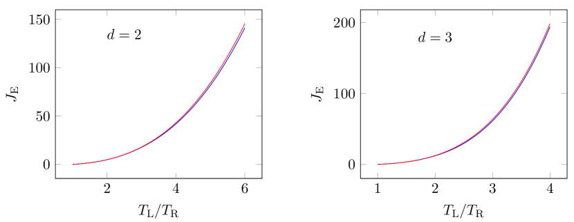
Figure 5: A comparison of the rarefaction-shock prediction for $J_{\mathrm{E}}=T^{tx}(x=0)$ (blue), compared to the two-shock prediction (red), in $d=2,3$. It is readily seen that results are numerically very close to each other. For simplicity, we have measured $J_{\mathrm{E}}$ in units of $CT_{\mathrm{R}}^{d+1}$ in the above plots.

The difference between the rarefaction-shock and two-shock solutions is most transparent in the spatial profile of physical observables. This is clearly seen in Fig. 6 which compares the $x$ and $t$ dependence of the rarefaction-shock and two-shock solutions, to the numerical solution of perfect conformal hydrodynamics given in Ref. Bhaseen et al. (2015). Note that at the rather extreme pressure ratio of $P_{\mathrm{L}}/P_{\mathrm{R}}>100$ (where $P=CT^{d+1}$ in the fluid rest frame), where the rarefaction wave envelops the origin, finite size effects are present in our numerical results.

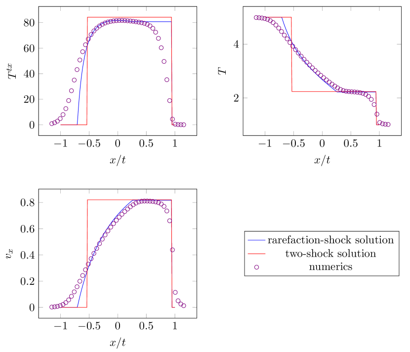
Figure 6: A comparison of the hydrodynamic variables $T(x,t)$, $v(x,t)$ and the resulting energy current, $T^{tx}(t,x)$ in the rarefaction-shock solution versus the two-shock solution. We have also included the numerical solution of Bhaseen et al. (2015) of the Riemann problem (with a smoothed temperature profile) in $d=2$, with $T_{\mathrm{L}}=5$ and $T_{\mathrm{R}}=C=1$. The numerical data are taken at time $t=1.25$, with initial conditions $T(x,t=0)=(T_{\mathrm{L}}+T_{\mathrm{R}})/2-(T_{\mathrm{L}}-T_{\mathrm{R}})\tanh(6.5\sin(x))$, with periodic boundary conditions at $x=\pm\pi$. It is readily seen that the rarefaction-shock solution provides a better fit to the data than the two-shock solution.

III Viscous Corrections

In this section we clarify the qualitative role of dissipative viscous corrections to the rarefaction-shock dynamics above, and describe the width of the right-moving shock wave when $T_{\mathrm{L}}>T_{\mathrm{R}}$. We focus on $T_{\mathrm{L}}-T_{\mathrm{R}}\ll T_{\mathrm{R}}$ for simplicity. Perturbatively, we showed Bhaseen et al. (2015) at intermediate time scales that the shock width will grow diffusively: $l_{\mathrm{shock}}\sim\sqrt{Dt}$ with diffusion constant $D\sim\eta T^{-d-1}$ and viscosity $\eta$. Our purpose in this section is to expand on this result, and to argue that perturbation theory fails at late times.

We know from Eq. (6) that the entropy production at the shock front, per unit transverse area per unit time, is given by

$$\mathcal{S}=(d+1)C\left[\frac{T_{\mathrm{h}}^{d}(u_{{\mathrm{R}}}-v_{\mathrm{h}})}{\sqrt{1-v_{\mathrm{h}}^{2}}}-T_{\mathrm{R}}^{d}u_{\mathrm{R}}\right].$$ (25)

In terms of $\delta\equiv T_{\mathrm{L}}/T_{\mathrm{R}}-1$, we find (using results from Appendix A):

$$\mathcal{S}=\frac{\sqrt{d}\left(d^{2}-1\right)}{48}CT_{\mathrm{R}}^{d}\delta^{3}+\mathrm{O}\left(\delta^{4}\right).$$ (26)

As in the non-relativistic case Landau and Lifshitz (1987), $\mathcal{S}$ vanishes at leading order in $\delta$, and only appears at order $\delta^{3}$. We can relate $\mathcal{S}$ to the width of the shock by noting that in a conformal fluid, the only source of entropy production (at leading order) is through viscous dissipation, so a scaling argument immediately leads to

$${\mathcal{S}}_{\text{p}ert}\sim\int\limits_{\mathrm{shock}}\mathrm{d}x\;\frac{\eta}{T}\left(\partial_{x}v_{x}\right)^{2}.$$ (27)

Evaluating this on the perturbative solution corresponding to a gaussian profile with width $l_{\text{s}hock}\sim\sqrt{Dt}$ one obtains

$${\mathcal{S}}_{\text{p}ert}\sim\frac{\eta v_{\mathrm{h}}^{2}}{Tl_{\mathrm{shock}}}.$$ (28)

At late times this entropy production rate is not sufficient to be compatible with Eq. (26). We conclude that perturbation theory breaks down at a characteristic timescale

$$t_{\mathrm{shock}}\sim\frac{\eta}{T_{\mathrm{R}}^{d+1}\delta^{2}},$$ (29)

making it clear that this effect is non-perturbative in $\delta$. This effect cannot be seen by directly solving the hydrodynamic equations perturbatively with the step (Riemann) profile. In non-relativistic fluids, it is typically the case that the shock simply stops growing, and maintains a finite width, similar to a soliton Landau and Lifshitz (1987). It would be interesting to confirm this for the relativistic fluid.

In the regime where $T_{\mathrm{L}}\gg T_{\mathrm{R}}$, the above argument breaks down. Noting by dimensional analysis that $\eta\sim T^{d}$, we estimate that perturbation theory breaks down when

$$l_{\mathrm{shock}}\sim\frac{1}{T_{\mathrm{L}}}.$$ (30)

It would be interesting to study this problem more carefully in future work, most likely through numerical simulations. Since our estimate of $l_{\mathrm{shock}}$ is comparable to the scale at which hydrodynamics itself breaks down, higher derivative corrections to the hydrodynamic equations cannot be neglected. This work could potentially be carried out using gauge-gravity duality, as this holographic approach automatically “resums” hydrodynamics to all orders in the gradient expansion.

IV Momentum Relaxation

In the previous sections, we have focused on fluids without impurities or other lattice effects which break translation invariance. In many realistic physical systems (such as electron fluids in metals), these effects are present, but if weak, they may be systematically accounted for within a hydrodynamic framework. As these effects violate momentum conservation, we may extend the hydrodynamic equations (1) on very long wavelengths to:

$$\partial_{\mu}T^{\mu t} =0,$$ (31a)

$$\partial_{\mu}T^{\mu i} =-\frac{T^{ti}}{\tau}.$$ (31b)

Here, $\tau$ is a phenomenological parameter corresponding to the time scale over which momentum decays. The validity of this hydrodynamic approximation has been shown explicitly in the limit where the fluid velocity is small compared to the speed of light by coupling the fluid to sources which break translational symmetry Lucas (2015). However, Eq. (31) has been used for quite some time (see e.g. Hartnoll et al. (2007); Davison (2013); Blake (2015)). When the rate is small and momentum relaxation is weak, the stress tensor of the fluid will be approximately unchanged from the clean fluid Lucas (2015), and we may continue to use the stress tensor (2). The validity of (31) for flow velocities comparable to the speed of light is less clear, but as we’ll see, the fluid velocities tend to be small at late times. We therefore expect that our discussion is qualitatively right.

As we discussed earlier for the Riemann problem, the temperatures in the problem do not introduce a relevant time scale for hydrodynamic phenomena. At the perfect fluid level, the only time scale in the problem is $\tau$. For $t\ll\tau$, the dynamics of the fluid is effectively described by the solution of Section II.4. For $t\gg\tau$, if the system reaches a steady state where $\partial_{t}$ and $\partial_{x}$ are “small”, the energy flow is determined by the equation

$$T^{tx}\approx-\tau\partial_{x}T^{xx}.$$ (32)

Hence, if a steady state forms, the fluid velocity and $T^{tx}$ vanish as $t\rightarrow\infty$, yielding an equilibrium state with

$$T^{tt}\approx dT^{xx}.$$ (33)

Hence, the momentum-relaxing hydrodynamic equations lead to a diffusion equation for the energy density $\epsilon=T^{tt}=dCT^{d+1}$ (and pressure) for $t\gg\tau$:

$$\partial_{t}\epsilon\approx\frac{\tau}{d}\partial_{x}^{2}\epsilon,$$ (34)

where the diffusion constant is $\tau c_{\mathrm{s}}^{2}$; since this is perfect conformal hydrodynamics, the speed of sound is $c_{\mathrm{s}}^{2}=1/d$. Remarkably, although the dynamics for $t\ll\tau$ is highly nonlinear, momentum relaxation reduces the late time dynamics to simple diffusion. We conclude that when $t\gg\tau$:

$$\epsilon=dC\left[\frac{T_{\mathrm{R}}^{d+1}+T_{\mathrm{L}}^{d+1}}{2}+\frac{T_{\mathrm{R}}^{d+1}-T_{\mathrm{L}}^{d+1}}{2}\mathrm{erf}\frac{x}{\sqrt{t\tau/d}}\right].$$ (35)

This late time behavior can also be seen by considering the fate of sound modes in the linear response regime Davison (2013). Fig. 7 shows a numerical simulation of the equations of momentum relaxing hydrodynamics. It is clear that the NESS does not persist for times $t\gtrsim\tau$.

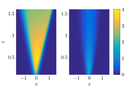
Figure 7: An intensity plot of $T^{tx}$ as a function of $x$ and $t$, in conformal hydrodynamics with momentum relaxation. We use the same initial conditions as in Fig. 6, but with $T_{\mathrm{L}}=2$. The left panel shows $\tau=3$, and the right panel shows $\tau=0.3$. The value of the energy current, and the width of the region between the shock waves, is evidently reduced in the right panel.

Indeed, as $t\rightarrow\infty$, $T^{tx}\sim t^{-1/2}$, as is readily shown from Eqs (32), (33) and (35). We have confirmed this numerically in Fig. 8. Experimental observation of the NESS thus requires probing the quantum dynamics of these inhomogeneous systems on fast time scales compared to $\tau$.

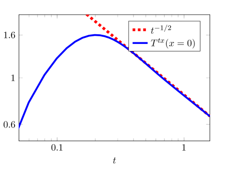
Figure 8: The algebraic decay of the energy current at the interface obtained by conformal hydrodynamics with momentum relaxation. We use the same initial conditions as in Fig. 7 and set $\tau=0.3$.

V Charged Fluids

A straightforward extension of our results in $d>1$ is to quantum critical systems with a conserved charge. In that case, the two asymptotic heat baths may have different chemical potentials $\mu_{\mathrm{L,R}}$, in addition to different temperatures $T_{\mathrm{L,R}}$. Eq. (1) is then supplemented by charge conservation,

$$\partial_{\mu}J^{\mu}=0.$$ (36)

For a perfect fluid,

$$J^{\mu}=nu^{\mu},$$ (37)

where $n$ is the charge density. In a relativistic gapless fluid, Eq. (2) is unchanged (see e.g. Lucas et al. ), up to replacing $CT^{d+1}$ with $P(\mu,T)$, the pressure in the local fluid rest frame. Hence, the dynamics of $P$ and $u^{\mu}$ closes and decouples from the dynamics of $n$. The energy-momentum dynamics is therefore the same as described in Section II.4, after making the replacements $CT_{\mathrm{L,R}}^{d+1}\rightarrow P_{\mathrm{L,R}}$, where $P_{\mathrm{L,R}}$ denote the pressures in the left and right baths at $t=0$.

In the rarefaction wave, a straightforward analysis similar to that for energy and momentum gives us the local charge density $n(x,t)=n(\xi)$. Clearly to the left of the rarefaction wave it is identical to the left asymptotic bath value, and to the right of the shock wave it equals the right asymptotic bath value. Within the left-moving rarefaction wave,

$$n(\xi)=n_{\mathrm{L}}\left(\frac{1-v}{1+v}\right)^{\sqrt{d}/2}$$ (38)

where $n_{\mathrm{L,R}}$ are the initial charge densities in the left/right reservoirs. At the right edge of the rarefaction wave, we have

$$n=n_{\mathrm{L,h}}\equiv n_{\mathrm{L}}\left(\frac{1-v_{\mathrm{h}}}{1+v_{\mathrm{h}}}\right)^{\sqrt{d}/2}.$$ (39)

Just to the left of the right shock wave $n=n_{\mathrm{R,h}}$, with $n_{\mathrm{R,h}}$ given by a Rankine-Hugoniot equation:

$$\frac{n_{\mathrm{R,h}}v_{\mathrm{h}}}{\sqrt{1-v_{\mathrm{h}}^{2}}}-u_{\mathrm{R}}\frac{n_{\mathrm{R,h}}}{\sqrt{1-v_{\mathrm{h}}^{2}}}=-u_{\mathrm{R}}n_{\mathrm{R}}.$$ (40)

For generic values of $n_{\mathrm{L,R}}$, it will be the case that $n_{\mathrm{L,h}}\neq n_{\mathrm{R,h}}$. A new shock wave appears where the charge density jumps between these two values; see Fig. 9.

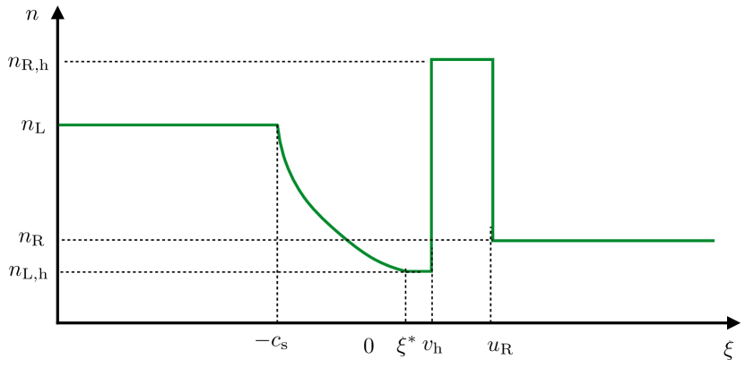
Figure 9: A qualitative sketch of the charge density $n(\xi)$ in the hydrodynamic Riemann problem for a charged fluid without momentum relaxtion.

Such a shock must move at $v_{\mathrm{h}}$, the velocity of the fluid in the steady state. This follows directly from studying the charge conservation equation in the local rest frame of the fluid, in the uniform boosted region between the rarefaction and shock waves. This slowly moving shock wave will also exhibit diffusive broadening, analogous to the discussion in Section III. Only at late times will this diffusive correction to the NESS be convected away; hence, numerically detecting this NESS may require some care. In the special case where $P_{\mathrm{L}}=P_{\mathrm{R}}$, the dynamics is entirely governed by (nonlinear) charge diffusion. In this case we do not expect a NESS with a non-zero charge current to appear as $t\rightarrow\infty$; with $P_{L}=P_{R}$ the energy current and the fluid velocity is zero, hence $J^{x}=nu^{x}=0$.

For a discussion of entropy balance for the right-moving shock wave, see Appendix B.

VI Discussion and Conclusions

In this manuscript we have examined the non-equilibrium energy flow between quantum critical heat baths in arbitrary dimensions. We have shown that it is necessary to consider both shock waves and rarefaction waves in order to describe the steady state energy flow in $d>1$. This yields minor corrections to the numerical value of $J_{\mathrm{E}}$ in the resulting NESS, compared to our previous work Bhaseen et al. (2015). However, there is a qualitative change in the approach to the NESS for large temperature ratios $T_{L}/T_{R}>\Gamma$, where $\Gamma\approx 3.459$ in $d=2$ and $\Gamma\approx 2.132$ in $d=3$. We have also discussed extensions of our previous work to account for viscous broadening of shock waves, and the generalization of our hydrodynamic solution to inhomogeneous fluids as well as charged fluids. Although the exact analytical characterization of the NESS presented in Bhaseen et al. (2015) has been modified in $d>1$, other aspects of the hydrodynamic discussion – including the robustness of $J_{\mathrm{E}}$ against perturbations inhomogeneous in the transverse spatial directions Bhaseen et al. (2015) – are unchanged.

Though our focus in this paper has been on the appearance of a non-equilibrium steady-state, we hope to return to the quantum and thermal fluctuations of this energy current, captured by higher point correlation functions of $J_{\mathrm{E}}$. In the idealized two-shock solution we showed that all higher order moments of the (total) energy current in the NESS are recursively related to the average (total) current (across the contact interface). These extended fluctuation relations (EFR) are exact in 1+1 dimensional conformal theories Bernard and Doyon (2012), and are asymptotically correct in free field theories in $d>1$ Bernard and Doyon (2013); Doyon et al. (2015), where the dynamics is qualitatively similar to rarefaction waves. It will be interesting to revisit the arguments for deriving the EFRs in higher dimensional systems, presented in [12], in the light of our new hydrodynamic results for $T_{\rm L}/T_{\rm R}>\Gamma$.

Note added: While this manuscript was in preparation, we were informed about similar results obtained in Spillane and Herzog .

Appendix A Perturbative Comparison of Solutions

In this Appendix we compute the properties of the NESS to third order in perturbation theory as a function of the perturbative parameter

$$\delta\equiv\frac{T_{\mathrm{L}}}{T_{\mathrm{R}}}-1.$$ (41)

One finds for the rarefaction-shock solution that

$$T_{\mathrm{h}} =T_{\mathrm{R}}\left[1+\frac{\delta}{2}-\frac{\delta^{2}}{8}+\frac{23+2d-d^{2}}{384}\delta^{3}\right]+\mathrm{O}\left(\delta^{4}\right),$$ (42a)

$$v_{\mathrm{h}} =\sqrt{d}\left[\frac{\delta}{2}-\frac{\delta^{2}}{4}+\frac{65-18d+d^{2}}{384}\delta^{3}\right]+\mathrm{O}\left(\delta^{4}\right).$$ (42b)

For the two-shock solution, one finds instead

$$T_{\mathrm{h}}^{\text{2-shock}} =T_{\mathrm{R}}\left[1+\frac{\delta}{2}-\frac{\delta^{2}}{8}+\frac{\delta^{3}}{16}\right]+\mathrm{O}\left(\delta^{4}\right),$$ (43a)

$$v_{\mathrm{h}}^{\text{2-shock}} =\sqrt{d}\left[\frac{\delta}{2}-\frac{\delta^{2}}{4}+\frac{33-10d+d^{2}}{192}\delta^{3}\right]+\mathrm{O}\left(\delta^{4}\right).$$ (43b)

Note that deviations between the two solutions occur only at $\mathrm{O}(\delta^{3})$, and for $d>1$. In addition, the change in the coefficients is quite small for the physical dimensions of $d=2,3$.

An alternative way to write these equations is to note that $T_{\mathrm{h}}^{\text{2-shock}}=\sqrt{T_{\mathrm{L}}T_{\mathrm{R}}}$ Bhaseen et al. (2015). Using this in (42a) we may recast the rarefaction-shock solution in the form

$$T_{\mathrm{h}}=\sqrt{T_{\mathrm{L}}T_{\mathrm{R}}}\left(1-\frac{(d-1)^{2}}{384}\delta^{3}+\mathrm{O}(\delta^{4})\right).$$ (44)

It is readily seen that $T_{\mathrm{h}}=\sqrt{T_{\mathrm{L}}T_{\mathrm{R}}}$ in $d=1$, but it receives cubic corrections in $\delta$ for $d\neq 1$. Similarly,

$$v_{\mathrm{h}}=v_{\mathrm{h}}^{\text{2-shock}}\left(1-\frac{(d-1)^{2}}{192}\delta^{2}+\mathrm{O}(\delta^{3})\right).$$ (45)

Again, the results for the rarefaction-shock and two-shock solutions coincide in $d=1$, but quadratic corrections in $\delta$ appear for $d\neq 1$.

Appendix B Entropy Change Across The Right-Moving Shock

In this Appendix, we demonstrate that the entropy change across the right-moving shock remains compatible with the second law of thermodynamics, even in the presence of charge degrees of freedom. Specifically, we show that the entropy density just to the left of the right-moving shock, $s_{\mathrm{R,h}}$, is larger than the entropy density of the right heat bath, $s_{\mathrm{R}}$, in a scale invariant relativistic charged fluid; see Figs 4 and 9. In this pursuit, we first review some thermodynamic preliminaries.

In equilibrium, the entropy density is constrained by scale invariance and dimensional analysis to have the form

$$s=\epsilon^{d/(d+1)}f\left(\frac{n}{\epsilon^{d/(d+1)}}\right),$$ (46)

where $\epsilon$ is the energy density, $n$ is the charge density and $f$ is a function of the dimensionless ratio

$$\mathcal{X}=n\epsilon^{-d/(d+1)}.$$ (47)

Although the function $f$ is specific to the model under consideration, it satisfies some general properties. For example, charge conjugation symmetry about $n=0$ implies that $f(\mathcal{X})=f(-\mathcal{X})$. Further, using the first law of thermodynamics

$$\mathrm{d}s=\frac{1}{T}\mathrm{d}\epsilon-\frac{\mu}{T}\mathrm{d}n,$$ (48)

we see that $(\partial s/\partial n)_{\epsilon}=-\mu/T$. Using charge conjugation symmetry, we find $f^{\prime}(0)=0$, as $\mu=0$ when $n=0$. More generally, we conclude that $f^{\prime}(\mathcal{X})>0$ if $\mathcal{X}<0$ and $f^{\prime}(\mathcal{X})<0$ if $\mathcal{X}>0$, corresponding to $f(\mathcal{X})$ having a maximum at $\mathcal{X}=0$.

Without loss of generality we may take $\mathcal{X}_{\mathrm{R}}>0$, due to charge conjugation symmetry. In order to show that $s_{\mathrm{R,h}}-s_{\mathrm{R}}\geq 0$, it is sufficient to show that $f(\mathcal{X}_{\mathrm{R,h}})\geq f(\mathcal{X}_{\mathrm{R}})$, since $\epsilon_{\mathrm{R,h}}>\epsilon_{\mathrm{R}}$. In Fig. 10 we plot the ratio $\mathcal{X}_{\mathrm{R,h}}/\mathcal{X}_{\mathrm{R}}$ in $d=2,3$, as obtained from Eqs. (17) and (40) using our numerical values for $v_{\mathrm{h}}$ and $u_{\mathrm{R}}$. It is readily seen that $\mathcal{X}_{\mathrm{R,h}}/\mathcal{X}_{\mathrm{R}}\leq 1$. It follows that $f(\mathcal{X}_{\mathrm{R,h}})\geq f(\mathcal{X}_{\mathrm{R,h}})$, and thus $s_{\mathrm{R,h}}-s_{\mathrm{R}}\geq 0$, as required.

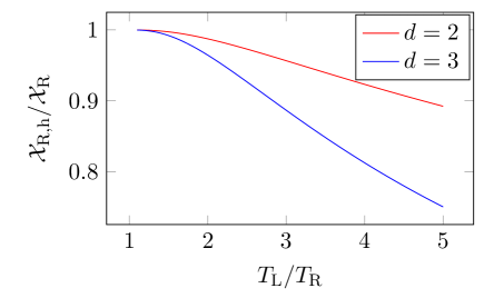
Figure 10: A comparison of the dimensionless ratios $\mathcal{X}_{\mathrm{R,h}}$ and $\mathcal{X}_{\mathrm{R}}$ to the left and the right of the right-moving shock. The ratio $\mathcal{X}_{\mathrm{R,h}}/\mathcal{X}_{\mathrm{R}}$ is always less than unity for $d=2,3$.

References

- Polkovnikov et al. (2011) A. Polkovnikov, K. Sengupta, Alessandro A. Silva, and M. Vengalattore, “Colloquium: Nonequilibrium dynamics of closed interacting quantum systems,” Rev. Mod. Phys., 83, 863 (2011).
- Kinoshita et al. (2006) T. Kinoshita, T. Wenger, and D. S. Weiss, “A quantum Newton’s cradle,” Nature, 440, 900 (2006).
- Rigol et al. (2007) M. Rigol, V. Dunjko, V. Yurovsky, and M. Olshanii, “Relaxation in a Completely Integrable Many-Body Quantum System: An Ab Initio Study of the Dynamics of the Highly Excited States of 1D Lattice Hard-Core Bosons,” Phys. Rev. Lett., 98, 050405 (2007).
- Rigol et al. (2008) M. Rigol, V. Dunjko, and M. Olshanii, “Thermalization and its mechanism for generic isolated quantum systems,” Nature, 452, 854 (2008).
- Rigol (2009) M. Rigol, “Breakdown of thermalization in finite one-dimensional systems,” Phys. Rev. Lett., 103, 100403 (2009).
- Cao et al. (2011) C. Cao, E. Elliott, J. Joseph, H. Wu, J. Petricka, T. Schäfer, and J. E. Thomas, “Universal quantum viscosity in a unitary Fermi gas,” Science, 331, 58 (2011).
- de Jong and Molenkamp (1995) M. J. M. de Jong and L. W. Molenkamp, “Hydrodynamic electron flow in high-mobility wires,” Phys. Rev. B, 51, 11389 (1995).
- (8) D. A. Bandurin et al., “Negative local resistance due to viscous electron backflow in graphene,” arXiv:1509.04165 .
- (9) P. J. W. Moll, P. Kushwaha, N. Nandi, B. Schmidt, and A. P. Mackenzie, “Evidence for hydrodynamic electron flow in ,” arXiv:1509.05691 .
- (10) J. Crossno et al., “Observation of the Dirac fluid and the breakdown of the Wiedemann-Franz law in graphene,” arXiv:1509.04713 .
- (11) A. Lucas, J. Crossno, K. C. Fong, P. Kim, and S. Sachdev, “Transport in inhomogeneous quantum critical fluids and in the Dirac fluid in graphene,” arXiv:1510.01738 .
- Bhaseen et al. (2015) M. J. Bhaseen, B. Doyon, A. Lucas, and K. Schalm, “Energy flow in quantum critical systems far from equilibrium,” Nat. Phys., 11, 509 (2015).
- Bernard and Doyon (2012) D. Bernard and B. Doyon, “Energy flow in non-equilibrium conformal field theory,” J. Phys. A: Math. Theor., 45, 362001 (2012).
- Chang et al. (2014) H-C. Chang, A. Karch, and A. Yarom, “An ansatz for one dimensional steady state configurations,” J. Stat. Mech., P06018 (2014).
- Amado and Yarom (2015) I. Amado and A. Yarom, “Black brane steady states,” JHEP, 10, 105 (2015).
- (16) R. Pourhasan, “Non-equilibrium steady state in the hydro regime,” arXiv:1509.01162 .
- Bernard and Doyon (2013) D. Bernard and B. Doyon, “Time-reversal symmetry and fluctuation relations in non-equilibrium quantum steady states,” J. Phys. A: Math. Theor., 46, 372001 (2013).
- Bernard and Doyon (2015) D. Bernard and B. Doyon, “Non-equilibrium steady-states in conformal field theory,” Ann. Henri Poincaré, 16, 113 (2015).
- Cardy (2010) J. Cardy, “The ubiquitous ’ c ’: from the Stefan- Boltzmann law to quantum information,” J. Stat. Mech., P10004 (2010).
- Pendry (1983) J. B. Pendry, “Quantum limits to the flow of information and entropy,” J. Phys. A: Math. Gen., 16, 2161 (1983).
- Sivan and Imry (1986) U. Sivan and Y. Imry, “Multichannel Landauer formula for thermoelectric transport with application to thermopower near the mobility edge,” Phys. Rev. B, 33, 551 (1986).
- Butcher (1990) P. N. Butcher, “Thermal and electrical transport formalism for electronic microstructures with many terminals,” J. Phys. Condens. Matter, 2, 4869 (1990).
- Fazio et al. (1998) R. Fazio, F. W. J. Hekking, and D. E. Khmelnitskii, “Anomalous thermal transport in quantum wires,” Phys. Rev. Lett., 80, 5611 (1998).
- Jezouin et al. (2013) S. Jezouin, F. D. Parmentier, A. Anthore, U. Gennser, A. Cavanna, Y. Jin, and F. Pierre, “Quantum limit of heat flow across a single electronic channel,” Science, 342, 601 (2013).
- Schwab et al. (2000) K. Schwab, E. A. Henriksen, J. M. Worlock, and M. L. Roukes, “Measurement of the quantum of thermal conductance,” Nature, 404, 974 (2000).
- Rego and Kirczenow (1998) L. G. C. Rego and G. Kirczenow, “Quantized thermal conductance of dielectric quantum wires,” Phys. Rev. Lett., 81, 232 (1998).
- Karrasch et al. (2013) C. Karrasch, R. Ilan, and J. E. Moore, “Nonequilibrium thermal transport and its relation to linear response,” Phys. Rev. B, 88, 195129 (2013a).
- Karrasch et al. (2012) C. Karrasch, J. H. Bardarson, and J. E. Moore, “Finite-Temperature Dynamical Density Matrix Renormalization Group and the Drude Weight of Spin- Chains,” Phys. Rev. Lett., 108, 227206 (2012).
- Karrasch et al. (2013) C. Karrasch, J. H. Bardarson, and J. E. Moore, “Reducing the numerical effort of finite-temperature density matrix renormalization group calculations,” New J. Phys., 15, 083031 (2013b).
- Huang et al. (2013) Y. Huang, C. Karrasch, and J. E. Moore, “Scaling of electrical and thermal conductivities in an almost integrable chain,” Phys. Rev. B, 88, 115126 (2013).
- (31) D. Bernard and B. Doyon, “A hydrodynamic approach to non-equilibrium conformal field theories,” arXiv:1507.07474 .
- (32) R. Vasseur, C. Karrasch, and J. E. Moore, “Expansion potentials for exact far-from-equilibrium spreading of particles and energy,” arXiv:1507.08603 .
- Abanov and Wiegmann (2005) A. G. Abanov and P. B. Wiegmann, “Quantum hydrodynamics, the quantum Benjamin-Ono equation, and the Calogero model,” Phys. Rev. Lett., 95, 076402 (2005).
- Taub (1948) A. H. Taub, “Relativistic Rankine-Hugoniot equations,” Phys. Rev., 74, 328 (1948).
- Thompson (1986) K. W. Thompson, “The special relativistic shock tube,” J. Fluid. Mech., 171, 365 (1986).
- Lax (1957) P. D. Lax, “Hyperbolic systems of conservation laws II,” Comm. Pure Appl. Math., 10, 537 (1957).
- Liu (1975) T. P. Liu, “The Riemann problem for general systems of conservation laws,” J. Diff. Equat., 18, 218 (1975).
- Marti and Müller (2003) J. M. Marti and E. Müller, “Numerical hydrodynamics in special relativity,” Living Rev. Relativity, 6, 7 (2003).
- Mach and Pietka (2010) P. Mach and M. Pietka, “Exact solution of the hydrodynamical Riemann problem with nonzero tangential velocities and the ultrarelativistic equation of state,” Phys. Rev. E, 81, 046313 (2010).
- Collura and Martelloni (2014) M. Collura and G. Martelloni, “Non-equilibrium transport in -dimensional non-interacting Fermi gases,” J. Stat. Mech., P08006 (2014).
- Doyon et al. (2015) B. Doyon, A. Lucas, K. Schalm, and M. J. Bhaseen, “Non-equilibrium steady states in the Klein-Gordon theory,” J. Phys. A: Math. Gen., 48, 095002 (2015).
- Landau and Lifshitz (1987) L. D. Landau and E. M. Lifshitz, Fluid Mechanics (Butterworth Heinemann, 1987).
- Lucas (2015) A. Lucas, “Hydrodynamic transport in strongly coupled disordered quantum field theories,” New J. Phys., 17, 113007 (2015).
- Hartnoll et al. (2007) S. A. Hartnoll, P. K. Kovtun, M. Müller, and S. Sachdev, “Theory of the Nernst effect near quantum phase transitions in condensed matter, and in dyonic black holes,” Phys. Rev. B, 76, 144502 (2007).
- Davison (2013) R. A. Davison, “Momentum relaxation in holographic massive gravity,” Phys. Rev. D, 88, 086003 (2013).
- Blake (2015) M. Blake, “Momentum relaxation from the fluid/gravity correspondence,” JHEP, 09, 010 (2015).
- (47) M. Spillane and C. P. Herzog, “Relativistic hydrodynamics and non-equilibrium steady states,” arXiv:1512.09071 .