3D printing dimensional calibration shape: Clebsch Cubic

Author Andrรฉ. F. van der Merwe Department of Industrial Engineering, Stellenbosch University, South Africa, andrevdm@sun.ac.za Janko Bรถhm Department of Mathematics, University of Kaiserslautern, Germany, boehm@mathematik.uni-kl.de Magdaleen S. Marais Department of Mathematics and Applied Mathematics, University of Pretoria, South Africa, magdaleen.marais@up.ac.za
Abstract

3D printing and other layer manufacturing processes are challenged by dimensional accuracy. Several techniques are used to validate and calibrate dimensional accuracy through the complete building envelope. The validation process involves the growing and measuring of a shape with known parameters. The measured result is compared with the intended digital model. Processes with the risk of deformation after time or post processing may find this technique beneficial. We propose to use objects from algebraic geometry as test shapes. A cubic surface is given as the zero set of a $3$rd degree polynomial with $3$ variables. A class of cubics in real $3$D space contains exactly $27$ real lines. We provide a library for the computer algebra system Singular which, from $6$ given points in the plane, constructs a cubic and the lines on it. A surface shape derived from a cubic offers simplicity to the dimensional comparison process, in that the straight lines and many other features can be analytically determined and easily measured using non-digital equipment. For example, the surface contains so-called Eckardt points, in each of which three of the lines intersect, and also other intersection points of pairs of lines. Distances between these intersection points can easily be measured, since the points are connected by straight lines. At all intersection points of lines, angles can be verified. Hence, many features distributed over the build volume are known analytically, and can be used for the validation process. Due to the thin shape geometry the material required to produce an algebraic surface is minimal. This paper is the first in a series that proposes the process chain to first define a cubic with a configuration of lines in a given print volume and then to develop the point cloud for the final manufacturing. Simple measuring techniques are recommended.

1 Introduction

This paper is the first in a series to investigate whether cubic surface shapes, and specifically the Clebsch cubic, can be used in 3D printing build volume accuracy. In this initial paper the phases of development are proposed and the authors attempt to determine the mathematical base for calculating with cubic surfaces. Various build volumes, growing techniques and materials may require slight adjustments due to its unique characteristics. However, the basic shape and mathematical approach remains the same for all variants. The ultimate aim is to have a standard Clebsch cubic shape which can be grown on any platform in any material, and in any build volume size. The research phases proposed are an initial analytical mathematical model, then an engine which converts from the analytical model to a point cloud, then a digital domain simulated growth, followed by an actual hardware printing phase, and lastly a reverse engineering phase. The initial mathematical model is developed from ground rules to provide others the fundamental information for parallel development. The input to the mathematical model, based on the mathematical formulations found by Clebsch and others, is the extent of the build volume. The open source computer algebra system Singular is used for this conversion. The outputs from the mathematical model is a three dimensional shape in analytical mathematical formulation, the formulas for 27 straight lines, the coordinates of the points where the lines cross, and the angles between the lines. After printing, the line straightness is one indicator of the dimensional accuracy. Another indicator is the angles between lines. The coordinate positioning of the cross points, and the thickness of the cubicโ€™s vanes could also be measures. This model is developed and suggested in the second part of this paper. The engine which converts the analytical mathematical formulation to a printable point cloud would typically be programmed in Matlab and later in C++. The inputs are the three dimensional mathematical shape of the Clebsch cubic, and the formulas of the 27 straight lines that we want to use as part of the dimensional accuracy measurement. Note that the straight lines will have to be highlighted in some way for the reverse engineering process to pick it up. Several ways could be used to highlight the lines: generating cylinders around the lines with diameter larger than the cubics vane thickness, thinning the vanes along the lines, or perforating the vanes along the lines, are examples. The output of this engine would be a point cloud in an STL format or similar. In phase three of this project we would attempt to compare the point cloud with the initial analytical line formulas. This comparison can be done on a CAD platform, but would typically be a manual process. Several alternatives of the previous phases will be evaluated for accuracy. All work up to this point is in the digital domain. This phase is to ensure accuracy and robustness of self developed tools by comparison with trusted commercially available CAD platforms. The output of this phase is a report which defines constraints and extents within which these techniques are deemed accurate in the digital domain. Phase four will see the growing of hard copies in various materials on various platforms. This phase will report on any manufacturing issues on any of the platforms using the extent of materials chosen. Phase five will reverse engineer hardware shapes to compare with the initial intended analytical shape. In this phase it will be determined to what extent the use of the $27$ straight lines and their angles is an indication of dimensional accuracy of the process. This phase will seek to propose an economical method of measuring dimensional accuracy of the complete building envelope. This paper starts with the mathematical setup on which the description of the cubic and the lines are based. Then a reference to the mathematical origins of the cubic surfaces is made, followed by the derivation of the surface equation and the lines. Finally an example output from the computer algebra library and explicit data for the Clebsch cubic is given.

2 Algebraic varieties

We first set the mathematical framework used to describe the cubic and the lines on it. Let $K$ be either the real numbers $\mathbb{R}$ or the complex numbers $\mathbb{C}$. The set of lines through the origin in $K^{n+1}$ is called projective space and is denoted $\mathbb{P}_{K}^{n}$. We will write $(x_{0}:\ldots:x_{n})$ for the line with direction (x0,โ€ฆ,xn)โ‰ 0subscript๐‘ฅ0โ€ฆsubscript๐‘ฅ๐‘›0(x_{0},\ldots,x_{n})\neq 0. There is an inclusion of usual $n$-space to projective space

KnโŸถโ„™Kn,ย (x1,โ€ฆ,xn)โŸผ(1:x1:โ€ฆ:xn).K^{n}\longrightarrow\mathbb{P}_{K}^{n}\text{, }\hskip 8.53581pt(x_{1},\ldots,x_{n})\longmapsto(1:x_{1}:\ldots:x_{n}).

This map is referred to as an affine chart. The complement of the image is called the plane at infinity (the horizon in a perspective drawing). An algebraic variety $V(f_{1},\ldots,f_{r})\subset\mathbb{P}_{K}^{n}$ is the common zero set of homogeneous polynomials $f_{i}\in K[x_{0},\ldots,x_{n}]$.

Algebraic varieties are studied in algebraic geometry, which forms a central branch of classical mathematics. It has important applications, e.g., in cryptography, robotics, and computational biology. Algebraic varieties have the advantage over zero sets of non-polynomial equations that they can easily be handled by the means of computer algebra. For computing with polynomials we make use of the open-source computer algebra system Singular [8]. Using projective space in the development of the theory, avoids the problem that some features of an algebraic variety (e.g. a line on it) may be contained in the plane at infinity. For an introduction to algebraic geometry, computer algebra, and its applications see, e.g. [6].

3 Historic overview and derivation of the fundamental properties of cubic hypersurfaces

Starting in the second half of the $19$th century, Clebsch,ย Klein, Salmon, Coble and many other mathematicians investigated cubic surfaces in $\mathbb{P}_{\mathbb{C}}^{3}$, which are given by a single $3$rd degree polynomial. In $1849$, Arthur Cayley [2] and George Salmon [11] found:

Theorem 3.1.

Every smooth cubic surface in $\mathbb{P}_{\mathbb{C}}^{3}$ contains exactly $27$ lines.

Here smooth means, that $C$ has in every point a well-defined tangent plane. In algebraic geometry there is a process, called blowup, which replaces in a variety a given point by a line and is a $1:1$ map everywhere else. In $1871$ Alfred Clebsch [4] proved (see also [3]):

Theorem 3.2.

Every smooth cubic surface in $\mathbb{P}_{\mathbb{C}}^{3}$ is the blowup of $\mathbb{P}_{\mathbb{C}}^{2}$ in $6$ points.

In the following, let $P_{1},\ldots,P_{6}\in\mathbb{P}_{K}^{2}$ be points in general position, that is, no three are on a line and not all of them on a conic.

Remark 3.3.

The homogeneous linear polynomial

$$l_{i,j}(t):=\det\left(P_{i},P_{j},t\right):=\det\left(\begin{array}[c]{rrr}P_{i,0}&P_{j,0}&t_{0}\\ P_{i,1}&P_{j,1}&t_{1}\\ P_{i,2}&P_{j,2}&t_{2}\end{array}\right)\in K[t_{0},t_{1},t_{2}]$$

defines in $\mathbb{P}_{K}^{2}$ the line through $P_{i}$ and $P_{j}$.

Proposition 3.4.

[5] The blowup $C=C_{(P_{1},\ldots,P_{6})}$ of $\mathbb{P}_{K}^{2}$ in the points $P_{i}$ is the smallest algebraic variety (with respect to inclusion) containing the image of

$\varphi_{(P_{1},\ldots,P_{6})}:$ $\mathbb{P}_{K}^{2}\backslash\{P_{1},\ldots P_{6}\}$ $\longrightarrow$ $\mathbb{P}_{K}^{5}$
$(t_{0}:t_{1}:t_{2})$ $\longmapsto$ $\left(\varphi_{0}(t):\ldots:\varphi_{5}(t)\right)$
ย ย ย ย 

(defined on $\mathbb{P}_{K}^{2}$ except at the points $P_{1},\ldots P_{6}$), where

$\varphi_{0}=l_{2,5}l_{1,3}l_{4,6}+l_{5,1}l_{4,2}l_{3,6}+l_{1,4}l_{3,5}l_{2,6}+l_{4,3}l_{2,1}l_{5,6}+l_{3,2}l_{5,4}l_{1,6}$
$\varphi_{1}=l_{5,3}l_{1,2}l_{4,6}+l_{1,4}l_{2,3}l_{5,6}+l_{2,5}l_{3,4}l_{1,6}+l_{3,1}l_{4,5}l_{2,6}+l_{4,2}l_{5,1}l_{3,6}$
$\varphi_{2}=l_{5,3}l_{4,1}l_{2,6}+l_{3,4}l_{2,5}l_{1,6}+l_{4,2}l_{1,3}l_{5,6}+l_{2,1}l_{5,4}l_{3,6}+l_{1,5}l_{3,2}l_{4,6}$
$\varphi_{3}=l_{4,5}l_{3,1}l_{2,6}+l_{5,3}l_{2,4}l_{1,6}+l_{4,1}l_{2,5}l_{3,6}+l_{3,2}l_{1,5}l_{4,6}+l_{2,1}l_{4,3}l_{5,6}$
$\varphi_{4}=l_{3,1}l_{2,4}l_{5,6}+l_{1,2}l_{5,3}l_{4,6}+l_{2,5}l_{4,1}l_{3,6}+l_{5,4}l_{3,2}l_{1,6}+l_{4,3}l_{1,5}l_{2,6}$
$\varphi_{5}=l_{4,2}l_{3,5}l_{1,6}+l_{2,3}l_{1,4}l_{5,6}+l_{3,1}l_{5,2}l_{4,6}+l_{1,5}l_{4,3}l_{2,6}+l_{5,4}l_{2,1}l_{3,6}$.
ย ย ย ย 
Remark 3.5.

The Clebsch cubic, given in [4, Ch. 16], is obtained by applying this construction to the points in general position

$P_{1}=(0:1:-g)$ $P_{3}=(1:g:0)$ $P_{5}=(0:1:g)$
$P_{2}=(g:0:1)$ $P_{4}=(1:-g:0)$ $P_{6}=(-g:0:1)$,

where $g=\frac{1+\sqrt{5}}{2}$ is the golden ratio. These points correspond to the diagonals in an icosahedron. The Clebsch cubic with $K=\mathbb{R}$ contains $27$ real lines.

Remark 3.6.

The number

$$\left|i,j;k,l;m,n\right|=\det\left(\begin{array}[c]{rr}\det\left(P_{i},P_{j},P_{m}\right)&\det\left(P_{i},P_{j},P_{n}\right)\\ \det\left(P_{k},P_{l},P_{m}\right)&\det\left(P_{k},P_{l},P_{n}\right)\end{array}\right)\text{,}$$

vanishes if the lines defined by $l_{i,j}(t)$, $l_{k,l}(t)$ and $l_{m,n}(t)$ in $\mathbb{P}_{K}^{2}$ meet in one point.

Theorem 3.7.

[5, 7] Consider the skew-symmetric matrix

$$(A_{i,j})=\left({\footnotesize\begin{array}[c]{cccccc}0&\left|1,5;2,4;3,6\right|&\left|1,4;3,5;2,6\right|&\left|1,2;4,3;5,6\right|&\left|2,3;4,5;1,6\right|&\left|1,3;5,2;4,6\right|\\ &0&\left|2,5;3,4;1,6\right|&\left|1,3;5,4;2,6\right|&\left|1,2;3,5;4,6\right|&\left|1,4;2,3;5,6\right|\\ &&0&\left|1,5;3,2;4,6\right|&\left|1,3;2,4;5,6\right|&\left|1,2;4,5;3,6\right|\\ &&&0&\left|1,4;5,2;3,6\right|&\left|2,4;3,5;1,6\right|\\ &\overline{\phantom{xx}}&&&0&\left|1,5;3,4;2,6\right|\\ &&&&&0\end{array}}\right)\in K^{6\times 6}$$

where the entries are defined as in Remark 3.6, and write for the sum of the entries of the $i$-th row

$$a_{i}=\sum_{j=1}^{6}A_{i,j}\text{.}$$

Then $C$ is given by the equations

$\displaystyle x_{0}^{3}+\ldots+x_{5}^{3}$ $\displaystyle=0$
$\displaystyle x_{0}+\ldots+x_{5}$ $\displaystyle=0$
$\displaystyle a_{0}\cdot x_{0}+\ldots+a_{5}\cdot x_{5}$ $\displaystyle=0\text{.}$
Remark 3.8.

Using the ordering of the $P_{i}$ from Remark 3.5, we obtain for the Clebsch cubic surface $a_{0}=a_{1}=a_{2}=a_{3}=a_{4}=1$ and $a_{5}=-5$.

Remark 3.9.

For a subset $S\subset\mathbb{P}_{\mathbb{C}}^{n}$ we define $I(S)$ as the ideal of all $f\in\mathbb{C}[x_{0},\ldots,x_{n}]$ with $f(x)=0$ for all $x\in S$. So $V(I(S))$ is the smallest algebraic variety (with respect to inclusion) containing $S$. The ideal generated by the $\varphi_{i}$ is

$$\left\langle\varphi_{0},\ldots,\varphi_{5}\right\rangle=I(P_{1})\cap...\cap I(P_{6})\text{.}$$

With the ring homomorphism

$\psi_{(P_{1},\ldots,P_{6})}:$ $\mathbb{C}[x_{0},\ldots,x_{5}]$ $\longrightarrow$ $\mathbb{C}[t_{0},t_{1},t_{2}]$
$x_{i}$ $\longmapsto$ $\varphi_{i}$
ย ย ย ย ย ย 

we have

$$I(C)=\ker\psi_{(P_{1},\ldots,P_{6})}=\left\langle x_{0}^{3}+...+x_{5}^{3},\text{ }x_{0}+...+x_{5},\text{ }a_{0}x_{0}+...+a_{5}x_{5}\right\rangle\text{.}$$
Remark 3.10.

Eliminating two variables by the two linear equations, $C$ can be considered as a subset of $\mathbb{P}_{K}^{3}$.

Note that a plane intersects $C$ in an irreducible plane cubic, a union of a conic and a line, or in three lines.

Definition 3.11.

A tritangent plane $H$ to $C$ is a plane, such that $H\cap C$ consists out of three lines.

Remark 3.12.

A tritangent plane $H$ to $C$ is called generic if the three lines pairwise intersect in three distinct points. Then $H$ is tangent to $C$ in each of the three points.

If $H$ is not generic, then the three lines on $C$ intersect in a single point. This point is called an Eckardt point of $C$.

Since in an Eckardt point the three lines are tangent to $C$, they are coplanar, hence, lie on a tritangent plane. So, the Eckardt points are in one-to-one correspondence to the non-generic tritangent planes.

Theorem 3.13.

[5, 2] There are $45$ tritangent planes to $C$:

  1. 1.

    Of these, $15$ are given by the equations

    $$x_{i}+x_{j}=0$$

    for $0\leq i<j\leq 5$.

  2. 2.

    Write $M$ for the set of $2$-element subsets of $\{1,\ldots,6\}$, and $S(M)$ for the set of permutations of $M$. The remaining $30$ tritangent planes are then

    $$\left(m_{i,j}-d_{2}\right)\cdot(x_{i}+x_{j})-(m_{k,l}+d_{2})\cdot(x_{k}+x_{l})=0$$

    where

    {i,j}{k,l}{m,n}โˆˆSโ€‹(M){i,j}{k,l}{m,n}๐‘†๐‘€\leavevmode\hbox to87.32pt{\vbox to58.24pt{\pgfpicture\makeatletter\hbox{\hskip 42.20247pt\lower-32.83188pt\hbox to0.0pt{\pgfsys@beginscope\pgfsys@invoke{ }\definecolor{pgfstrokecolor}{rgb}{0,0,0}\pgfsys@color@rgb@stroke{0}{0}{0}\pgfsys@invoke{ }\pgfsys@color@rgb@fill{0}{0}{0}\pgfsys@invoke{ }\pgfsys@setlinewidth{0.4pt}\pgfsys@invoke{ }\nullfont\hbox to0.0pt{\pgfsys@beginscope\pgfsys@invoke{ } {}{{}}\hbox{\hbox{{\pgfsys@beginscope\pgfsys@invoke{ }{{}{{}}{}{}} \pgfsys@invoke{\lxSVG@closescope }\pgfsys@endscope}}} {}{{}}\hbox{\hbox{{\pgfsys@beginscope\pgfsys@invoke{ }{{}{{}}{}{}} \pgfsys@invoke{\lxSVG@closescope }\pgfsys@endscope}}} {}{{}}\hbox{\hbox{{\pgfsys@beginscope\pgfsys@invoke{ }{{}{{}}{}{}} \pgfsys@invoke{\lxSVG@closescope }\pgfsys@endscope}}} {{}}{{}}\hbox{\hbox{{\pgfsys@beginscope\pgfsys@invoke{ }{{}{}{{ {}{}}}{ {}{}} {{}{{}}}{{}{}}{}{{}{}} { }{{{{}}\pgfsys@beginscope\pgfsys@invoke{ }\pgfsys@transformcm{1.0}{0.0}{0.0}{1.0}{-9.30559pt}{14.57182pt}\pgfsys@invoke{ }\hbox{{\definecolor{pgfstrokecolor}{rgb}{0,0,0}\pgfsys@color@rgb@stroke{0}{0}{0}\pgfsys@invoke{ }\pgfsys@color@rgb@fill{0}{0}{0}\pgfsys@invoke{ }\hbox{{\{i,j\}}} }}\pgfsys@invoke{\lxSVG@closescope }\pgfsys@endscope}}} \pgfsys@invoke{\lxSVG@closescope }\pgfsys@endscope}}} {{}}{{}}\hbox{\hbox{{\pgfsys@beginscope\pgfsys@invoke{ }{{}{}{{ {}{}}}{ {}{}} {{}{{}}}{{}{}}{}{{}{}} { }{{{{}}\pgfsys@beginscope\pgfsys@invoke{ }\pgfsys@transformcm{1.0}{0.0}{0.0}{1.0}{-38.86946pt}{-19.57182pt}\pgfsys@invoke{ }\hbox{{\definecolor{pgfstrokecolor}{rgb}{0,0,0}\pgfsys@color@rgb@stroke{0}{0}{0}\pgfsys@invoke{ }\pgfsys@color@rgb@fill{0}{0}{0}\pgfsys@invoke{ }\hbox{{\{k,l\}}} }}\pgfsys@invoke{\lxSVG@closescope }\pgfsys@endscope}}} \pgfsys@invoke{\lxSVG@closescope }\pgfsys@endscope}}} {{}}{{}}\hbox{\hbox{{\pgfsys@beginscope\pgfsys@invoke{ }{{}{}{{ {}{}}}{ {}{}} {{}{{}}}{{}{}}{}{{}{}} { }{{{{}}\pgfsys@beginscope\pgfsys@invoke{ }\pgfsys@transformcm{1.0}{0.0}{0.0}{1.0}{15.11938pt}{-19.57182pt}\pgfsys@invoke{ }\hbox{{\definecolor{pgfstrokecolor}{rgb}{0,0,0}\pgfsys@color@rgb@stroke{0}{0}{0}\pgfsys@invoke{ }\pgfsys@color@rgb@fill{0}{0}{0}\pgfsys@invoke{ }\hbox{{\{m,n\}}} }}\pgfsys@invoke{\lxSVG@closescope }\pgfsys@endscope}}} \pgfsys@invoke{\lxSVG@closescope }\pgfsys@endscope}}} { {}{}{}}{}{ {}{}{}}{}{ {}{}{}}{}\hbox{\hbox{\hbox{\hbox{{\pgfsys@beginscope\pgfsys@invoke{ } { {}{}{}}{}{ {}{}{}}{ {}{}{}}{{{{}}{{}}{{}}{{}}}{{{{}}{ {}{}}{}{}{{}{}}}} }{{{{}}{{}}{{}}{{}}{{}}}{{{{}}{ {}{}}{}{}{{}{}}}} }{{}{}}{{}} {}{}{}{{{}}{{}}{{}}} {{{}}{{}}{{}}} {}{{}}{}{{}}{}{{}}{}{}{}{}{}{}{}{{}}{}{{ {\pgfsys@beginscope\pgfsys@setdash{}{0.0pt}\pgfsys@roundjoin{} {}{}{} {}{}{} {}{}{} \pgfsys@moveto{0.79999pt}{0.0pt}\pgfsys@curveto{-0.2pt}{0.2pt}{-1.19998pt}{0.59999pt}{-2.39996pt}{1.29997pt}\pgfsys@curveto{-1.19998pt}{0.4pt}{-1.19998pt}{-0.4pt}{-2.39996pt}{-1.29997pt}\pgfsys@curveto{-1.19998pt}{-0.59999pt}{-0.2pt}{-0.2pt}{0.79999pt}{0.0pt}\pgfsys@closepath\pgfsys@fillstroke\pgfsys@endscope}} }{}{}{{}}{{ {\pgfsys@beginscope\pgfsys@setdash{}{0.0pt}\pgfsys@rectcap{} {} \pgfsys@moveto{0.09999pt}{-2.59999pt}\pgfsys@lineto{0.09999pt}{2.59999pt}\pgfsys@stroke\pgfsys@endscope}} }{}{}{{}}\pgfsys@moveto{-13.10843pt}{12.21896pt}\pgfsys@curveto{-21.72139pt}{8.03574pt}{-26.27332pt}{1.31105pt}{-26.83566pt}{-6.54393pt}\pgfsys@stroke\pgfsys@invoke{ }{{}{{}}{}{}{{}}{{{}}{{{}}{\pgfsys@beginscope\pgfsys@invoke{ }\pgfsys@transformcm{0.89952}{0.43689}{-0.43689}{0.89952}{-13.10844pt}{12.21895pt}\pgfsys@invoke{ }\pgfsys@invoke{ \lxSVG@closescope }\pgfsys@invoke{\lxSVG@closescope }\pgfsys@endscope}}{{}}}}{{}{{}}{}{}{{}}{{{}}{{{}}{\pgfsys@beginscope\pgfsys@invoke{ }\pgfsys@transformcm{-0.07141}{-0.99745}{0.99745}{-0.07141}{-26.83565pt}{-6.54393pt}\pgfsys@invoke{ }\pgfsys@invoke{ \lxSVG@closescope }\pgfsys@invoke{\lxSVG@closescope }\pgfsys@endscope}}{{}}}}\hbox{\hbox{{\pgfsys@beginscope\pgfsys@invoke{ }{{}{}{{{}{}}}{{}{}} {{}{{}}}{{}{}}{}{{}{}} { }{{{{}}\pgfsys@beginscope\pgfsys@invoke{ }\pgfsys@transformcm{1.0}{0.0}{0.0}{1.0}{-26.50813pt}{3.98141pt}\pgfsys@invoke{ }\hbox{{\definecolor{pgfstrokecolor}{rgb}{0,0,0}\pgfsys@color@rgb@stroke{0}{0}{0}\pgfsys@invoke{ }\pgfsys@color@rgb@fill{0}{0}{0}\pgfsys@invoke{ }\hbox{} }}\pgfsys@invoke{\lxSVG@closescope }\pgfsys@endscope}}} \pgfsys@invoke{\lxSVG@closescope }\pgfsys@endscope}}} \pgfsys@invoke{\lxSVG@closescope }\pgfsys@endscope}}}\hbox{{\pgfsys@beginscope\pgfsys@invoke{ } { {}{}{}}{}{ {}{}{}}{ {}{}{}}{{{{}}{{}}{{}}{{}}}{{{{}}{ {}{}}{}{}{{}{}}}} }{{{{}}{{}}{{}}{{}}{{}}}{{{{}}{ {}{}}{}{}{{}{}}}} }{{}{}}{{}} {}{}{}{{{}}{{}}{{}}} {{{}}{{}}{{}}} {}{{}}{}{{}}{}{{}}{}{}{}{}{}{}{}{{}}{}{}{}{}{{}}{}{}{}{{}}\pgfsys@moveto{-14.24588pt}{-25.27495pt}\pgfsys@curveto{-5.0456pt}{-30.79962pt}{4.02837pt}{-30.95564pt}{11.92636pt}{-26.5749pt}\pgfsys@stroke\pgfsys@invoke{ }{{}{{}}{}{}{{}}{{{}}{{{}}{\pgfsys@beginscope\pgfsys@invoke{ }\pgfsys@transformcm{-0.85732}{0.5148}{-0.5148}{-0.85732}{-14.24586pt}{-25.27496pt}\pgfsys@invoke{ }\pgfsys@invoke{ \lxSVG@closescope }\pgfsys@invoke{\lxSVG@closescope }\pgfsys@endscope}}{{}}}}{{}{{}}{}{}{{}}{{{}}{{{}}{\pgfsys@beginscope\pgfsys@invoke{ }\pgfsys@transformcm{0.8745}{0.48505}{-0.48505}{0.8745}{11.92636pt}{-26.57492pt}\pgfsys@invoke{ }\pgfsys@invoke{ \lxSVG@closescope }\pgfsys@invoke{\lxSVG@closescope }\pgfsys@endscope}}{{}}}}\hbox{\hbox{{\pgfsys@beginscope\pgfsys@invoke{ }{{}{}{{{}{}}}{{}{}} {{}{{}}}{{}{}}{}{{}{}} { }{{{{}}\pgfsys@beginscope\pgfsys@invoke{ }\pgfsys@transformcm{1.0}{0.0}{0.0}{1.0}{-4.01793pt}{-29.49887pt}\pgfsys@invoke{ }\hbox{{\definecolor{pgfstrokecolor}{rgb}{0,0,0}\pgfsys@color@rgb@stroke{0}{0}{0}\pgfsys@invoke{ }\pgfsys@color@rgb@fill{0}{0}{0}\pgfsys@invoke{ }\hbox{} }}\pgfsys@invoke{\lxSVG@closescope }\pgfsys@endscope}}} \pgfsys@invoke{\lxSVG@closescope }\pgfsys@endscope}}} \pgfsys@invoke{\lxSVG@closescope }\pgfsys@endscope}}}\hbox{{\pgfsys@beginscope\pgfsys@invoke{ } { {}{}{}}{}{ {}{}{}}{ {}{}{}}{{{{}}{{}}{{}}{{}}}{{{{}}{ {}{}}{}{}{{}{}}}} }{{{{}}{{}}{{}}{{}}{{}}}{{{{}}{ {}{}}{}{}{{}{}}}} }{{}{}}{{}} {}{}{}{{{}}{{}}{{}}} {{{}}{{}}{{}}} {}{{}}{}{{}}{}{{}}{}{}{}{}{}{}{}{{}}{}{}{}{}{{}}{}{}{}{{}}\pgfsys@moveto{26.95706pt}{-8.23961pt}\pgfsys@curveto{26.27332pt}{1.31105pt}{21.72139pt}{8.03574pt}{14.63762pt}{11.47626pt}\pgfsys@stroke\pgfsys@invoke{ }{{}{{}}{}{}{{}}{{{}}{{{}}{\pgfsys@beginscope\pgfsys@invoke{ }\pgfsys@transformcm{0.07141}{-0.99745}{0.99745}{0.07141}{26.95705pt}{-8.2396pt}\pgfsys@invoke{ }\pgfsys@invoke{ \lxSVG@closescope }\pgfsys@invoke{\lxSVG@closescope }\pgfsys@endscope}}{{}}}}{{}{{}}{}{}{{}}{{{}}{{{}}{\pgfsys@beginscope\pgfsys@invoke{ }\pgfsys@transformcm{-0.89952}{0.43689}{-0.43689}{-0.89952}{14.63762pt}{11.47626pt}\pgfsys@invoke{ }\pgfsys@invoke{ \lxSVG@closescope }\pgfsys@invoke{\lxSVG@closescope }\pgfsys@endscope}}{{}}}}\hbox{\hbox{{\pgfsys@beginscope\pgfsys@invoke{ }{{}{}{{ {}{}}}{ {}{}} {{}{{}}}{{}{}}{}{{}{}} { }{{{{}}\pgfsys@beginscope\pgfsys@invoke{ }\pgfsys@transformcm{1.0}{0.0}{0.0}{1.0}{26.50813pt}{3.98141pt}\pgfsys@invoke{ }\hbox{{\definecolor{pgfstrokecolor}{rgb}{0,0,0}\pgfsys@color@rgb@stroke{0}{0}{0}\pgfsys@invoke{ }\pgfsys@color@rgb@fill{0}{0}{0}\pgfsys@invoke{ }\hbox{} }}\pgfsys@invoke{\lxSVG@closescope }\pgfsys@endscope}}} \pgfsys@invoke{\lxSVG@closescope }\pgfsys@endscope}}} \pgfsys@invoke{\lxSVG@closescope }\pgfsys@endscope}}} \pgfsys@invoke{\lxSVG@closescope }\pgfsys@endscope{{ {}{}{}{}{}}{{{}}{{}}}}{}{}\hss}\pgfsys@discardpath\pgfsys@invoke{\lxSVG@closescope }\pgfsys@endscope\hss}}\lxSVG@closescope\endpgfpicture}}\in S(M)

    is a $3$-cycle of pairwise disjoint elements of $M$,

    $$d_{2}={\scriptsize\det\left(\begin{array}[c]{rr}\det\left(P_{3},P_{4},P_{1}\right)\cdot\det\left(P_{5},P_{6},P_{1}\right)&\det\left(P_{5},P_{3},P_{1}\right)\cdot\det\left(P_{4},P_{6},P_{1}\right)\\ \det\left(P_{3},P_{4},P_{2}\right)\cdot\det\left(P_{5},P_{6},P_{2}\right)&\det\left(P_{5},P_{3},P_{2}\right)\cdot\det\left(P_{4},P_{6},P_{2}\right)\end{array}\right)}$$

    and

    mi,j=โˆ‘s<tasโ€‹at+2โ€‹(ai2+aj2+aiโ€‹aj)โ€‹,subscript๐‘š๐‘–๐‘—subscript๐‘ ๐‘กsubscript๐‘Ž๐‘ subscript๐‘Ž๐‘ก2superscriptsubscript๐‘Ž๐‘–2superscriptsubscript๐‘Ž๐‘—2subscript๐‘Ž๐‘–subscript๐‘Ž๐‘—,m_{i,j}=\sum_{s<t}a_{s}a_{t}+2(a_{i}^{2}+a_{j}^{2}+a_{i}a_{j})\text{,}

    where $a_{i}$ is as defined in Theorem 3.7.

Remark 3.14.

Possible numbers for Eckardt points are $1,2,3,4,6,9,10,18$. The Clebsch cubic is the unique cubic with $10$ Eckardt points. The Fermat cubic $V(x_{0}^{3}+\ldots+x_{3}^{3})$ is the unique cubic with the maximum possible number of $18$ Eckardt points, however, only $3$ of the lines on the Fermat cubic are defined over $\mathbb{R}$.

Remark 3.15.

Every line on $C$ lies on $5$ tritangent planes. Hence, any line on $C$ is the intersection of the planes $x_{0}+\ldots+x_{5}=0$, $a_{0}x_{0}+...+a_{5}x_{5}=0$ and two tritangent planes (see Remark 3.10).

Remark 3.16.

After permuting the coordinates we may assume that a5โ‰ 0subscript๐‘Ž50a_{5}\neq 0. Then by eliminating $x_{4}$ and $x_{5}$ via the two linear equations of $C$, we obtain $C^{\prime}=V(F)\subset\mathbb{P}_{K}^{3}$ with a homogeneous cubic polynomial $F\in K[x_{0},x_{1},x_{2},x_{3}]$.

Example 3.17.

The Clebsch Cubic is then given by

$$F=x_{0}^{3}+x_{1}^{3}+x_{2}^{3}+x_{3}^{3}-\left(x_{0}+x_{1}+x_{2}+x_{3}\right)^{3}\text{.}$$
Remark 3.18.

For the Clebsch cubic, as well as cubics โ€œcloseโ€ to it in the sense of the position of $P_{1},\ldots,P_{6}$, the transformation

$x_{0}=y_{0}-y_{3}-\sqrt{2}y_{1}$ $x_{2}=y_{0}+y_{3}+\sqrt{2}y_{2}$
$x_{1}=y_{0}-y_{3}+\sqrt{2}y_{1}$ $x_{3}=-y_{0}-y_{3}+\sqrt{2}y_{2}$

of the coordinate system with inverse

$y_{0}=x_{0}+x_{1}+x_{2}-x_{3}$ $y_{2}=\sqrt{2}(x_{2}+x_{3})$
$y_{1}=\sqrt{2}(-x_{0}+x_{1})$ $y_{3}=-x_{0}-x_{1}+x_{2}-x_{3}$
ย ย 

achieves that all $27$ lines, for $K=\mathbb{R}$, are visible in the affine chart

K3โŸถโ„™K3,ย (y1,y2,y3)โŸผ(1:y1:y2:y3).K^{3}\longrightarrow\mathbb{P}_{K}^{3}\text{, }\hskip 8.53581pt(y_{1},y_{2},y_{3})\longmapsto(1:y_{1}:y_{2}:y_{3})\text{.}

Moreover, they all pass through a ball with radius $6$ around 00. In the affine chart we obtain a so-called affine cubic hypersurface $C^{\prime\prime}\subset K^{3}$ given by a single, non-homogeneous $3$rd degree polynomial $f\in K[y_{1},y_{2},y_{3}]$.

4 Implementation in Singular

We have implemented the constructions above in the library cubic.lib [1] for the open-source computer algebra system Singular [8]. For an introduction to the language of Singular see [10]. Specifically, from $6$ points in general position (with coordinates in $\mathbb{Q}$ or an algebraic extension thereof), we give a function to obtain the cubic $C\subset\mathbb{P}_{K}^{5}$, its projection $C^{\prime}\subset\mathbb{P}_{K}^{3}$ and the affine cubic hypersurface $C^{\prime\prime}\subset K^{3}$. Moreover, we compute the parametrizations

$$\mathbb{P}_{K}^{2}\backslash\{P_{1},\ldots,P_{6}\}\longrightarrow C\longrightarrow C^{\prime}$$

and an affine parametrization

$$\mathbb{P}_{K}^{2}\backslash V(\varphi_{0}+\varphi_{1}+\varphi_{2}-\varphi_{3})\longrightarrow C^{\prime\prime}\text{.}$$

Finally, we compute the lines on $C,C^{\prime}$ and $C^{\prime\prime}$ in implicit and parametric form, as well as the Eckardt points. We demonstrate key parts of our library, considering the Clebsch cubic as an example:

Example 4.1.

Our library can be loaded in Singular by:

$>$ LIB "cubic.lib";

We first create a polynomial ring in $4$ variables over the field $\mathbb{Q}[\sqrt{5}]$:

$>$ ring R = (0,a),(x0,x1,x2,x3),dp;

$>$ minpoly = a^2-5;

We specify a list $P$ with the points $P_{1},\ldots,P_{6}$:

$>$ number g = (1 + a)/2;

$>$ list P = vector(0,1,-g), vector(g,0,1), vector(1,g,0), vector(1,-g,0),

vector(0,1,g), vector(-g,0,1);

We compute the equation of $C^{\prime}$:

$>$ poly f =ย cubic(P);

$>$ f;

-3*x0^2*x1-3*x0*x1^2-3*x0^2*x2-6*x0*x1*x2-3*x1^2*x2-3*x0*x2^2-3*x1*x2^2

-3*x0^2*x3-6*x0*x1*x3-3*x1^2*x3-6*x0*x2*x3-6*x1*x2*x3-3*x2^2*x3-3*x0*x3^2

-3*x1*x3^2-3*x2*x3^2

The following command returns a list of all lines on $C^{\prime}$, each specified by $2$ linear equations:

$>$ list L = lines(P);

$>$ L[1];

_[1] = x0 + x1

_[2] = x2 + x3

We compute a list of Eckardt points, each specified by $3$ linear equations:

$>$ list E = EckardtPoints(P);

$>$ E[1];

_[1] = x0

_[2] = x1

_[3] = x2 + x3

Note that, by the commands affineCubic, affineLines and affineEckardtPoints, one can also obtain the affine cubic $C^{\prime\prime}$ and the corresponding lines and Eckardt points, respectively. Moreover, the functions paramLines and affineParamLines compute parametrizations of the lines on $C^{\prime}$ and $C^{\prime\prime}$, respectively.

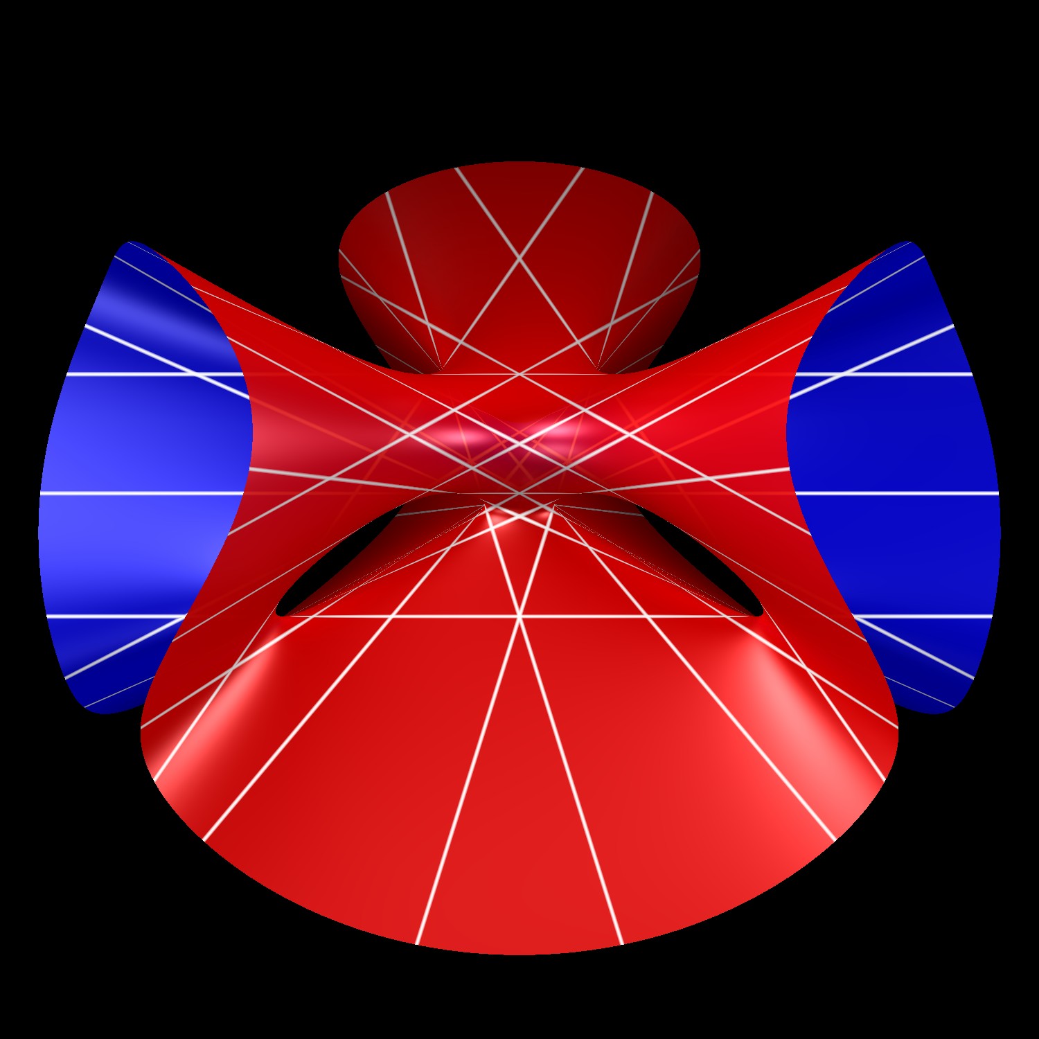
If, in addition to Singular, the program Surf [9] is installed, $C^{\prime\prime}$ can be visualized by:

$>$ LIB "surf.lib";

$>$ plot(affineCubic(P));

It also can plot hyperplane sections of a surface. Hence, we can visualize the lines on the cubic by intersecting with tritangent planes, see Figure 1.

Refer to caption
Figure 1: Lines on the Clebsch cubic

5 Explicit data for the Clebsch cubic

Our program returns the equation for the cubic and derived information for any 6 points in general position in the projective plane (corresponding to lines in 3D space through the origin).

In this section we give the explicit data required for the dimensional comparison process for the Clebsch cubic (i.e. for the choice of the six points given by the diagonals in an icosahedron). In the following let $a=\sqrt{5}$ and $c=\sqrt{2}$. The cubic $C^{\prime\prime}$ is the zero set in $K^{3}$ of the equation

$\displaystyle 2cy_{2}^{3}+2y_{1}^{2}y_{3}-8y_{2}^{2}y_{3}+3cy_{2}y_{3}^{2}-y_{3}^{3}-2y_{1}^{2}+8y_{2}^{2}-10cy_{2}y_{3}+3y_{3}^{2}+3cy_{2}-3y_{3}+1=0\text{.}$

The lines on $C^{\prime\prime}$ given in implicit form (by two linear equations each) as well as their parametrizations (specified as maps Kโ†’K3,sโ†ฆ(ฯˆ1โ€‹(s),ฯˆ2โ€‹(s),ฯˆ3โ€‹(s))formulae-sequenceโ†’๐พsuperscript๐พ3maps-to๐‘ subscript๐œ“1๐‘ subscript๐œ“2๐‘ subscript๐œ“3๐‘ K\rightarrow K^{3},s\mapsto(\psi_{1}(s),\psi_{2}(s),\psi_{3}(s))) are specified in Table 1.

ImplicitParametricโŸจy3โˆ’1,y2โŸฉ(s,0,1)โŸจy3โˆ’1,y2โˆ’2cโŸฉ(s,2c,1)โŸจy3โˆ’1,y2+2cโŸฉ(s,โˆ’2c,1)โŸจy2โˆ’1cโ‹…y3+1c,y1โˆ’1cโ‹…y3โˆ’1cโŸฉ(1cโ‹…s+1c,1cโ‹…sโˆ’1c,s)โŸจy2โˆ’1cโ‹…y3โˆ’1c,y1โˆ’1cโ‹…y3โˆ’3cโŸฉ(1cโ‹…s+3c,1cโ‹…s+1c,s)โŸจy2โˆ’1cโ‹…y3+3c,y1โˆ’1cโ‹…y3+1cโŸฉ(1cโ‹…sโˆ’1c,1cโ‹…sโˆ’3c,s)โŸจy2โˆ’1cโ‹…y3+1c,y1+1cโ‹…y3+1cโŸฉ(โˆ’1cโ‹…sโˆ’1c,1cโ‹…sโˆ’1c,s)โŸจy2โˆ’1cโ‹…y3โˆ’1c,y1+1cโ‹…y3+3cโŸฉ(โˆ’1cโ‹…sโˆ’3c,1cโ‹…s+1c,s)โŸจy2โˆ’1cโ‹…y3+3c,y1+1cโ‹…y3โˆ’1cโŸฉ(โˆ’1cโ‹…s+1c,1cโ‹…sโˆ’3c,s)โŸจy2+1cโ‹…y3+1c,y1+3cโ‹…y3+1cโŸฉ(โˆ’3cโ‹…sโˆ’1c,โˆ’1cโ‹…sโˆ’1c,s)โŸจy2โˆ’3cโ‹…y3+1c,y1โˆ’1cโ‹…y3+1cโŸฉ(1cโ‹…sโˆ’1c,3cโ‹…sโˆ’1c,s)โŸจy2+1cโ‹…y3+1c,y1โˆ’3cโ‹…y3โˆ’1cโŸฉ(3cโ‹…s+1c,โˆ’1cโ‹…sโˆ’1c,s)โŸจy2โˆ’3cโ‹…y3+1c,y1+1cโ‹…y3โˆ’1cโŸฉ(โˆ’1cโ‹…s+1c,3cโ‹…sโˆ’1c,s)โŸจy2,y1โˆ’1cโ‹…y3+1cโŸฉ(1cโ‹…sโˆ’1c,0,s)โŸจy2,y1+1cโ‹…y3โˆ’1cโŸฉ(โˆ’1cโ‹…s+1c,0,s)โŸจy2โˆ’1aโ€‹c+2โ€‹cโ‹…y3+5aโ€‹c,y1+(32โ€‹aโ€‹cโˆ’3โ€‹c)โ‹…y3โˆ’(12โ€‹aโ€‹cโˆ’2โ€‹c)โŸฉ(โˆ’(32โ€‹aโ€‹cโˆ’3โ€‹c)โ‹…s+(12โ€‹aโ€‹cโˆ’2โ€‹c),1aโ€‹c+2โ€‹cโ‹…sโˆ’12โ€‹aโ€‹c,s)โŸจy2โˆ’5aโ€‹cโ‹…y3+1aโ€‹c+2โ€‹c,y1โˆ’11aโ€‹c+4โ€‹cโ‹…y3โˆ’3aโ€‹c+2โ€‹cโŸฉ(11aโ€‹c+4โ€‹cโ‹…s+3aโ€‹c+2โ€‹c,5aโ€‹cโ‹…sโˆ’1aโ€‹c+2โ€‹c,s)โŸจy2+1aโ€‹cโˆ’2โ€‹cโ‹…y3โˆ’5aโ€‹c,y1โˆ’(32โ€‹aโ€‹c+3โ€‹c)โ‹…y3+(12โ€‹aโ€‹c+2โ€‹c)โŸฉ((32โ€‹aโ€‹c+3โ€‹c)โ‹…sโˆ’(12โ€‹aโ€‹c+2โ€‹c),โˆ’1aโ€‹cโˆ’2โ€‹cโ‹…s+12โ€‹aโ€‹c,s)โŸจy2+5aโ€‹cโ‹…y3โˆ’1aโ€‹cโˆ’2โ€‹c,y1+11aโ€‹cโˆ’4โ€‹cโ‹…y3+3aโ€‹cโˆ’2โ€‹cโŸฉ(โˆ’11aโ€‹cโˆ’4โ€‹cโ‹…sโˆ’3aโ€‹cโˆ’2โ€‹c,โˆ’5aโ€‹cโ‹…s+1aโ€‹cโˆ’2โ€‹c,s)โŸจy2+2aโ€‹cโˆ’3โ€‹cโ‹…y3โˆ’2aโ€‹cโˆ’3โ€‹c,y1+(14โ€‹aโ€‹c+14โ€‹c)โ‹…y3+(14โ€‹aโ€‹c+14โ€‹c)โŸฉ(โˆ’(14โ€‹aโ€‹c+14โ€‹c)โ‹…sโˆ’(14โ€‹aโ€‹c+14โ€‹c),โˆ’2aโ€‹cโˆ’3โ€‹cโ‹…sโˆ’(14โ€‹aโ€‹c+34โ€‹c),s)โŸจy2+1aโ€‹cโˆ’2โ€‹cโ‹…y3โˆ’5aโ€‹c,y1+(32โ€‹aโ€‹c+3โ€‹c)โ‹…y3โˆ’(12โ€‹aโ€‹c+2โ€‹c)โŸฉ(โˆ’(32โ€‹aโ€‹c+3โ€‹c)โ‹…s+(12โ€‹aโ€‹c+2โ€‹c),โˆ’1aโ€‹cโˆ’2โ€‹cโ‹…s+12โ€‹aโ€‹c,s)โŸจy2โˆ’2aโ€‹c+3โ€‹cโ‹…y3+2aโ€‹c+3โ€‹c,y1โˆ’(14โ€‹aโ€‹cโˆ’14โ€‹c)โ‹…y3โˆ’(14โ€‹aโ€‹cโˆ’14โ€‹c)โŸฉ((14โ€‹aโ€‹cโˆ’14โ€‹c)โ‹…s+(14โ€‹aโ€‹cโˆ’14โ€‹c),2aโ€‹c+3โ€‹cโ‹…s+(14โ€‹aโ€‹cโˆ’34โ€‹c),s)โŸจy2โˆ’1aโ€‹c+2โ€‹cโ‹…y3+5aโ€‹c,y1โˆ’(32โ€‹aโ€‹cโˆ’3โ€‹c)โ‹…y3+(12โ€‹aโ€‹cโˆ’2โ€‹c)โŸฉ((32โ€‹aโ€‹cโˆ’3โ€‹c)โ‹…sโˆ’(12โ€‹aโ€‹cโˆ’2โ€‹c),1aโ€‹c+2โ€‹cโ‹…sโˆ’12โ€‹aโ€‹c,s)โŸจy2+2aโ€‹cโˆ’3โ€‹cโ‹…y3โˆ’2aโ€‹cโˆ’3โ€‹c,y1โˆ’(14โ€‹aโ€‹c+14โ€‹c)โ‹…y3โˆ’(14โ€‹aโ€‹c+14โ€‹c)โŸฉ((14โ€‹aโ€‹c+14โ€‹c)โ‹…s+(14โ€‹aโ€‹c+14โ€‹c),โˆ’2aโ€‹cโˆ’3โ€‹cโ‹…sโˆ’(14โ€‹aโ€‹c+34โ€‹c),s)โŸจy2+5aโ€‹cโ‹…y3โˆ’1aโ€‹cโˆ’2โ€‹c,y1โˆ’11aโ€‹cโˆ’4โ€‹cโ‹…y3โˆ’3aโ€‹cโˆ’2โ€‹cโŸฉ(11aโ€‹cโˆ’4โ€‹cโ‹…s+3aโ€‹cโˆ’2โ€‹c,โˆ’5aโ€‹cโ‹…s+1aโ€‹cโˆ’2โ€‹c,s)โŸจy2โˆ’2aโ€‹c+3โ€‹cโ‹…y3+2aโ€‹c+3โ€‹c,y1+(14โ€‹aโ€‹cโˆ’14โ€‹c)โ‹…y3+(14โ€‹aโ€‹cโˆ’14โ€‹c)โŸฉ(โˆ’(14โ€‹aโ€‹cโˆ’14โ€‹c)โ‹…sโˆ’(14โ€‹aโ€‹cโˆ’14โ€‹c),2aโ€‹c+3โ€‹cโ‹…s+(14โ€‹aโ€‹cโˆ’34โ€‹c),s)โŸจy2โˆ’5aโ€‹cโ‹…y3+1aโ€‹c+2โ€‹c,y1+11aโ€‹c+4โ€‹cโ‹…y3+3aโ€‹c+2โ€‹cโŸฉ(โˆ’11aโ€‹c+4โ€‹cโ‹…sโˆ’3aโ€‹c+2โ€‹c,5aโ€‹cโ‹…sโˆ’1aโ€‹c+2โ€‹c,s)ImplicitParametricmissing-subexpressionmissing-subexpressionmissing-subexpressionmissing-subexpressionsubscript๐‘ฆ31subscript๐‘ฆ2๐‘ 01subscript๐‘ฆ31subscript๐‘ฆ22๐‘๐‘ 2๐‘1subscript๐‘ฆ31subscript๐‘ฆ22๐‘๐‘ 2๐‘1subscript๐‘ฆ2โ‹…1๐‘subscript๐‘ฆ31๐‘subscript๐‘ฆ1โ‹…1๐‘subscript๐‘ฆ31๐‘โ‹…1๐‘๐‘ 1๐‘โ‹…1๐‘๐‘ 1๐‘๐‘ subscript๐‘ฆ2โ‹…1๐‘subscript๐‘ฆ31๐‘subscript๐‘ฆ1โ‹…1๐‘subscript๐‘ฆ33๐‘โ‹…1๐‘๐‘ 3๐‘โ‹…1๐‘๐‘ 1๐‘๐‘ subscript๐‘ฆ2โ‹…1๐‘subscript๐‘ฆ33๐‘subscript๐‘ฆ1โ‹…1๐‘subscript๐‘ฆ31๐‘โ‹…1๐‘๐‘ 1๐‘โ‹…1๐‘๐‘ 3๐‘๐‘ subscript๐‘ฆ2โ‹…1๐‘subscript๐‘ฆ31๐‘subscript๐‘ฆ1โ‹…1๐‘subscript๐‘ฆ31๐‘โ‹…1๐‘๐‘ 1๐‘โ‹…1๐‘๐‘ 1๐‘๐‘ subscript๐‘ฆ2โ‹…1๐‘subscript๐‘ฆ31๐‘subscript๐‘ฆ1โ‹…1๐‘subscript๐‘ฆ33๐‘โ‹…1๐‘๐‘ 3๐‘โ‹…1๐‘๐‘ 1๐‘๐‘ subscript๐‘ฆ2โ‹…1๐‘subscript๐‘ฆ33๐‘subscript๐‘ฆ1โ‹…1๐‘subscript๐‘ฆ31๐‘โ‹…1๐‘๐‘ 1๐‘โ‹…1๐‘๐‘ 3๐‘๐‘ subscript๐‘ฆ2โ‹…1๐‘subscript๐‘ฆ31๐‘subscript๐‘ฆ1โ‹…3๐‘subscript๐‘ฆ31๐‘โ‹…3๐‘๐‘ 1๐‘โ‹…1๐‘๐‘ 1๐‘๐‘ subscript๐‘ฆ2โ‹…3๐‘subscript๐‘ฆ31๐‘subscript๐‘ฆ1โ‹…1๐‘subscript๐‘ฆ31๐‘โ‹…1๐‘๐‘ 1๐‘โ‹…3๐‘๐‘ 1๐‘๐‘ subscript๐‘ฆ2โ‹…1๐‘subscript๐‘ฆ31๐‘subscript๐‘ฆ1โ‹…3๐‘subscript๐‘ฆ31๐‘โ‹…3๐‘๐‘ 1๐‘โ‹…1๐‘๐‘ 1๐‘๐‘ subscript๐‘ฆ2โ‹…3๐‘subscript๐‘ฆ31๐‘subscript๐‘ฆ1โ‹…1๐‘subscript๐‘ฆ31๐‘โ‹…1๐‘๐‘ 1๐‘โ‹…3๐‘๐‘ 1๐‘๐‘ subscript๐‘ฆ2subscript๐‘ฆ1โ‹…1๐‘subscript๐‘ฆ31๐‘โ‹…1๐‘๐‘ 1๐‘0๐‘ subscript๐‘ฆ2subscript๐‘ฆ1โ‹…1๐‘subscript๐‘ฆ31๐‘โ‹…1๐‘๐‘ 1๐‘0๐‘ subscript๐‘ฆ2โ‹…1๐‘Ž๐‘2๐‘subscript๐‘ฆ35๐‘Ž๐‘subscript๐‘ฆ1โ‹…32๐‘Ž๐‘3๐‘subscript๐‘ฆ312๐‘Ž๐‘2๐‘โ‹…32๐‘Ž๐‘3๐‘๐‘ 12๐‘Ž๐‘2๐‘โ‹…1๐‘Ž๐‘2๐‘๐‘ 12๐‘Ž๐‘๐‘ subscript๐‘ฆ2โ‹…5๐‘Ž๐‘subscript๐‘ฆ31๐‘Ž๐‘2๐‘subscript๐‘ฆ1โ‹…11๐‘Ž๐‘4๐‘subscript๐‘ฆ33๐‘Ž๐‘2๐‘โ‹…11๐‘Ž๐‘4๐‘๐‘ 3๐‘Ž๐‘2๐‘โ‹…5๐‘Ž๐‘๐‘ 1๐‘Ž๐‘2๐‘๐‘ subscript๐‘ฆ2โ‹…1๐‘Ž๐‘2๐‘subscript๐‘ฆ35๐‘Ž๐‘subscript๐‘ฆ1โ‹…32๐‘Ž๐‘3๐‘subscript๐‘ฆ312๐‘Ž๐‘2๐‘โ‹…32๐‘Ž๐‘3๐‘๐‘ 12๐‘Ž๐‘2๐‘โ‹…1๐‘Ž๐‘2๐‘๐‘ 12๐‘Ž๐‘๐‘ subscript๐‘ฆ2โ‹…5๐‘Ž๐‘subscript๐‘ฆ31๐‘Ž๐‘2๐‘subscript๐‘ฆ1โ‹…11๐‘Ž๐‘4๐‘subscript๐‘ฆ33๐‘Ž๐‘2๐‘โ‹…11๐‘Ž๐‘4๐‘๐‘ 3๐‘Ž๐‘2๐‘โ‹…5๐‘Ž๐‘๐‘ 1๐‘Ž๐‘2๐‘๐‘ subscript๐‘ฆ2โ‹…2๐‘Ž๐‘3๐‘subscript๐‘ฆ32๐‘Ž๐‘3๐‘subscript๐‘ฆ1โ‹…14๐‘Ž๐‘14๐‘subscript๐‘ฆ314๐‘Ž๐‘14๐‘โ‹…14๐‘Ž๐‘14๐‘๐‘ 14๐‘Ž๐‘14๐‘โ‹…2๐‘Ž๐‘3๐‘๐‘ 14๐‘Ž๐‘34๐‘๐‘ subscript๐‘ฆ2โ‹…1๐‘Ž๐‘2๐‘subscript๐‘ฆ35๐‘Ž๐‘subscript๐‘ฆ1โ‹…32๐‘Ž๐‘3๐‘subscript๐‘ฆ312๐‘Ž๐‘2๐‘โ‹…32๐‘Ž๐‘3๐‘๐‘ 12๐‘Ž๐‘2๐‘โ‹…1๐‘Ž๐‘2๐‘๐‘ 12๐‘Ž๐‘๐‘ subscript๐‘ฆ2โ‹…2๐‘Ž๐‘3๐‘subscript๐‘ฆ32๐‘Ž๐‘3๐‘subscript๐‘ฆ1โ‹…14๐‘Ž๐‘14๐‘subscript๐‘ฆ314๐‘Ž๐‘14๐‘โ‹…14๐‘Ž๐‘14๐‘๐‘ 14๐‘Ž๐‘14๐‘โ‹…2๐‘Ž๐‘3๐‘๐‘ 14๐‘Ž๐‘34๐‘๐‘ subscript๐‘ฆ2โ‹…1๐‘Ž๐‘2๐‘subscript๐‘ฆ35๐‘Ž๐‘subscript๐‘ฆ1โ‹…32๐‘Ž๐‘3๐‘subscript๐‘ฆ312๐‘Ž๐‘2๐‘โ‹…32๐‘Ž๐‘3๐‘๐‘ 12๐‘Ž๐‘2๐‘โ‹…1๐‘Ž๐‘2๐‘๐‘ 12๐‘Ž๐‘๐‘ subscript๐‘ฆ2โ‹…2๐‘Ž๐‘3๐‘subscript๐‘ฆ32๐‘Ž๐‘3๐‘subscript๐‘ฆ1โ‹…14๐‘Ž๐‘14๐‘subscript๐‘ฆ314๐‘Ž๐‘14๐‘โ‹…14๐‘Ž๐‘14๐‘๐‘ 14๐‘Ž๐‘14๐‘โ‹…2๐‘Ž๐‘3๐‘๐‘ 14๐‘Ž๐‘34๐‘๐‘ subscript๐‘ฆ2โ‹…5๐‘Ž๐‘subscript๐‘ฆ31๐‘Ž๐‘2๐‘subscript๐‘ฆ1โ‹…11๐‘Ž๐‘4๐‘subscript๐‘ฆ33๐‘Ž๐‘2๐‘โ‹…11๐‘Ž๐‘4๐‘๐‘ 3๐‘Ž๐‘2๐‘โ‹…5๐‘Ž๐‘๐‘ 1๐‘Ž๐‘2๐‘๐‘ subscript๐‘ฆ2โ‹…2๐‘Ž๐‘3๐‘subscript๐‘ฆ32๐‘Ž๐‘3๐‘subscript๐‘ฆ1โ‹…14๐‘Ž๐‘14๐‘subscript๐‘ฆ314๐‘Ž๐‘14๐‘โ‹…14๐‘Ž๐‘14๐‘๐‘ 14๐‘Ž๐‘14๐‘โ‹…2๐‘Ž๐‘3๐‘๐‘ 14๐‘Ž๐‘34๐‘๐‘ subscript๐‘ฆ2โ‹…5๐‘Ž๐‘subscript๐‘ฆ31๐‘Ž๐‘2๐‘subscript๐‘ฆ1โ‹…11๐‘Ž๐‘4๐‘subscript๐‘ฆ33๐‘Ž๐‘2๐‘โ‹…11๐‘Ž๐‘4๐‘๐‘ 3๐‘Ž๐‘2๐‘โ‹…5๐‘Ž๐‘๐‘ 1๐‘Ž๐‘2๐‘๐‘ missing-subexpressionmissing-subexpression{\tiny\begin{array}[c]{c|c}\text{\normalsize Implicit}&\text{\normalsize Parametric}\\ \hline\cr\\ \left\langle y_{3}-1,y_{2}\right\rangle&\left(s,0,1\right)\\ \left\langle y_{3}-1,y_{2}-\frac{2}{c}\right\rangle&\left(s,\frac{2}{c},1\right)\\ \left\langle y_{3}-1,y_{2}+\frac{2}{c}\right\rangle&\left(s,-\frac{2}{c},1\right)\\ \left\langle y_{2}-\frac{1}{c}\cdot y_{3}+\frac{1}{c},y_{1}-\frac{1}{c}\cdot y_{3}-\frac{1}{c}\right\rangle&\left(\frac{1}{c}\cdot s+\frac{1}{c},\frac{1}{c}\cdot s-\frac{1}{c},s\right)\\ \left\langle y_{2}-\frac{1}{c}\cdot y_{3}-\frac{1}{c},y_{1}-\frac{1}{c}\cdot y_{3}-\frac{3}{c}\right\rangle&\left(\frac{1}{c}\cdot s+\frac{3}{c},\frac{1}{c}\cdot s+\frac{1}{c},s\right)\\ \left\langle y_{2}-\frac{1}{c}\cdot y_{3}+\frac{3}{c},y_{1}-\frac{1}{c}\cdot y_{3}+\frac{1}{c}\right\rangle&\left(\frac{1}{c}\cdot s-\frac{1}{c},\frac{1}{c}\cdot s-\frac{3}{c},s\right)\\ \left\langle y_{2}-\frac{1}{c}\cdot y_{3}+\frac{1}{c},y_{1}+\frac{1}{c}\cdot y_{3}+\frac{1}{c}\right\rangle&\left(-\frac{1}{c}\cdot s-\frac{1}{c},\frac{1}{c}\cdot s-\frac{1}{c},s\right)\\ \left\langle y_{2}-\frac{1}{c}\cdot y_{3}-\frac{1}{c},y_{1}+\frac{1}{c}\cdot y_{3}+\frac{3}{c}\right\rangle&\left(-\frac{1}{c}\cdot s-\frac{3}{c},\frac{1}{c}\cdot s+\frac{1}{c},s\right)\\ \left\langle y_{2}-\frac{1}{c}\cdot y_{3}+\frac{3}{c},y_{1}+\frac{1}{c}\cdot y_{3}-\frac{1}{c}\right\rangle&\left(-\frac{1}{c}\cdot s+\frac{1}{c},\frac{1}{c}\cdot s-\frac{3}{c},s\right)\\ \left\langle y_{2}+\frac{1}{c}\cdot y_{3}+\frac{1}{c},y_{1}+\frac{3}{c}\cdot y_{3}+\frac{1}{c}\right\rangle&\left(-\frac{3}{c}\cdot s-\frac{1}{c},-\frac{1}{c}\cdot s-\frac{1}{c},s\right)\\ \left\langle y_{2}-\frac{3}{c}\cdot y_{3}+\frac{1}{c},y_{1}-\frac{1}{c}\cdot y_{3}+\frac{1}{c}\right\rangle&\left(\frac{1}{c}\cdot s-\frac{1}{c},\frac{3}{c}\cdot s-\frac{1}{c},s\right)\\ \left\langle y_{2}+\frac{1}{c}\cdot y_{3}+\frac{1}{c},y_{1}-\frac{3}{c}\cdot y_{3}-\frac{1}{c}\right\rangle&\left(\frac{3}{c}\cdot s+\frac{1}{c},-\frac{1}{c}\cdot s-\frac{1}{c},s\right)\\ \left\langle y_{2}-\frac{3}{c}\cdot y_{3}+\frac{1}{c},y_{1}+\frac{1}{c}\cdot y_{3}-\frac{1}{c}\right\rangle&\left(-\frac{1}{c}\cdot s+\frac{1}{c},\frac{3}{c}\cdot s-\frac{1}{c},s\right)\\ \left\langle y_{2},y_{1}-\frac{1}{c}\cdot y_{3}+\frac{1}{c}\right\rangle&\left(\frac{1}{c}\cdot s-\frac{1}{c},0,s\right)\\ \left\langle y_{2},y_{1}+\frac{1}{c}\cdot y_{3}-\frac{1}{c}\right\rangle&\left(-\frac{1}{c}\cdot s+\frac{1}{c},0,s\right)\\ \left\langle y_{2}-\frac{1}{ac+2c}\cdot y_{3}+\frac{5}{ac},y_{1}+(\frac{3}{2}ac-3c)\cdot y_{3}-(\frac{1}{2}ac-2c)\right\rangle&\left(-(\frac{3}{2}ac-3c)\cdot s+(\frac{1}{2}ac-2c),\frac{1}{ac+2c}\cdot s-\frac{1}{2}ac,s\right)\\ \left\langle y_{2}-\frac{5}{ac}\cdot y_{3}+\frac{1}{ac+2c},y_{1}-\frac{11}{ac+4c}\cdot y_{3}-\frac{3}{ac+2c}\right\rangle&\left(\frac{11}{ac+4c}\cdot s+\frac{3}{ac+2c},\frac{5}{ac}\cdot s-\frac{1}{ac+2c},s\right)\\ \left\langle y_{2}+\frac{1}{ac-2c}\cdot y_{3}-\frac{5}{ac},y_{1}-(\frac{3}{2}ac+3c)\cdot y_{3}+(\frac{1}{2}ac+2c)\right\rangle&\left((\frac{3}{2}ac+3c)\cdot s-(\frac{1}{2}ac+2c),-\frac{1}{ac-2c}\cdot s+\frac{1}{2}ac,s\right)\\ \left\langle y_{2}+\frac{5}{ac}\cdot y_{3}-\frac{1}{ac-2c},y_{1}+\frac{11}{ac-4c}\cdot y_{3}+\frac{3}{ac-2c}\right\rangle&\left(-\frac{11}{ac-4c}\cdot s-\frac{3}{ac-2c},-\frac{5}{ac}\cdot s+\frac{1}{ac-2c},s\right)\\ \left\langle y_{2}+\frac{2}{ac-3c}\cdot y_{3}-\frac{2}{ac-3c},y_{1}+(\frac{1}{4}ac+\frac{1}{4}c)\cdot y_{3}+(\frac{1}{4}ac+\frac{1}{4}c)\right\rangle&\left(-(\frac{1}{4}ac+\frac{1}{4}c)\cdot s-(\frac{1}{4}ac+\frac{1}{4}c),-\frac{2}{ac-3c}\cdot s-(\frac{1}{4}ac+\frac{3}{4}c),s\right)\\ \left\langle y_{2}+\frac{1}{ac-2c}\cdot y_{3}-\frac{5}{ac},y_{1}+(\frac{3}{2}ac+3c)\cdot y_{3}-(\frac{1}{2}ac+2c)\right\rangle&\left(-(\frac{3}{2}ac+3c)\cdot s+(\frac{1}{2}ac+2c),-\frac{1}{ac-2c}\cdot s+\frac{1}{2}ac,s\right)\\ \left\langle y_{2}-\frac{2}{ac+3c}\cdot y_{3}+\frac{2}{ac+3c},y_{1}-(\frac{1}{4}ac-\frac{1}{4}c)\cdot y_{3}-(\frac{1}{4}ac-\frac{1}{4}c)\right\rangle&\left((\frac{1}{4}ac-\frac{1}{4}c)\cdot s+(\frac{1}{4}ac-\frac{1}{4}c),\frac{2}{ac+3c}\cdot s+(\frac{1}{4}ac-\frac{3}{4}c),s\right)\\ \left\langle y_{2}-\frac{1}{ac+2c}\cdot y_{3}+\frac{5}{ac},y_{1}-(\frac{3}{2}ac-3c)\cdot y_{3}+(\frac{1}{2}ac-2c)\right\rangle&\left((\frac{3}{2}ac-3c)\cdot s-(\frac{1}{2}ac-2c),\frac{1}{ac+2c}\cdot s-\frac{1}{2}ac,s\right)\\ \left\langle y_{2}+\frac{2}{ac-3c}\cdot y_{3}-\frac{2}{ac-3c},y_{1}-(\frac{1}{4}ac+\frac{1}{4}c)\cdot y_{3}-(\frac{1}{4}ac+\frac{1}{4}c)\right\rangle&\left((\frac{1}{4}ac+\frac{1}{4}c)\cdot s+(\frac{1}{4}ac+\frac{1}{4}c),-\frac{2}{ac-3c}\cdot s-(\frac{1}{4}ac+\frac{3}{4}c),s\right)\\ \left\langle y_{2}+\frac{5}{ac}\cdot y_{3}-\frac{1}{ac-2c},y_{1}-\frac{11}{ac-4c}\cdot y_{3}-\frac{3}{ac-2c}\right\rangle&\left(\frac{11}{ac-4c}\cdot s+\frac{3}{ac-2c},-\frac{5}{ac}\cdot s+\frac{1}{ac-2c},s\right)\\ \left\langle y_{2}-\frac{2}{ac+3c}\cdot y_{3}+\frac{2}{ac+3c},y_{1}+(\frac{1}{4}ac-\frac{1}{4}c)\cdot y_{3}+(\frac{1}{4}ac-\frac{1}{4}c)\right\rangle&\left(-(\frac{1}{4}ac-\frac{1}{4}c)\cdot s-(\frac{1}{4}ac-\frac{1}{4}c),\frac{2}{ac+3c}\cdot s+(\frac{1}{4}ac-\frac{3}{4}c),s\right)\\ \left\langle y_{2}-\frac{5}{ac}\cdot y_{3}+\frac{1}{ac+2c},y_{1}+\frac{11}{ac+4c}\cdot y_{3}+\frac{3}{ac+2c}\right\rangle&\left(-\frac{11}{ac+4c}\cdot s-\frac{3}{ac+2c},\frac{5}{ac}\cdot s-\frac{1}{ac+2c},s\right)\\ \\ \hline\cr\end{array}}

Table 1: Lines on the Clebsch cubic in implicit and parametric form

The $10$ Eckardt points on $C^{\prime}$ have projective coordinates

$(-1:1:0:0)$ $(-1:0:1:0)$ $(0:-1:1:0)$ $(-1:0:0:1)$ $(0:-1:0:1)$
$(0:0:-1:1)$ $(1:0:0:0)$ $(0:1:0:0)$ $(0:0:1:0)$ $(0:0:0:1)$.
ย ย 

Hence (after applying the transformation of Remark 3.18 and passing to the affine chart), the cubic $C^{\prime\prime}$ contains $7$ of them with affine coordinates

$(-\frac{1}{c},-\frac{1}{c},0)$ $(\frac{1}{c},-\frac{1}{c},0)$ $(0,0,1)$ $(-\frac{2}{c},0,-1)$ $(\frac{2}{c},0,-1)$ $(0,\frac{2}{c},1)$ $(0,-\frac{2}{c},1)$,
ย ย 

the remaining three of them lying at the plane at infinity $y_{0}=0$ with projective coordinates $(0:1:0:0)$, $(0:1:1:c)$, $(0:-1:1:c)$.

Using the implicit equations of the lines, it is easy to determine, which lines pass through which Eckardt points. The angle $\alpha$ beween two such lines with direction vectors $v_{1}$ and $v_{2}$ can be calculated via the well-known formula $\cos(\alpha)=\frac{\left\langle v_{1},v_{2}\right\rangle}{\left\lVert v_{1}\right\rVert\cdot\left\lVert v_{2}\right\rVert}$.

Remark 5.1.

For the given data a suitable print volume is the cube

$$[-6,6]\times[-6,6]\times[-6,6]\text{.}$$

However, for practical purposes the build volume may be a rectangular cuboid

$$[-r_{1},r_{1}]\times[-r_{2},r_{2}]\times[-r_{3},r_{3}]\text{.}$$

From the above data, a suitable test shape is then obtaind by applying the substitution

$y_{1}\mapsto x\cdot\frac{6}{r_{1}}$ $y_{2}\mapsto y_{2}\cdot\frac{6}{r_{2}}$ $y_{3}\mapsto y_{3}\cdot\frac{6}{r_{3}}$

to the implicit equations. Correspondingly, a point $(y_{1},y_{2},y_{3})\in\mathbb{R}^{3}$ is transformed to the point $(y_{1}\cdot\frac{r_{1}}{6},\,y_{2}\cdot\frac{r_{2}}{6},\,y_{3}\cdot\frac{r_{3}}{6})$.

6 Conclusion

A general cubic surface contains $27$ lines. For the Clebsch cubic all lines are on its shaped surface defined over the real numbers. These straight lines are determined analytically and are proposed for use to measure the build accuracy of a 3D printing process using even non digital techniques. The straight lines extend to the build volume perimeter and are structurally supported by the cubic surface. It is proposed that the lines are โ€œhighlightedโ€ to stand out from the cubic for easy identification and physical measurement. The development procedure is outlined in this paper and is proposed as phases of the project. The first phase, which is descibed by this paper, is the mathematical description of cubic surfaces and the formulas of its straight lines. Future papers will present the results from the next phases that would firstly digitally test the accuracy and lastly produce physical parts for reverse engineering quality control purposes. Moreover, we will describe a method to specify $6$ lines and then derive a cubic test shape containing these given lines.

References

  • [1] J.ย Bรถhm, M.ย S. Marais, and A.ย F. vanย der Merwe. cubic.lib, a Singularย library for contructing cubic surfaces and the lines thereon. 2014.
  • [2] A.ย Cayley. On the triple tangent planes to a surface of the third order. Camb. and Dublin Math. Journal, IV:118โ€“132, 1849.
  • [3] A.ย Clebsch. Die Geometrie auf den Flรคchen dritter Ordnung. Journ. fรผr reine und angew. Math., 65:359โ€“380, 1866.
  • [4] A.ย Clebsch. Ueber die Anwendung der quadratischen Substitution auf die Gleichungen 5 ten Grades und die geometrische Theorie des ebenen Fรผnfseits. Math. Ann., 4(2):284โ€“345, 1871.
  • [5] Arthurย B. Coble. Point sets and allied Cremona groups. I. Trans. Amer. Math. Soc., 16(2):155โ€“198, 1915.
  • [6] David Cox, John Little, and Donal Oโ€™Shea. Ideals, varieties, and algorithms. Undergraduate Texts in Mathematics. Springer, New York, third edition, 2007. An introduction to computational algebraic geometry and commutative algebra.
  • [7] L.ย Cremona. รผber die polar-hexaheder bei den Flรคchen dritter Ordnung. Math. Ann., 13:301โ€“304, 1878. (Opere, t. 3, pp. 430-433).
  • [8] W.ย Decker, G.-M. Greuel, G.ย Pfister, and H.ย Schรถnemann. Singular 4.0.1 โ€” A computer algebra system for polynomial computations. 2014.
  • [9] S.ย Endrass. Surf. A program for drawing curves and surfaces. 2010. http://surf.sourceforge.net/.
  • [10] Gert-Martin Greuel and Gerhard Pfister. A Singular introduction to commutative algebra. Springer, Berlin, extended edition, 2008. With contributions by Olaf Bachmann, Christoph Lossen and Hans Schรถnemann, With 1 CD-ROM (Windows, Macintosh and UNIX).
  • [11] G.ย Salmon. On the triple tangent planes to a surface of the third order. Camb. and Dublin Math. Journal, IV:252โ€“260, 1849.