Derivation of functional equations for Feynman integrals
from algebraic relations

O.V. Tarasov
II. Institut für Theoretische Physik, Universität Hamburg,

Luruper Chaussee 149, 22761 Hamburg, Germany

and

Joint Institute for Nuclear Research,

141980 Dubna, Russian Federation

E-mail: otarasov@jinr.ru

New methods for obtaining functional equations for Feynman integrals are presented. Application of these methods for finding functional equations for various one- and two- loop integrals described in detail. It is shown that with the aid of functional equations Feynman integrals in general kinematics can be expressed in terms of simpler integrals.

PACS numbers: 02.30.Gp, 02.30.Ks, 12.20.Ds, 12.38.Bx
Keywords: Feynman integrals, functional equations

1 Introduction

Recently it was discovered that Feynman integrals obey functional equations [1], [2]. Different examples of functional equations were presented in Refs.  [1], [3],[2]. In these articles only one-loop integrals were considered.

In the present paper we propose essentially new methods for deriving functional equations. These methods are based on algebraic relations between propagators and they are suitable for deriving functional equations for multi-loop integrals. Also these methods can be used to derive functional equations for integrals with some propagators raised to non-integer powers.

Our paper is organized as follows. In Sec. 2. the method proposed in Ref. [1] is shortly reviewed.

In Sec. 3. a method for finding algebraic relations between products of propagators is formulated. We describe in detail derivation of explicit relations for products of two, three and four propagators. Also algebraic relation for products of arbitrary number of proparators is given. These relations are used in Sec.4. to obtain functional equations for some one-, as well as two- loop integrals. In particular functional equation for the massless one-loop vertex type integral is presented. Also functional equation for the two-loop vertex type integral with arbitrary masses is given.

In Sec. 5. another method for obtaining functional equations is proposed. The method is based on finding algebraic relations for ‘deformed propagators’ and further conversion of integrals with ‘deformed propagators’ to usual Feynman integrals by imposing conditions on deformation parameters. To perform such a conversion the $\alpha$- parametric representation for both types of integrals is exploited. The method was used to derive functional equation for the two-loop vacuum type integral with arbitrary masses. As a by product, from this functional equation we obtained new hypergeometric representation for the one-loop massless vertex integral.

In conclusion we formulate our vision of the future applications and developments of the proposed methods.

2 Deriving functional equations from recurrence relations

The method for deriving functional equations proposed in Ref. [1] is based on the use different kind of recurrence relations. In particular in Refs. [1], [2], [3], generalized recurrence relations [4] were utilized to obtain functional equations for one-loop Feynman integrals. In general such recurrence relations connect a combination of some number of integrals $I_{1,n},...,I_{k,n}$ corresponding to diagrams, say, with $n$ lines and integrals corresponding to diagrams with fewer number of lines. Diagrams with fewer number of lines can be obtained by contracting some lines in integrals with $n$ lines. Integrals corresponding to such diagrams depend on fewer number of kinematical variables and masses compared to integrals with $n$ lines. Such recurrence relations can be written in the following form:

$$\sum_{j}Q_{j}(\{m_{i}\},\{s_{q}\},\nu_{l},d)~{}I_{j,~{}n}=\sum_{k,r<n}R_{k,r}(\{m_{i}\},\{s_{m}\},\nu_{l},d)~{}I_{k,~{}r},$$ (2.1)

where $Q_{j}$ and $R_{k}$ are ratios of polynomials depending on masses $m_{i}$, scalar products $s_{r}$ of external momenta, powers of propagators $\nu_{l}$ and parameter of the space time dimension $d$. At the left hand-side of Eq. (2.1) we combined integrals with $n$ lines and on the right hand - side integrals with fewer number of lines.

In accordance with the method of Ref. [1], to obtain functional equation from Eq. (2.1) one should eliminate terms on the left hand - side by defining some kinematical variables from the set of equations:

$$Q_{j}(\{m_{i}\},\{s_{q}\},\nu_{l},d)=0.$$ (2.2)

If there is a nontrivial solution of this system and for this solution some $R_{k,r}(\{m_{i}\},\{s_{m}\},\nu_{l},d)$ are different from zero then the right-hand side of Eq. (2.1) will represent functional equation.

For the one-loop integrals with $n$ propagators

$$I_{n}^{(d)}(\{m_{j}^{2}\},\{s_{kl}\})=\int\frac{d^{d}q}{i\pi^{{d}/{2}}}\prod_{j=1}^{n}\frac{1}{P_{j}^{\nu_{j}}},$$ (2.3)

where

$$P_{j}=(q-p_{j})^{2}-m_{j}^{2}+i\epsilon,$$ (2.4)

different types of recurrence relations were given in Refs. [4], [5]. Diagram corresponding to this integral is given in Figure 1.

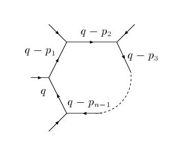
Figure 1: One-loop diagram with $n$ external legs

In Refs. [4], [5] the following relation was derived:

$$(d-\sum_{i=1}^{n}\nu_{i}+1)G_{n-1}I^{(d+2)}_{n}(\{m_{j}^{2}\},\{s_{kl}\})-2\Delta_{n}I^{(d)}_{n}(\{m_{j}^{2}\},\{s_{kl}\})$$

$$~{}~{}~{}~{}=\sum_{k=1}^{n}(\partial_{k}\Delta_{n}){\bf k^{-}}I^{(d)}_{n}(\{m_{j}^{2}\},\{s_{kl}\}),$$ (2.5)

where the operators ${\bf k^{-}}$ shift index of propagators by one unit $\nu_{k}\to\nu_{k}-1$,

$$G_{n-1}=-2^{n}\left|\begin{array}[]{cccc}(p_{1}-p_{n})(p_{1}-p_{n})&(p_{1}-p_{n})(p_{2}-p_{n})&\ldots&(p_{1}-p_{n})(p_{n-1}-p_{n})\\ (p_{1}-p_{n})(p_{2}-p_{n})&(p_{2}-p_{n})(p_{2}-p_{n})&\ldots&(p_{2}-p_{n})(p_{n-1}-p_{n})\\ \vdots&\vdots&\ddots&\vdots\\ (p_{1}-p_{n})(p_{n-1}-p_{n})&(p_{2}-p_{n})(p_{n-1}-p_{n})&\ldots&(p_{n-1}-p_{n})(p_{n-1}-p_{n})\end{array}\right|,$$ (2.6)

$$\Delta_{n}=\left|\begin{array}[]{cccc}Y_{11}&Y_{12}&\ldots&Y_{1n}\\ Y_{12}&Y_{22}&\ldots&Y_{2n}\\ \vdots&\vdots&\ddots&\vdots\\ Y_{1n}&Y_{2n}&\ldots&Y_{nn}\end{array}\right|,$$

$$Y_{ij}=m_{i}^{2}+m_{j}^{2}-s_{ij},~{}~{}~{}~{}~{}~{}~{}~{}~{}~{}~{}~{}~{}~{}~{}s_{ij}=(p_{i}-p_{j})^{2}.$$ (2.7)

Here $p_{i},p_{j}$ are external momenta going through lines $i,j$ respectively, and $m_{j}$ is mass attributed to $j$-th line. Gram determinant $G_{n-1}$ and modified Cayley determinant $\Delta_{n}$ are polynomials depending on scalar products and masses.

It is assumed that these scalar products are made of $d$ dimensional vectors and $G_{n-1}$ and $\Delta_{n}$ are not subject to any restriction or condition specific to some integer values of $d$. Eq. (2.5) is written in the form corresponding to Eq. (2.1). To eliminate integrals with $n$ lines on the left hand - side of Eq. (2.5) the following conditions to be hold:

$$G_{n-1}=0,~{}~{}~{}~{}~{}~{}~{}~{}~{}~{}~{}~{}~{}\Delta_{n}=0.$$ (2.8)

Eq. (2.5) is valid for arbitrary kinematical variables and masses. Solution of Eqs. (2.8) can be easily done with respect to two kinematical variables or masses. Starting from $n=3$ substitution of such solutions into Eq. (2.5) gives nontrivial functional equations.

The method for obtaining functional equations by eliminating complicated integrals from recurrence relations is quite general one. However for multi loop integrals, depending on several kinematical variables, derivation of equations like Eq. (2.5) is computationally challenging. In the next sections we will describe easier and more powerful methods that can be used for deriving functional equations for multi-loop integrals.

3 Deriving functional equations from algebraic relations
between propagators

Setting $\nu_{j}=1$ in Eq. (2.5) and imposing conditions (2.8) leads to the following equation:

$$\sum_{k=1}^{n}(\partial_{k}\Delta_{n}){\bf k^{-}}I^{(d)}_{n}=0.$$ (3.9)

In Eq. (3.9) integrands of ${\bf k^{-}}I^{(d)}_{n}$ are products of $n-1$ propagators depending on different external momenta, i.e. each term in this relation corresponds to the same function but with different arguments. In fact functional equations considered in Refs. [1, 3, 2] are of the same form as Eq. (3.9). The question naturally arises: This relationship holds for integrals or it can be obtained as the consequence of a relationship between integrands?

By inspecting Eq. (3.9), one can suggest the following form of the relation between products of propagators of integrands:

$$\prod_{r=1}^{n}\frac{1}{P_{r}}=\frac{1}{P_{n+1}}\sum_{r=1}^{n}x_{r}{\prod_{\begin{subarray}{c}j=1\\ j\neq r\end{subarray}}^{n}}\left(\frac{1}{P_{j}}\right),$$ (3.10)

where

$$P_{j}=(k_{1}-p_{j})^{2}-m_{j}^{2}+i\epsilon.$$ (3.11)

In what follows we will omit $i\epsilon$ term assuming that all masses have such a correction. Additionally we assume that vectors $p_{j}$ are linearly dependent, i.e. the Gram determinant for the set of vectors $\{p_{j}\}$ is equal to zero. Such a condition is valid for all examples considered in Refs. [1], [2].

Now let’s consider in detail implementation of our prescription for products of 2,3 and 4 propagators. At $n=2$ relation (3.10) reads:

$$\frac{1}{P_{1}P_{2}}=\frac{x_{1}}{P_{2}P_{3}}+\frac{x_{2}}{P_{1}P_{3}},$$ (3.12)

where

$$P_{1}=(k_{1}-p_{1})^{2}-m_{1}^{2},~{}~{}~{}P_{2}=(k_{1}-p_{2})^{2}-m_{2}^{2},~{}~{}~{}P_{3}=(k_{1}-p_{3})^{2}-m_{3}^{2}.$$ (3.13)

According to our assumption three vectors $p_{1}$,$p_{2}$,$p_{3}$ are linearly dependent. Without loss of generality we may assume that

$$p_{3}=y_{31}p_{1}+y_{32}p_{2}.$$ (3.14)

Furthermore, we assume that $k_{1}$ will be integration momentum and scalar quantities $x_{1}$,$x_{2}$, $y_{32}$, $y_{32}$ do not depend on $k_{1}$. Putting all terms in Eq. (3.12) over a common denominator and then equating to zero the coefficients in front of various products of $k_{1}^{2}$, $k_{1}p_{1}$,$k_{1}p_{2}$ yields the following system of equations:

$$y_{32}-x_{2}=0,~{}~{}~{}y_{31}-x_{1}=0,~{}~{}~{}x_{1}+x_{2}=1,$$

$$p_{1}^{2}(x_{1}-y_{31}^{2})+p_{2}^{2}(x_{2}-y_{32}^{2})+y_{31}y_{32}(s_{12}-p_{1}^{2}-p_{2}^{2})-m_{1}^{2}x_{1}-m_{2}^{2}x_{2}+m_{3}^{2}=0.$$ (3.15)

Solution of this system of equations is:

$$x_{1}=y_{31}=\lambda_{2},~{}~{}~{}x_{2}=y_{32}=1-\lambda_{2},$$ (3.16)

where $\lambda_{2}$ is a root of the equation

$$A_{2}\lambda_{2}^{2}+B_{2}\lambda_{2}+C_{2}=0,$$ (3.17)

with

$$A_{2}=s_{12},~{}~{}~{}~{}B_{2}=m_{1}^{2}-m_{2}^{2}-s_{12},~{}~{}~{}~{}C_{2}=m_{2}^{2}-m_{3}^{2}.$$ (3.18)

This solution can be rewritten in an explicit form:

$$x_{1}=y_{31}=\frac{m_{2}^{2}-m_{1}^{2}+s_{12}}{2s_{12}}\pm\frac{\sqrt{\Lambda_{2}+4s_{12}m_{3}^{2}}}{2s_{12}},$$

$$x_{2}=y_{32}=\frac{m_{1}^{2}-m_{2}^{2}+s_{12}}{2s_{12}}\mp\frac{\sqrt{\Lambda_{2}+4s_{12}m_{3}^{2}}}{2s_{12}},$$ (3.19)

where

$$\Lambda_{2}=s_{12}^{2}+m_{1}^{4}+m_{2}^{4}-2s_{12}m_{1}^{2}-2s_{12}m_{2}^{2}-2m_{1}^{2}m_{2}^{2}.$$ (3.20)

Now let’s find algebraic relation for the products of three propagators. At $n=3$ Eq. (3.10) reads:

$$\frac{1}{P_{1}P_{2}P_{3}}=\frac{x_{1}}{P_{4}P_{2}P_{3}}+\frac{x_{2}}{P_{1}P_{4}P_{3}}+\frac{x_{3}}{P_{1}P_{2}P_{4}},$$ (3.21)

where $P_{1}$, $P_{2}$, $P_{3}$ are defined in Eq.(3.13) and

$$P_{4}=(k_{1}-p_{4})^{2}-m_{4}^{2}.$$ (3.22)

In complete analogy with the previous case we can represent one momentum as a combination of other ones. Without loss of generality we may write

$$p_{4}=y_{41}p_{1}+y_{42}p_{2}+y_{43}p_{3},$$ (3.23)

where $y_{ij}$ for the time being are arbitrary coefficients. Putting all terms in Eq. (3.21) over a common denominator and then equating to zero the coefficients in front of various products of $(k_{1}^{2})$, $(k_{1}p_{1})$, $(k_{1}p_{2})$, $(k_{1}p_{3})$ yields the following system of equations:

$$y_{43}-x_{3}=0,~{}~{}~{}~{}~{}y_{42}-x_{2}=0,~{}~{}~{}~{}~{}y_{41}-x_{1}=0,~{}~{}~{}~{}~{}x_{1}+x_{2}+x_{3}=1,$$

$$p_{1}^{2}(x_{1}-y_{41}^{2})+p_{2}^{2}(x_{2}-y_{42}^{2})+p_{3}^{2}(x_{3}-y_{43}^{2})$$

$$+y_{42}y_{43}(s_{23}-p_{2}^{2}-p_{3}^{2})+y_{41}y_{43}(s_{13}-p_{1}^{2}-p_{3}^{2})+y_{41}y_{42}(s_{12}-p_{1}^{2}-p_{2}^{2})$$

$$~{}~{}~{}~{}~{}-m^{2}_{1}x_{1}-m^{2}_{2}x_{2}-m^{2}_{3}x_{3}+m^{2}_{4}=0.$$ (3.24)

Solving these equations for $x_{1}$, $x_{2}$, $x_{3}$, $y_{41}$, $y_{42}$ we have

$$x_{1}=1-\lambda_{3}-y_{43},~{}~{}~{}x_{2}=\lambda_{3},~{}~{}~{}x_{3}=y_{43},~{}~{}~{}y_{41}=1-y_{43}-\lambda_{3},~{}~{}~{}y_{42}=\lambda_{3},$$ (3.25)

where $\lambda_{3}$ is solution of the equation

$$A_{3}\lambda_{3}^{2}+B_{3}\lambda_{3}+C_{3}=0.$$ (3.26)

Here

$$A_{3}=s_{12},$$

$$B_{3}=y_{43}(s_{13}+s_{12}-s_{23})-m_{1}^{2}+m_{2}^{2}-s_{12},$$

$$C_{3}=y_{43}^{2}s_{13}+(m_{3}^{2}-m_{1}^{2}-s_{13})y_{43}+m_{1}^{2}-m_{4}^{2}.$$ (3.27)

Let us now turn to the derivation of algebraic relation for the product of four propagators. At $n=4$ Eq. (3.10) reads:

$$\frac{1}{P_{1}P_{2}P_{3}P_{4}}=\frac{x_{1}}{P_{5}P_{2}P_{3}P_{4}}+\frac{x_{2}}{P_{1}P_{5}P_{3}P_{4}}+\frac{x_{3}}{P_{1}P_{2}P_{5}P_{4}}+\frac{x_{4}}{P_{1}P_{2}P_{3}P_{5}},$$ (3.28)

where $P_{1}$, $P_{2}$, $P_{3}$,$P_{4}$ are defined in Eqs. (3.13), (3.22),

$$P_{5}=(k_{1}-p_{5})^{2}-m_{5}^{2},$$ (3.29)

and $p_{5}$ is a linear combination of vectors $p_{1}$,…,$p_{4}$,

$$p_{5}=y_{51}p_{1}+y_{52}p_{2}+y_{53}p_{3}+y_{54}p_{4}.$$ (3.30)

Putting all terms in Eq. (3.28) over a common denominator and then equating to zero the coefficients in front of different products of $k_{1}^{2}$, $k_{1}p_{j}$ yields system of equations:

$$y_{51}-x_{1}=0,~{}~{}~{}~{}~{}y_{52}-x_{2}=0,~{}~{}~{}~{}~{}y_{53}-x_{3}=0,~{}~{}~{}~{}~{}y_{54}-x_{4}=0,$$

$$x_{1}+x_{2}+x_{3}+x_{4}=1,$$

$$~{}~{}m_{5}^{2}-m_{1}^{2}x_{1}-m_{2}^{2}x_{2}-m_{3}^{2}x_{3}-m_{4}^{2}x_{4}+p_{4}^{2}(x_{4}-y_{54}^{2})$$

$$~{}~{}+p_{3}^{2}(x_{3}-y_{53}^{2})+p_{2}^{2}(x_{2}-y_{52}^{2})+p_{1}^{2}(x_{1}-y_{51}^{2})+(s_{12}-p_{1}^{2}-p_{2}^{2})y_{51}y_{52}$$

$$~{}~{}~{}~{}~{}+(s_{13}-p_{1}^{2}-p_{3}^{2})y_{51}y_{53}+(s_{23}-p_{2}^{2}-p_{3}^{2})y_{52}y_{53}+(s_{14}-p_{1}^{2}-p_{4}^{2})y_{54}y_{51}$$

$$+~{}~{}~{}(s_{24}-p_{2}^{2}-p_{4}^{2})y_{54}y_{52}+(s_{34}-p_{3}^{2}-p_{4}^{2})y_{54}y_{53}=0.$$ (3.31)

Solving this system for $x_{1}$, $x_{2}$, $x_{3}$,$x_{4}$, $y_{51}$, $y_{54}$ we have

$$x_{1}=y_{51}=\lambda_{4},~{}~{}~{}~{}x_{2}=y_{52},~{}~{}~{}~{}x_{3}=y_{53},$$

$$x_{4}=y_{54}=1-x_{1}-x_{2}-x_{3}=1-y_{53}-y_{52}-\lambda_{4},$$ (3.32)

where $\lambda_{4}$ is a solution of the equation

$$A_{4}\lambda_{4}^{2}+B_{4}\lambda_{4}+C_{4}=0,$$ (3.33)

with

$$A_{4}=s_{14},$$

$$B_{4}=(s_{24}-s_{12}+s_{14})y_{52}+(s_{34}-s_{13}+s_{14})y_{53}+m_{1}^{2}-m_{4}^{2}-s_{14},$$

$$C_{4}=s_{24}y_{52}^{2}+(s_{34}-s_{23}+s_{24})y_{52}y_{53}+(m_{2}^{2}-m_{4}^{2}-s_{24})y_{52}+s_{34}y_{53}^{2}$$

$$~{}~{}~{}~{}~{}~{}~{}~{}~{}~{}~{}~{}~{}~{}~{}~{}~{}~{}+(m_{3}^{2}-m_{4}^{2}-s_{34})y_{53}+m_{4}^{2}-m_{5}^{2}.$$ (3.34)

Eqs. (3.21), (3.21) and (3.28) will be used in the next sections to derive functional equations for the propagator, vertex and box type of integrals. Relations between products of five and more propagators can be easily derived in the same way as as it was done for products of two-, three- and four- propagators. From Eq. (3.10) one can derive system of equations and find its solution for arbitrary $n$. Multiplying both sides of Eq. (3.10) by the product of $n+1$ propagators $\prod_{j=1}^{n+1}P_{j}$ yields

$$P_{n+1}=\sum_{r=1}^{n}P_{r},$$ (3.35)

or

$$k_{1}^{2}-2k_{1}p_{n+1}+p_{n+1}^{2}=\sum_{r=1}^{n}x_{r}(k_{1}^{2}-2k_{1}p_{r}+p_{r}^{2}-m_{r}^{2}).$$ (3.36)

Since we assume linear dependence of vectors $p_{r}$, without loss of generality we may write:

$$p_{n+1}=\sum_{j=1}^{n}y_{n+1,j}p_{j}.$$ (3.37)

Substituting (3.37) into Eq.(3.36), collecting terms in front of $k_{1}^{2}$, $k_{1}p_{j}$ and terms without $k_{1}$, equating them to zero after some simplifications yields the following system of $n+2$ equations:

$$x_{k}-y_{n+1,k}=0,~{}~{}~{}~{}~{}k=1,..,n,$$ (3.38)

$$\sum_{k=1}^{n}y_{n+1,k}=1,$$ (3.39)

$$m_{n+1}^{2}-\sum_{k=1}^{n}y_{n+1,k}m_{k}^{2}+\sum_{j=1}^{n}\sum_{l=1}^{j-1}y_{n+1,j}y_{n+1,l}s_{lj}=0.$$ (3.40)

Solving Eq. (3.39) for one of the $y_{ij}$ an substituting this solution into Eq. (3.40) gives quadratic equation for the remaining $y_{ij}$. This quadratic equation can be solved with respect to one of the parameters $y_{ij}$. Thus the solution of the system of equations (3.38), (3.39), (3.40) will depend on $n-2$ arbitrary parameters $y_{ij}$ and one arbitrary mass $m_{n}$.

It is interesting to note that for any $n$, functional equations for integrals with all masses equal to zero and functional equations for integrals with all masses equal are the same. In case of equal masses, two mass dependent terms in Eq. (3.40) cancel each other due to Eq. (3.39). In both cases systems of equations for $x_{i}$, $y_{jk}$ are the same and therefore arguments of integrals are the same.

Eq. (3.12) is analogous to the equation for splitting propagators presented in Ref. [6]. Eq. (3.21) is a generalization of Eq. (3.12). Indeed, setting $y_{43}=x_{3}=0$, canceling common factor $P_{3}$ on both sides of Eq. (3.21) yields relation similar to (3.12). In turn Eq. (3.28) is a generalization of (3.21).

3.1 Prototypes of functional equations

Multiplying algebraic relations (3.12),(3.21), (3.28) by products of any number of propagators raised to arbitrary powers $\nu_{j}$

$$\prod_{j=n_{0}}^{N}\frac{1}{[(k_{1}-p_{j})-m_{j}^{2}]^{\nu_{j}}}$$ (3.41)

and integrating with respect to $k_{1}$ we get a functional equation for one-loop integrals. Eqs.  (3.12), (3.21), (3.28) also can be used to derive functional equations for integrals with any number of loops. Multiplying algebraic relations for propagators by function corresponding to Feynman integral depending on momentum $k_{1}$ and any number of external momenta and then integrating with respect to $k_{1}$ will produce functional equations. Just for demonstrational purposes we present graphically in Figure 2 functional equation based on $n$ propagator relation.

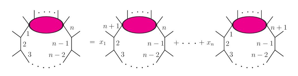
Figure 2: $n$ - propagator functional equation

The blob on this picture correspond to either product of propagators raised to arbitrary powers or to an integral with any number of loops and external legs. One of the external momenta of this multi loop integral should be $k_{1}$.

4 Some examples of functional equations

In this section several particular examples of functional equations resulting from algebraic relations for products of propagators will be considered.

4.1 Functional equation for the one-loop propagator type integral

First, we consider the simplest case, namely, functional equation for the integral $I^{(d)}_{2}$:

$$I_{2}^{(d)}(m_{j}^{2},m_{k}^{2};~{}s_{jk})=\int\frac{d^{d}k_{1}}{i\pi^{{d}/{2}}}\frac{1}{[(k_{1}-p_{j})^{2}-m_{j}^{2}][(k_{1}-p_{k})^{2}-m_{k}^{2}]}.$$ (4.42)

Integrating both sides of Eq. (3.12) with respect to $k_{1}$, we get:

$$I_{2}^{(d)}(m_{1}^{2},m_{2}^{2},s_{12})=x_{1}I_{2}^{(d)}(m_{2}^{2},m_{3}^{2},s_{23})+x_{2}I_{2}^{(d)}(m_{1}^{2},m_{3}^{2},s_{13}).$$ (4.43)

The arguments $s_{13}$, $s_{23}$ of integrals on the right hand - side depend on $y_{31}$, $y_{32}$

$$s_{13}=(p_{1}-p_{3})^{2}=(y_{31}-1)^{2}p_{1}^{2}+2y_{32}(y_{31}-1)p_{1}p_{2}+y_{32}^{2}p_{2}^{2},$$

$$s_{23}=(p_{2}-p_{3})^{2}=p_{1}^{2}y_{31}^{2}+2(y_{32}-1)y_{31}p_{1}p_{2}+(y_{32}-1)^{2}p_{2}^{2}.$$ (4.44)

Substituting solution for $y_{ij}$ from Eq. (3.16) into Eq. (4.44) yields:

$$s_{13}=\frac{m_{2}^{4}-2m_{2}^{2}m_{1}^{2}-2m_{2}^{2}s_{12}+m_{1}^{4}+s_{12}^{2}+2s_{12}m_{3}^{2}}{2s_{12}}$$

$$~{}~{}~{}~{}~{}~{}~{}~{}~{}~{}~{}~{}~{}~{}~{}~{}~{}~{}~{}~{}~{}~{}~{}~{}~{}~{}~{}~{}~{}~{}~{}\pm\frac{m_{1}^{2}-m_{2}^{2}+s_{12}}{2s_{12}}\sqrt{\Lambda_{2}+4s_{12}m_{3}^{2}}$$

$$s_{23}=\frac{s_{12}^{2}-2m_{1}^{2}s_{12}+m_{1}^{4}+m_{2}^{4}-2m_{1}^{2}m_{2}^{2}+2s_{12}m_{3}^{2}}{2s_{12}}$$

$$~{}~{}~{}~{}~{}~{}~{}~{}~{}~{}~{}~{}~{}~{}~{}~{}~{}~{}~{}~{}~{}~{}~{}~{}~{}~{}~{}~{}~{}~{}~{}\pm\frac{m_{1}^{2}-m_{2}^{2}-s_{12}}{2s_{12}}\sqrt{\Lambda_{2}+4s_{12}m_{3}^{2}}.$$ (4.45)

In this equation $m_{3}^{2}$ is an arbitrary parameter and can be taken at will. Functional equation (4.43) is in agreement with the result presented in Refs. [1],[2].

4.2 Functional equations for the one-loop vertex type integral

Functional equations for the vertex type integral

$$I_{3}^{(d)}(m_{1}^{2},m_{2}^{2},m_{3}^{2},s_{23},s_{13},s_{12})$$

$$~{}~{}~{}~{}~{}~{}~{}~{}~{}~{}=\int\frac{d^{d}k_{1}}{i\pi^{{d}/{2}}}\frac{1}{[(k_{1}-p_{1})^{2}-m_{1}^{2}][(k_{1}-p_{2})^{2}-m_{2}^{2}][(k_{1}-p_{3})^{2}-m_{3}^{2}]},$$ (4.46)

can be obtained from Eq. (3.12) as well as from Eq. (3.21). Multiplying Eq. (3.12) with the factor ${1}/{P_{4}}$ where

$$P_{4}={(k_{1}-p_{4})^{2}-m_{4}^{2}},$$ (4.47)

and integrating over $k_{1}$ leads to the equation:

$$\int\frac{d^{d}k_{1}}{P_{1}P_{2}P_{4}}=x_{1}\int\frac{d^{d}k_{1}}{P_{2}P_{3}P_{4}}+x_{2}\int\frac{d^{d}k_{1}}{P_{1}P_{3}P_{4}}.$$ (4.48)

This equation in terms of integrals $I_{3}^{(d)}$ reads

$$I_{3}^{(d)}(m_{1}^{2},m_{2}^{2},m_{4}^{2};s_{24},s_{14},s_{12})$$

$$~{}~{}~{}~{}~{}~{}~{}=x_{1}I_{3}^{(d)}(m_{2}^{2},m_{3}^{2},m_{4}^{2};s_{34},s_{24},s_{23})+x_{2}I_{3}^{(d)}(m_{1}^{2},m_{3}^{2},m_{4}^{2};s_{34},s_{14},s_{13}).$$ (4.49)

Two more functional equations can be obtained from Eq. (4.48) by symmetric permutations $(m_{1},p_{1})\leftrightarrow(m_{4},p_{4})$ and $(m_{2},p_{2})\leftrightarrow(m_{4},p_{4})$.

Another functional equation for the vertex type integral can be obtained by integrating Eq. (3.21) with respect to $k_{1}$:

$$I_{3}^{(d)}(m_{1}^{2},m_{2}^{2},m_{3}^{2},s_{23},s_{13},s_{12})=(1-\lambda_{3}-y_{43})I_{3}^{(d)}(m^{2}_{4},m_{2}^{2},m_{3}^{2},s_{23},s_{34},{s}_{24})$$

$$~{}~{}~{}~{}~{}+\lambda_{3}I_{3}^{(d)}(m_{1}^{2},m_{4}^{2},m_{3}^{2},{s}_{34},{s}_{13},s_{14})+y_{43}I_{3}^{(d)}(m_{1}^{2},m_{2}^{2},m_{4}^{2},s_{24},{s}_{14},{s}_{13}),$$ (4.50)

where

$${s}_{14}=(m^{2}_{1}-m^{2}_{2}+s_{12})\lambda_{3}+(m^{2}_{1}-m^{2}_{3}+s_{13})y_{43}+m^{2}_{4}-m^{2}_{1},$$

$${s}_{24}=(m^{2}_{1}-s_{12}-m^{2}_{2})\lambda_{3}+(m_{1}^{2}-m_{3}^{2}-s_{12}+s_{23})y_{43}+m^{2}_{4}-m^{2}_{1}+s_{12},$$

$${s}_{34}=(m^{2}_{1}-s_{13}+s_{23}-m^{2}_{2})\lambda_{3}+(m^{2}_{1}-m^{2}_{3}-s_{13})y_{43}+m^{2}_{4}-m^{2}_{1}+s_{13}.$$ (4.51)

There is an essential difference between functional equation Eq. (4.49) obtained from Eq. (3.12) and functional equation (4.50) derived from Eq. (3.21). For example, at $m_{1}^{2}=m_{2}^{2}=m_{3}^{2}=m_{4}^{2}=0$, Eq. (4.49) becomes trivial while from Eq. (4.50) for the integral

$$I_{3}^{(d)}(0,0,0,s_{23},s_{13},s_{12})\equiv I_{3}^{(d)}(s_{23},s_{13},s_{12})$$ (4.52)

we obtain nontrivial functional equation:

$$I^{(d)}_{3}(s_{23},s_{13},s_{12})$$

$$=(1-\lambda_{3}-y_{43})I^{(d)}_{3}(s_{12}(1-\lambda_{3}-y_{43})+s_{23}y_{43},s_{23},\lambda_{3}(s_{23}-s_{13})+s_{13}(1-y_{43}))$$

$$+\lambda_{3}I^{(d)}_{3}(s_{13}y_{43}+\lambda_{3}s_{12},\lambda_{3}(s_{23}-s_{13})+s_{13}(1-y_{43}),s_{13})$$

$$+y_{43}I^{(d)}_{3}(s_{12},s_{12}(1-\lambda_{3}-y_{43})+s_{23}y_{43},s_{13}y_{43}+\lambda_{3}s_{12}),$$ (4.53)

where $\lambda_{3}$ is a root of the quadratic equation

$$s_{12}\lambda_{3}^{2}-(s_{12}-s_{12}y_{43}-s_{13}y_{43}+s_{23}y_{43})\lambda_{3}+y_{43}^{2}s_{13}-y_{43}s_{13}=0.$$ (4.54)

If one argument of $I_{3}^{(d)}(s_{23},s_{13},s_{12})$ is zero then by applying functional equation (4.53) such an integral can be expressed in terms of integrals $I_{3}^{(d)}$ with two arguments equal to zero. For example, at $s_{23}=0$ and $y_{43}=s_{12}/(s_{12}-s_{13})$ the relation (4.53) becomes:

$$I_{3}^{(d)}(0,s_{13},s_{12})=\frac{s_{12}}{s_{12}-s_{13}}I_{3}^{(d)}(s_{12},0,0)-\frac{s_{13}}{s_{12}-s_{13}}I_{3}^{(d)}(0,0,s_{13}).$$ (4.55)

This is a typical example how functional equations can be used to simplify evaluation of an integral by reducing it to a combination of integrals with fewer number of arguments.

At $m_{1}^{2}=m_{2}^{2}=m_{3}^{2}=m_{4}^{2}=m^{2}$, similar to the previous case, Eq.(4.49) degenerate while from Eq.(4.50) for the integral

$$I_{3}^{(d)}(m^{2},m^{2},m^{2},s_{23},s_{13},s_{12})\equiv I_{3}^{(d)}(m^{2};s_{23},s_{13},s_{12})$$ (4.56)

we obtain nontrivial functional equation:

$$I^{(d)}_{3}(m^{2};s_{23},s_{13},s_{12})$$

$$=(1-\lambda_{3}-y_{43})I^{(d)}_{3}(m^{2};s_{12}(1-\lambda_{3}-y_{43})+s_{23}y_{43},s_{23},\lambda_{3}(s_{23}-s_{13})+s_{13}(1-y_{43}))$$

$$+\lambda_{3}I^{(d)}_{3}(m^{2};s_{13}y_{43}+\lambda_{3}s_{12},\lambda_{3}(s_{23}-s_{13})+s_{13}(1-y_{43}),s_{13})$$

$$+y_{43}I^{(d)}_{3}(m^{2};s_{12},s_{12}(1-\lambda_{3}-y_{43})+s_{23}y_{43},s_{13}y_{43}+\lambda_{3}s_{12}),$$ (4.57)

where $\lambda_{3}$ is a root of the quadratic equation

$$s_{12}\lambda_{3}^{2}-(s_{12}-s_{12}y_{43}-s_{13}y_{43}+s_{23}y_{43})\lambda_{3}+y_{43}^{2}s_{13}-y_{43}s_{13}=0.$$ (4.58)

Eqs. (4.57), (4.58) are identical to Eqs. (4.53),(4.54) respectively and therefore functional equation for the integral with massless propagators and functional equation for the integral with all masses equal are the same. Eq. (4.57) at $s_{23}=0$ and $y_{43}=s_{12}/(s_{12}-s_{13})$ leads to the relation similar to (4.55):

$$I_{3}^{(d)}(m^{2};0,s_{13},s_{12})=\frac{s_{12}}{s_{12}-s_{13}}I_{3}^{(d)}(m^{2};s_{12},0,0)-\frac{s_{13}}{s_{12}-s_{13}}I_{3}^{(d)}(m^{2};0,0,s_{13}).$$ (4.59)

This is not surprising because coefficients of the Eq. (4.57) are mass independent and in the integrand $m^{2}$ and $i\epsilon$ appear in the covariant combination $m^{2}-i\epsilon$. For this reason the similarity of functional equations for massless integrals and integrals with all masses equal take place for integrals with more external legs and more loops.

4.3 Functional equations for one-loop box type integrals

Functional equations for the box type integrals can be obtained by multiplying relation (3.12) by two propagators, or by multiplying relation (3.21) by one propagator and then integrating over momentum $k_{1}$. Yet another relation can be obtained just by integrating Eq. (3.28) over momentum $k_{1}$:

$$I_{4}^{(d)}(m_{1}^{2},m_{2}^{2},m_{3}^{2},m_{4}^{2};s_{12},s_{23},s_{34},s_{14},s_{24},s_{13})$$

$$~{}~{}~{}~{}~{}~{}~{}~{}~{}~{}~{}~{}~{}~{}~{}~{}~{}~{}~{}~{}=\lambda_{4}I_{4}^{(d)}(m_{5}^{2},m_{2}^{2},m_{3}^{2},m_{4}^{2};s_{25},s_{23},s_{34},s_{45},s_{24},s_{35})$$

$$~{}~{}~{}~{}~{}~{}~{}~{}~{}~{}~{}~{}~{}~{}~{}~{}~{}~{}~{}~{}+y_{52}I_{4}^{(d)}(m_{1}^{2},m_{5}^{2},m_{3}^{2},m_{4}^{2};s_{15},s_{35},s_{34},s_{14},s_{45},s_{13})$$

$$~{}~{}~{}~{}~{}~{}~{}~{}~{}~{}~{}~{}~{}~{}~{}~{}~{}~{}~{}~{}+y_{53}I_{4}^{(d)}(m_{1}^{2},m_{2}^{2},m_{5}^{2},m_{4}^{2};s_{12},s_{25},s_{45},s_{14},s_{24},s_{15})$$

$$+(1-y_{52}-y_{53}-\lambda_{4})I_{4}^{(d)}(m_{1}^{2},m_{2}^{2},m_{3}^{2},m_{5}^{2};s_{12},s_{23},s_{35},s_{15},s_{25},s_{13}).$$ (4.60)

Here $\lambda_{4}$ is defined in Eq. (3.33) and $m_{5}$,$y_{52}$, $y_{53}$ are arbitrary parameters and

$$s_{15}=\lambda_{4}(m_{4}^{2}-s_{14}-m_{1}^{2})+y_{53}(m_{4}^{2}-m_{3}^{2}-s_{14}+s_{13})+y_{52}(m_{4}^{2}-m_{2}^{2}-s_{14}+s_{12})$$

$$~{}~{}~{}~{}~{}~{}~{}~{}~{}~{}~{}~{}~{}~{}~{}~{}~{}~{}~{}~{}~{}~{}~{}~{}~{}~{}~{}~{}~{}~{}~{}~{}~{}~{}~{}~{}~{}~{}~{}~{}~{}~{}~{}~{}~{}~{}~{}~{}~{}~{}+s_{14}+m_{5}^{2}-m_{4}^{2},$$

$$s_{25}=\lambda_{4}(m_{4}^{2}-m_{1}^{2}-s_{24}+s_{12})+y_{53}(m_{4}^{2}-m_{3}^{2}-s_{24}+s_{23})+y_{52}(m_{4}^{2}-m_{2}^{2}-s_{24})$$

$$~{}~{}~{}~{}~{}~{}~{}~{}~{}~{}~{}~{}~{}~{}~{}~{}~{}~{}~{}~{}~{}~{}~{}~{}~{}~{}~{}~{}~{}~{}~{}~{}~{}~{}~{}~{}~{}~{}~{}~{}~{}~{}~{}~{}~{}~{}~{}~{}~{}~{}+s_{24}+m_{5}^{2}-m_{4}^{2},$$

$$s_{35}=\lambda_{4}(m_{4}^{2}-m_{1}^{2}-s_{34}+s_{13})+y_{53}(m_{4}^{2}-m_{3}^{2}-s_{34})+y_{52}(m_{4}^{2}-m_{2}^{2}-s_{34}+s_{23})$$

$$~{}~{}~{}~{}~{}~{}~{}~{}~{}~{}~{}~{}~{}~{}~{}~{}~{}~{}~{}~{}~{}~{}~{}~{}~{}~{}~{}~{}~{}~{}~{}~{}~{}~{}~{}~{}~{}~{}~{}~{}~{}~{}~{}~{}~{}~{}~{}~{}~{}~{}+s_{34}+m_{5}^{2}-m_{4}^{2},$$

$$s_{45}=\lambda_{4}(s_{14}+m_{4}^{2}-m_{1}^{2})+y_{53}(s_{34}+m_{4}^{2}-m_{3}^{2})+y_{52}(s_{24}+m_{4}^{2}-m_{2}^{2})$$

$$~{}~{}~{}~{}~{}~{}~{}~{}~{}~{}~{}~{}~{}~{}~{}~{}~{}~{}~{}~{}~{}~{}~{}~{}~{}~{}~{}~{}~{}~{}~{}~{}~{}~{}~{}~{}~{}~{}~{}~{}~{}~{}~{}~{}~{}~{}~{}~{}~{}~{}+m_{5}^{2}-m_{4}^{2}.$$ (4.61)

Arbitrary parameters in this functional equation can be chosen from the requirement of simplicity of evaluation of integrals on the right hand - side of Eq. (4.60) or from some other requirements. For example, one can choose these parameters by transforming arguments to a certain kinematical region needed for analytic continuation of the original integral.

4.4 Functional equation for two-loop vertex type integral

The method described in the previous section can be applied to multi loop integrals. Consider, for example, integral corresponding to the diagram given in Figure 3.

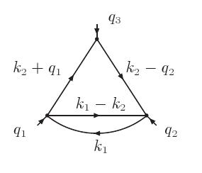
Figure 3: Diagram corresponding to $R(m_{1}^{2},m_{2}^{2},m_{3}^{2},m_{4}^{2};~{}q_{1}^{2},q_{2}^{2},q_{3}^{2})$

If we multiply Eq. (3.12) by the one-loop integral depending on $k_{1}$

$$\int\frac{d^{d}k_{2}}{[k_{2}^{2}-m_{4}^{2}][(k_{1}-k_{2})^{2}-m_{5}^{2}]}$$ (4.62)

and integrate with respect to momentum $k_{1}$ then we obtain functional equation

$$R(m_{1}^{2},m_{2}^{2},m_{3}^{2},m_{4}^{2};~{}q_{1}^{2},q_{2}^{2},q_{3}^{2})$$

$$~{}~{}~{}~{}~{}~{}~{}~{}~{}~{}~{}~{}~{}=\alpha R(0,m_{2}^{2},m_{3}^{2},m_{4}^{2};~{}Q^{2},q_{2}^{2},(m_{2}^{2}-m_{1}^{2}+q_{3}^{2})\alpha-m_{2}^{2})$$

$$~{}~{}~{}~{}~{}~{}~{}~{}~{}~{}~{}~{}~{}+(1-\alpha)R(m_{1}^{2},0,m_{3}^{2},m_{4}^{2};~{}q_{1}^{2},Q^{2},(m_{2}^{2}-m_{1}^{2}-q_{3}^{2})\alpha+q_{3}^{2}-m_{2}^{2}),$$ (4.63)

where

$$R(m_{1}^{2},m_{2}^{2},m_{3}^{2},m_{4}^{2};~{}q_{1}^{2},q_{2}^{2},q_{3}^{2})$$

$$=\int\int\frac{d^{d}k_{1}d^{d}k_{2}}{(i\pi^{d/2})^{2}}\frac{1}{[(k_{2}+q_{1})^{2}-m_{1}^{2}][(k_{2}-q_{2})^{2}-m_{2}^{2}][k_{1}^{2}-m_{3}^{2}][(k_{1}-k_{2})^{2}-m_{4}^{2}]},$$ (4.64)

$$Q^{2}=(q_{1}^{2}-q_{2}^{2}-m_{1}^{2}+m_{2}^{2})\alpha+q_{2}^{2}-m_{2}^{2},$$ (4.65)

$$\alpha=\frac{q_{3}^{2}-m_{1}^{2}+m_{2}^{2}\pm\sqrt{\Delta}}{2q_{3}^{2}},$$ (4.66)

$$\Delta=q_{3}^{4}+m_{1}^{4}+m_{2}^{4}-2q_{3}^{2}m_{1}^{2}-2q_{3}^{2}m_{2}^{2}-2m_{1}^{2}m_{2}^{2}.$$ (4.67)

Integrals of this type arise, for example, in calculations of two-loop radiative corrections in the electroweak theory. Instead of the integral $R(m_{1}^{2},m_{2}^{2},m_{3}^{2},m_{4}^{2};~{}q_{1}^{2},q_{2}^{2},q_{3}^{2})$ one can consider derivative of $R$ with respect to $m_{3}^{2}$ which is UV finite:

$$\frac{\partial R}{\partial m_{3}^{2}}\equiv R_{3}(m_{1}^{2},m_{2}^{2},m_{3}^{2},m_{4}^{2};~{}q_{1}^{2},q_{2}^{2},q_{3}^{2})$$

$$=\int\int\frac{d^{d}k_{1}d^{d}k_{2}}{(i\pi^{d/2})^{2}}\frac{1}{[(k_{2}+q_{1})^{2}-m_{1}^{2}][(k_{2}-q_{2})^{2}-m_{2}^{2}][k_{1}^{2}-m_{3}^{2}]^{2}[(k_{1}-k_{2})^{2}-m_{4}^{2}]}.$$ (4.68)

Integral $R_{3}$ satisfy the following functional equations:

$$R_{3}(m_{1}^{2},m_{2}^{2},m_{3}^{2},m_{4}^{2};~{}q_{1}^{2},q_{2}^{2},q_{3}^{2})$$

$$~{}~{}~{}~{}~{}~{}~{}~{}~{}~{}~{}~{}~{}=\alpha R_{3}(0,m_{2}^{2},m_{3}^{2},m_{4}^{2};~{}Q^{2},q_{2}^{2},(m_{2}^{2}-m_{1}^{2}+q_{3}^{2})\alpha-m_{2}^{2})$$

$$~{}~{}~{}~{}~{}~{}~{}~{}~{}~{}~{}~{}~{}+(1-\alpha)R_{3}(m_{1}^{2},0,m_{3}^{2},m_{4}^{2};~{}q_{1}^{2},Q^{2},(m_{2}^{2}-m_{1}^{2}-q_{3}^{2})\alpha+q_{3}^{2}-m_{2}^{2}).$$ (4.69)

This relation can be used for computing basis integral arising in calculation of two-loop radiative correction to the ortho -positronium lifetime. In particular one of these basis integrals corresponds to kinematics $m_{1}^{2}=m_{2}^{2}=m_{3}^{2}=m_{4}^{2}=m^{2}$, $q_{1}^{2}=q_{2}^{2}=m^{2}$, $q_{3}^{2}=4m^{2}$. In this case relation (4.69) reads

$$R_{3}(m^{2},m^{2},m^{2},m^{2};~{}m^{2},m^{2},4m^{2})=R_{3}(0,m^{2},m^{2},m^{2};0,m^{2},m^{2}).$$ (4.70)

Integral on the right hand-side is in fact propagator type integral with one massless line. Applying recurrence relations given in Ref. [7] this integral can be reduced to simpler integral:

$$R_{3}(0,m^{2},m^{2},m^{2};0,m^{2},m^{2})$$

$$=\frac{1}{(i\pi^{d/2})^{2}}\int\int\frac{d^{d}k_{1}d^{d}k_{2}}{k_{1}^{2}(k_{2}^{2}-m^{2})[(k_{1}-k_{2})^{2}-m^{2}]^{2}[(k_{1}+q_{1})^{2}-m^{2}]}$$

$$=\frac{2}{3(d-3)}J_{111}^{(d-2)}(m^{2}),$$ (4.71)

where

$$J_{111}^{(d)}(q^{2})=\frac{1}{(i\pi^{d/2})^{2}}\int\int\frac{d^{d}k_{1}d^{d}k_{2}}{(k_{1}^{2}-m^{2})[(k_{1}-k_{2})^{2}-m^{2}][(k_{2}-q)^{2}-m^{2}]}.$$ (4.72)

At $q^{2}=m^{2}$, the result for $J_{111}^{(d)}(q^{2})$ is known [8]:

$$\frac{m^{6-2d}}{8}(d-4)^{2}(d-2)(d-3)J_{111}^{(d)}(m^{2})$$

$$~{}~{}~{}~{}~{}~{}~{}=\,{}_{3}F_{2}\!\!\left[\begin{array}[]{c}1,3-d,\frac{1}{2}\,;\\ \frac{5-d}{2},\frac{d}{2}\,;\end{array}1\right]+(d-3)\,{}_{3}F_{2}\!\!\left[\begin{array}[]{c}1,\frac{4-d}{2},\frac{d-1}{2}\,;\\ \frac{3}{2},d-1\,;\end{array}1\right],$$ (4.77)

and it can be used for the $\varepsilon$ expansion of $R$ and $R_{3}$. As was already mentioned at $q_{1}^{2}=q_{2}^{2}=m^{2}$, $q_{3}^{2}=4m^{2}$ integrals on the right hand - side of Eq.(4.63) correspond to propagator type integrals. Analytic result for $R$ reads

$$(d-3)R(m^{2},m^{2},m^{2},m^{2},m^{2},m^{2},4m^{2})$$

$$~{}~{}~{}~{}~{}~{}~{}~{}~{}~{}~{}=\frac{1}{8m^{4}(d-4)}\left[2m^{2}(3d-8)(d-3)J_{111}^{(d)}-3(d-2)^{2}\left(T_{1}^{(d)}\right)^{2}\right],$$ (4.78)

where

$$T_{1}^{(d)}=-{\Gamma\left(1-\frac{d}{2}\right)}(m^{2})^{(d-2)/2}.$$ (4.79)

We checked that several first terms in the $\varepsilon=(4-d)/2$ expansion of $R$ and $R_{3}$ are in agreement with results of [9]. The main profit from functional equations for $R$ and $R_{3}$ comes from the fact that vertex integrals were expressed in terms of simpler, propagator type integrals.

5 Deriving functional equation by deforming propagators

The method described in the previous section does not work for deriving functional equations for all kinds of Feynman integrals. For example, we did not found functional equation for the two-loop vacuum type integral given in Figure 4.

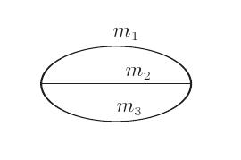
Figure 4: Two-loop vacuum type diagram

In this section we shall describe another method that extends the class of integrals for which we can obtain functional equations. The method is based on transformation of functional equations for some auxiliary integrals depending on arbitrary parameters into functional equations for integrals of interest. Such functional equations will be derived from algebraic relations for ‘deformed propagators’ which will be defined in the next section. These auxiliary integrals will be transformed into $\alpha$ parametric representation. In general characteristic polynomials of these integrals in $\alpha$ parametric representation differ from those for the investigated integral. Functional equation for the integral of interest can be obtained in case when it will be possible to map characteristic polynomials of auxiliary integrals with ‘deformed propagators’ to characteristic polynomials of this integral. Such a mapping will be performed by rescaling $\alpha$ parameters and appropriate choice of arbitrary ‘deforming parameters’.

5.1 Algebraic relations for products of deformed propagators

In the previous section to derive functional equation we added to our consideration a propagator with combination of external momenta taken with arbitrary scalar coefficient. Now we consider generalization of this method.

To find functional equation for $L$-loop Feynman integral depending on $E$- external momenta we start from the relation of the form

$$\prod_{r=1}^{n}\frac{1}{D_{r}}=\frac{1}{D_{n+1}}\sum_{r=1}^{n}x_{r}{\prod_{\begin{subarray}{c}j=1\\ j\neq r\end{subarray}}^{n}}\left(\frac{1}{D_{j}}\right),$$ (5.80)

where $D_{j}$ is defined as:

$$D_{j}=Q_{j}^{2}-m_{j}^{2}+i\epsilon,$$ (5.81)

with

$$Q_{j}=\sum_{l=1}^{L}a^{(j)}_{jl}k_{l}+\sum_{l=1}^{E+1}b^{(j)}_{jl}p_{l},$$ (5.82)

and $a^{(j)}_{jl}$, $b^{(j)}_{jl}$ for the time being are arbitrary scalar parameters. Some of these parameters as well as $x_{r}$ will be fixed from the equation (5.80). Another part of these parameters will be fixed from the requirement that the product of propagators in (5.80) should correspond to the integrand of the integral with the considered topology. We would like to remark that instead of deformation of propagators proposed in Eqs. (5.81),(5.82) one can use other deformations. For example, all terms in denominators of propagators can be taken with arbitrary scalar coefficients:

$$Q_{j}^{2}=\sum_{l,r=1}^{L}a^{(j)}_{rl}(k_{r}\cdot k_{l})+\sum_{l=1}^{L}\sum_{r=1}^{E+1}b^{(j)}_{rl}(p_{r}\cdot k_{l})+\sum_{r,l=1}^{E+1}c^{(j)}_{rl}(p_{r}\cdot p_{l}).$$ (5.83)

To establish algebraic relation (5.80) we put all terms over a common denominator and then equate coefficients in front scalar products depending on integration momenta. Solving obtained system of equations gives some restrictions on the scalar parameters.

In general integrals obtained by integrating products of ‘deformed propagators’ will not correspond to usual Feynman integrals. Further restrictions on parameters should be imposed in order to obtain relations between integrals corresponding to Feynman integrals coming from a realistic quantum field theory models.

5.2 Functional equation for two-loop vacuum type integral with arbitrary masses

As an example, let us consider derivation of functional equation for the two-loop vacuum type integral given in Figure 4:

$$J_{0}^{(d)}(m_{1}^{2},m_{2}^{2},m_{3}^{2})=\int\!\!\int\frac{{\rm d}^{d}k_{1}{\rm d}^{d}k_{2}}{(i\pi^{d/2})^{2}}\frac{1}{(k_{1}^{2}-m_{1}^{2})((k_{1}-k_{2})^{2}-m_{2}^{2})(k_{2}^{2}-m_{3}^{2})}.$$ (5.84)

Analytic expression for this integral was presented in Ref [10]. Instead of this integral we will first consider an auxiliary integral with integrand made from ‘deformed propagators’ defined in Eqs.(5.81), (5.82):

$$\widetilde{J}_{0}^{(d)}(m_{1}^{2},m_{2}^{2},m_{3}^{2})=\int\!\!\int\frac{{\rm d}^{d}k_{1}{\rm d}^{d}k_{2}}{(i\pi^{d/2})^{2}}\frac{1}{D_{1}D_{2}D_{3}},$$ (5.85)

where

$$D_{1}=(a_{1}k_{1}+a_{2}k_{2})^{2}-m_{1}^{2}+i\epsilon,~{}~{}D_{2}=(b_{1}k_{1}+b_{2}k_{2})^{2}-m_{2}^{2}+i\epsilon,$$

$$D_{3}=(h_{1}k_{1}+h_{2}k_{2})^{2}-m_{3}^{2}+i\epsilon.~{}~{}$$ (5.86)

For the product of three deformed propagators one can try to find an algebraic relation of the form:

$$\frac{1}{D_{1}D_{2}D_{3}}=\frac{x_{1}}{D_{4}D_{2}D_{3}}+\frac{x_{2}}{D_{1}D_{4}D_{3}}+\frac{x_{3}}{D_{1}D_{2}D_{4}},$$ (5.87)

where $D_{1}$, $D_{2}$,$D_{3}$ are defined in Eq.(5.86) and

$$D_{4}=(r_{1}k_{1}+r_{2}k_{2})^{2}-m_{4}^{2}.$$ (5.88)

Here $m_{k}$ are arbitrary masses, $x_{k}$, $a_{j}$, $b_{i}$, $h_{s}$, $r_{l}$ are undetermined parameters and $k_{1}$, $k_{2}$ will be integration momenta.

Putting in Eq. (5.87) all over a common denominator and equating to zero coefficients in front of different products of $k_{1}^{2}$, $k_{2}^{2}$ and $k_{1}k_{2}$ leads to the system of equations:

$$r_{1}^{2}-x_{1}a_{1}^{2}-x_{2}b_{1}^{2}-x_{3}h_{1}^{2}=0,~{}~{}~{}r_{1}r_{2}-x_{1}a_{1}a_{2}-x_{2}b_{1}b_{2}-x_{3}h_{1}h_{2}=0,$$

$$r_{2}^{2}-x_{1}a_{2}^{2}-x_{2}b_{2}^{2}-x_{3}h_{2}^{2}=0,~{}~{}~{}~{}m_{4}^{2}-x_{1}m_{1}^{2}-x_{2}m_{2}^{2}-x_{3}m_{3}^{2}=0.$$ (5.89)

Solving this system for $r_{1}$, $x_{1}$, $x_{2}$, $x_{3}$ we have:

$$r_{1}=r_{2}\lambda,$$

$$Ax_{1}=r_{2}^{2}(h_{1}h_{2}m_{2}^{2}-b_{2}b_{1}m_{3}^{2})+b_{2}h_{2}(b_{1}h_{2}-b_{2}h_{1})m_{4}^{2}-r_{2}^{2}(h_{2}^{2}m_{2}^{2}-m_{3}^{2}b_{2}^{2})~{}\lambda,$$

$$Ax_{2}=-r_{2}^{2}(m_{1}^{2}h_{2}h_{1}-a_{2}a_{1}m_{3}^{2})-a_{2}h_{2}(a_{1}h_{2}-a_{2}h_{1})m_{4}^{2}+r_{2}^{2}(h_{2}^{2}m_{1}^{2}-m_{3}^{2}a_{2}^{2})~{}\lambda,$$

$$Ax_{3}=r_{2}^{2}(m_{1}^{2}b_{2}b_{1}-a_{2}a_{1}m_{2}^{2})+a_{2}b_{2}(a_{1}b_{2}-a_{2}b_{1})m_{4}^{2}-r_{2}^{2}(b_{2}^{2}m_{1}^{2}-m_{2}^{2}a_{2}^{2})~{}\lambda,$$ (5.90)

where $\lambda$ is a root of the quadratic equation

$$A\lambda^{2}+B\lambda+C=0,$$ (5.91)

and

$$A=b_{2}h_{2}(b_{1}h_{2}-h_{1}b_{2})m_{1}^{2}+a_{2}h_{2}(h_{1}a_{2}-a_{1}h_{2})m_{2}^{2}+a_{2}b_{2}(a_{1}b_{2}-b_{1}a_{2})m_{3}^{2},$$

$$B=(h_{1}b_{2}-b_{1}h_{2})(b_{1}h_{2}+h_{1}b_{2})m_{1}^{2}+(a_{1}h_{2}-h_{1}a_{2})(a_{1}h_{2}+h_{1}a_{2})m_{2}^{2}$$

$$~{}~{}~{}~{}~{}~{}~{}~{}~{}~{}~{}~{}~{}~{}~{}~{}~{}~{}~{}~{}~{}~{}~{}~{}~{}~{}~{}~{}~{}~{}~{}~{}~{}~{}~{}~{}~{}~{}~{}+(b_{1}a_{2}-a_{1}b_{2})(a_{1}b_{2}+b_{1}a_{2})m_{3}^{2},$$

$$C=b_{1}h_{1}(b_{1}h_{2}-h_{1}b_{2})m_{1}^{2}+a_{1}h_{1}(a_{2}h_{1}-a_{1}h_{2})m_{2}^{2}+a_{1}b_{1}(a_{1}b_{2}-b_{1}a_{2})m_{3}^{2}$$

$$~{}~{}~{}~{}~{}~{}~{}+(b_{2}h_{1}-b_{1}h_{2})(a_{1}h_{2}-a_{2}h_{1})(a_{1}b_{2}-a_{2}b_{1})m_{4}^{2}.$$ (5.92)

In order to obtain functional equation for the integral $J_{0}^{(d)}$, we integrate first both sides of the Eq. (5.87) with respect to $k_{1}$, $k_{2}$ and then convert these integrals into the $\alpha$-parametric representation. Transforming all propagators into a parametric form

$$\frac{1}{(k^{2}-m^{2}+i\epsilon)^{\nu}}=\frac{i^{-\nu}}{\Gamma(\nu)}\int_{0}^{\infty}d\alpha~{}\alpha^{\nu-1}\exp\left[i\alpha(k^{2}-m^{2}+i\epsilon)\right],$$ (5.93)

and using the $d$- dimensional Gaussian integration formula

$$\int d^{d}k\exp\left[i(ak^{2}+2(pk))\right]=i\left(\frac{\pi}{ia}\right)^{\frac{d}{2}}\exp\left[-\frac{ip^{2}}{a}\right],$$ (5.94)

we can easily evaluate the integrals over loop momenta. The final result is:

$$\widetilde{J}_{0}^{(d)}(m_{1}^{2},m_{2}^{2},m_{3}^{2})\!=i^{1-d}~{}\prod^{3}_{j=1}\int\limits_{0}^{\infty}\!\ldots\!\int\limits_{0}^{\infty}\frac{d\alpha_{j}}{[\widetilde{D}(\alpha)]^{\frac{d}{2}}}\exp\left[-i\sum_{l=1}^{3}\alpha_{l}(m_{l}^{2}\!-\!i\epsilon)\right],$$ (5.95)

where the polynomial

$$\widetilde{D}=(a_{1}b_{2}-a_{2}b_{1})^{2}\alpha_{1}\alpha_{2}+(a_{1}h_{2}-a_{2}h_{1})^{2}\alpha_{1}\alpha_{3}+(b_{1}h_{2}-b_{2}h_{1})^{2}\alpha_{2}\alpha_{3},$$ (5.96)

differs from the appropriate $D$ polynomial of the two-loop vacuum integral defined in Eq.(5.84)

$$D=\alpha_{1}\alpha_{2}+\alpha_{1}\alpha_{3}+\alpha_{2}\alpha_{3}.$$ (5.97)

Changing in Eq. (5.95) integration variables

$$\alpha_{j}\rightarrow\alpha_{j}\theta_{j}^{2}$$ (5.98)

with

$$\theta_{1}=b_{1}h_{2}-b_{2}h_{1},~{}~{}~{}\theta_{2}=a_{1}h_{2}-a_{2}h_{1},~{}~{}~{}\theta_{3}=a_{1}b_{2}-a_{2}b_{1},$$ (5.99)

leads to the relation:

$$\widetilde{D}=(b_{1}h_{2}-b_{2}h_{1})^{2}(a_{1}h_{2}-a_{2}h_{1})^{2}(a_{1}b_{2}-a_{2}b_{1})^{2}\left(\alpha_{1}\alpha_{2}+\alpha_{1}\alpha_{3}+\alpha_{2}\alpha_{3}\right).$$ (5.100)

Therefore integral $\widetilde{J}_{0}^{(d)}$ with deformed propagators is proportional to ${J}_{0}^{(d)}$ with modified arguments:

$$\int\int\frac{d^{d}k_{1}~{}d^{d}k_{2}}{(i\pi^{d/2})^{2}}\frac{1}{D_{1}D_{2}D_{3}}=i^{1-d}[\theta_{1}^{2}\theta_{2}^{2}\theta_{3}^{2}]^{\frac{2-d}{2}}\int\limits_{0}^{\infty}\int\limits_{0}^{\infty}\int\limits_{0}^{\infty}\frac{d\alpha_{1}d\alpha_{2}d\alpha_{3}}{D^{\frac{d}{2}}}\exp\left[-i{\cal{M}}\right]$$

$$~{}~{}~{}~{}~{}~{}=[\theta_{1}^{2}\theta_{2}^{2}\theta_{3}^{2}]^{\frac{2-d}{2}}J^{(d)}_{0}(\theta_{1}^{2}m_{1}^{2},\theta_{2}^{2}m_{2}^{2},\theta_{3}^{2}m_{3}^{2})$$ (5.101)

where

$${\cal{M}}=\alpha_{1}\theta_{1}^{2}m_{1}^{2}+\alpha_{2}\theta_{2}^{2}m_{2}^{2}+\alpha_{3}\theta_{3}^{2}m_{3}^{2}.$$ (5.102)

With the aid of Eq. (5.101) relation (5.87) integrated with respect to $k_{1}$, $k_{2}$ can be written as a combination of integrals $J^{(d)}_{0}$ with different arguments:

$$[\theta_{1}^{2}\theta_{2}^{2}\theta_{3}^{2}]^{\frac{2-d}{2}}J^{(d)}_{0}(\theta_{1}^{2}m_{1}^{2},\theta_{2}^{2}m_{2}^{2},\theta_{3}^{2}m_{3}^{2})$$

$$~{}~{}~{}~{}~{}=x_{1}[\theta_{1}^{2}\theta_{6}^{2}\theta_{4}^{2}]^{\frac{2-d}{2}}J^{(d)}_{0}(\theta_{1}^{2}m_{4}^{2},\theta_{6}^{2}m_{2}^{2},\theta_{4}^{2}m_{3}^{2})$$

$$~{}~{}~{}~{}~{}+x_{2}[\theta_{2}^{2}\theta_{5}^{2}\theta_{6}^{2}]^{\frac{2-d}{2}}J^{(d)}_{0}(\theta_{6}^{2}m_{1}^{2},\theta_{2}^{2}m_{4}^{2},\theta_{5}^{2}m_{3}^{2})$$

$$~{}~{}~{}~{}~{}+x_{3}[\theta_{3}^{2}\theta_{4}^{2}\theta_{5}^{2}]^{\frac{2-d}{2}}J^{(d)}_{0}(\theta_{4}^{2}m_{1}^{2},\theta_{5}^{2}m_{2}^{2},\theta_{3}^{2}m_{4}^{2}),$$ (5.103)

where $\theta_{1}$,$\theta_{2}$,$\theta_{3}$ are defined in (5.99) and

$$\theta_{4}=r_{1}b_{2}-r_{2}b_{1},~{}~{}~{}~{}~{}\theta_{5}=r_{1}a_{2}-r_{2}a_{1},~{}~{}~{}~{}~{}\theta_{6}=r_{1}h_{2}-r_{2}h_{1}.$$ (5.104)

Now we consider relation (5.103) as an equation for integrals in momentum representation. By rescaling integration variables $k_{1}$, $k_{2}$ in the integral on the left hand - side

$$k_{1}=(\theta_{1}\theta_{2}\theta_{3})^{\frac{1}{2}}\widetilde{k}_{1},~{}~{}~{}~{}~{}k_{2}=(\theta_{1}\theta_{2}\theta_{3})^{\frac{1}{2}}\widetilde{k}_{2},$$ (5.105)

and performing analogous changes for the integrals on the right hand - side we obtain the relation

$$\frac{1}{{\theta_{1}\theta_{2}\theta_{3}}}J_{0}^{(d)}\left(\frac{\theta_{1}}{\theta_{2}\theta_{3}}m_{1}^{2},{\frac{\theta_{2}}{\theta_{1}\theta_{3}}}m_{2}^{2},{\frac{\theta_{3}}{\theta_{1}\theta_{2}}}m_{3}^{2}\right)$$

$$~{}~{}~{}~{}~{}=\frac{x_{1}}{{\theta_{1}\theta_{4}\theta_{6}}}J_{0}^{(d)}\left({\frac{\theta_{1}}{\theta_{4}\theta_{6}}}m_{4}^{2},{\frac{\theta_{6}}{\theta_{1}\theta_{4}}}m_{2}^{2},{\frac{\theta_{4}}{\theta_{1}\theta_{6}}}m_{3}^{2}\right)$$

$$~{}~{}~{}~{}+\frac{x_{2}}{{\theta_{2}\theta_{5}\theta_{6}}}J_{0}^{(d)}\left({\frac{\theta_{6}}{\theta_{2}\theta_{5}}}~{}m_{1}^{2},{\frac{\theta_{2}}{\theta_{6}\theta_{5}}}~{}m_{4}^{2},{\frac{\theta_{5}}{\theta_{2}\theta_{6}}}~{}m_{3}^{2}\right)$$

$$~{}~{}~{}~{}+\frac{x_{3}}{{\theta_{3}\theta_{4}\theta_{5}}}J_{0}^{(d)}\left({\frac{\theta_{4}}{\theta_{3}\theta_{5}}}~{}m_{1}^{2},{\frac{\theta_{5}}{\theta_{3}\theta_{4}}}~{}m_{2}^{2},{\frac{\theta_{3}}{\theta_{5}\theta_{4}}}~{}m_{4}^{2}\right).$$ (5.106)

In terms of redefined masses $M_{1}$, $M_{2}$, $M_{3}$ related to original masses $m_{1}$, $m_{2}$, $m_{3}$ as

$$m_{1}^{2}={\frac{\theta_{2}\theta_{3}}{\theta_{1}}}M_{1}^{2},~{}~{}~{}m_{2}^{2}={\frac{\theta_{1}\theta_{3}}{\theta_{2}}}M_{2}^{2},~{}~{}~{}m_{3}^{2}={\frac{\theta_{1}\theta_{2}}{\theta_{3}}}M_{3}^{2},$$ (5.107)

equation (5.2) reads

$$J_{0}^{(d)}(M_{1}^{2},M_{2}^{2},M_{3}^{2})={\frac{\theta_{2}\theta_{3}}{\widetilde{\theta}_{4}\widetilde{\theta}_{6}}}\widetilde{x}_{1}J_{0}^{(d)}\left({\frac{\theta_{1}}{\widetilde{\theta}_{4}\widetilde{\theta}_{6}}}m_{4}^{2},{\frac{\theta_{3}\widetilde{\theta}_{6}}{\theta_{2}\widetilde{\theta_{4}}}}~{}M_{2}^{2},{\frac{\theta_{2}\widetilde{\theta}_{4}}{\theta_{3}\widetilde{\theta_{6}}}}~{}M_{3}^{2}\right)$$

$$~{}~{}~{}~{}~{}~{}~{}~{}~{}~{}+{\frac{\theta_{1}\theta_{3}}{\widetilde{\theta}_{5}\widetilde{\theta}_{6}}}~{}\widetilde{x}_{2}J_{0}^{(d)}\left({\frac{\theta_{3}\widetilde{\theta}_{6}}{\theta_{1}\widetilde{\theta}_{5}}}M_{1}^{2},{\frac{\theta_{2}}{\widetilde{\theta}_{5}\widetilde{\theta}_{6}}}m_{4}^{2},{\frac{\theta_{1}\widetilde{\theta}_{5}}{\theta_{3}\widetilde{\theta}_{6}}}~{}M_{3}^{2}\right)$$

$$~{}~{}~{}~{}~{}~{}~{}~{}~{}~{}+{\frac{\theta_{1}\theta_{2}}{\widetilde{\theta}_{4}\widetilde{\theta}_{5}}}~{}\widetilde{x}_{3}J_{0}^{(d)}\left({\frac{\theta_{2}\widetilde{\theta}_{4}}{\theta_{1}\widetilde{\theta}_{5}}}M_{1}^{2},{\frac{\theta_{1}\widetilde{\theta}_{5}}{\theta_{2}\widetilde{\theta}_{4}}}~{}M_{2}^{2},{\frac{\theta_{3}}{\widetilde{\theta}_{4}\widetilde{\theta}_{5}}}m_{4}^{2}\right),$$ (5.108)

where $\widetilde{x}_{i}$ , $\widetilde{\theta}_{j}$ are defined from Eqs. (5.90),(5.92) with redefined masses. After simplifications Eq. (5.108) takes a simpler form:

$$J_{0}^{(d)}(M^{2}_{1},M^{2}_{2},M^{2}_{3})$$

$$=J_{0}^{(d)}\left(\rho_{1}+\rho_{2}+M_{1}^{2}-M_{2}^{2}-M_{3}^{2},\rho_{1},\rho_{2}\right)$$

$$+J_{0}^{(d)}\left(\rho_{3},M_{3}^{2}-\rho_{2},\rho_{3}-\rho_{2}-M_{1}^{2}+M_{2}^{2}\right)$$

$$-J_{0}^{(d)}\left(\rho_{3}-M_{1}^{2},\rho_{1}-M_{2}^{2},\rho_{1}+\rho_{3}-M_{3}^{2}\right),$$ (5.109)

where

$$\rho_{1}=\frac{(M_{3}^{2}+M_{2}^{2}-M_{1}^{2})\theta_{1}\theta_{2}\theta_{3}-2b_{2}h_{2}\theta_{2}\theta_{3}m_{4}^{2}-\sqrt{\delta_{2}}}{2\theta_{1}\theta_{2}\theta_{3}M_{2}^{2}-2b_{2}^{2}\theta_{2}^{2}m_{4}^{2}}~{}M_{2}^{2}$$

$$\rho_{2}=\frac{(M_{3}^{2}+M_{2}^{2}-M_{1}^{2})\theta_{1}\theta_{2}\theta_{3}-2b_{2}h_{2}\theta_{2}\theta_{3}m_{4}^{2}+\sqrt{\delta_{2}}}{2\theta_{1}\theta_{2}\theta_{3}M_{3}^{2}-2h_{2}^{2}\theta_{3}^{2}m_{4}^{2}}~{}M_{3}^{2}$$

$$\rho_{3}=\frac{(M_{1}^{2}-M_{2}^{2}+M_{3}^{2})\theta_{1}\theta_{2}\theta_{3}+2a_{2}h_{2}\theta_{1}\theta_{3}m_{4}^{2}+\sqrt{\delta_{2}}}{2\theta_{1}\theta_{2}\theta_{3}M_{1}^{2}-2a_{2}^{2}\theta_{1}^{2}m_{4}^{2}}~{}M_{1}^{2},$$ (5.110)

with

$$\delta_{2}=\theta_{1}^{2}\theta_{2}^{2}\theta_{3}^{2}\Delta_{2}+4A\theta_{1}\theta_{2}\theta_{3}m_{4}^{2},$$

$$\Delta_{2}=M_{1}^{4}+M_{2}^{4}+M_{3}^{4}-2M_{1}^{2}M_{2}^{2}-2M_{1}^{2}M_{3}^{2}-2M_{2}^{2}M_{3}^{2}.$$ (5.111)

The coefficinets $A$, $B$ and $C$ can be expressed in terms of $M_{i}$, $\theta_{j}$:

$$A=b_{2}h_{2}\theta_{2}\theta_{3}M_{1}^{2}-a_{2}h_{2}\theta_{1}\theta_{3}M_{2}^{2}+a_{2}b_{2}\theta_{1}\theta_{2}M_{3}^{2},$$

$$B=-(b_{1}h_{2}+b_{2}h_{1})\theta_{2}\theta_{3}M_{1}^{2}+(a_{1}h_{2}+a_{2}h_{1})\theta_{1}\theta_{3}M_{2}^{2}-(a_{1}b_{2}+a_{2}b_{1})\theta_{1}\theta_{2}M_{3}^{2},$$

$$C=b_{1}h_{1}\theta_{2}\theta_{3}M_{1}^{2}-\theta_{1}\theta_{3}a_{1}h_{1}M_{2}^{2}+a_{1}b_{1}\theta_{1}\theta_{2}M_{3}^{2}-\theta_{1}\theta_{2}\theta_{3}m_{4}^{2}.$$ (5.112)

One can easily observe that due to relations

$$\rho_{1}\rho_{2}=M_{2}^{2}M_{3}^{3},$$

$$\rho_{1}\rho_{3}=M_{1}^{2}\rho_{1}+M_{2}^{2}\rho_{3},$$

$$\rho_{2}\rho_{3}=M_{3}^{2}\rho_{3}-M_{1}^{2}M_{3}^{2},$$ (5.113)

parameters $\rho_{2}$ and $\rho_{3}$ can be expressed in terms of $\rho_{1}$ and therefore all the auxiliary parameters introduced in derivation of the functional equation will be absorbed only in one parameter - $\rho_{1}$.

We would like to notice that Eq. (5.109) is valid for integrals but not for their integrands. This is due to the fact that the factor in front of integral that comes from the scaling of $\alpha$ parameters in parametric integral is not fully compensated by scaling momenta given in Eq. (5.105).

At $m_{4}=0$ the dependence on all parameters $a_{i}$,$b_{j}$,$h_{k}$ in Eqs. (5.108), (5.109) drops out and the integral $J_{0}^{(d)}(M^{2}_{1},M^{2}_{2},M^{2}_{3})$ reduces to a comination of simpler integrals:

$$J_{0}^{(d)}(M^{2}_{1},M^{2}_{2},M^{2}_{3})$$

$$=J_{0}^{(d)}\left(0,\frac{-M^{2}_{1}+M^{2}_{2}+M^{2}_{3}+\sqrt{\Delta_{2}}}{2},\frac{-M^{2}_{1}+M^{2}_{2}+M^{2}_{3}-\sqrt{\Delta_{2}}}{2}\right)$$

$$+J_{0}^{(d)}\left(\frac{M^{2}_{1}-M^{2}_{2}+M^{2}_{3}+\sqrt{\Delta_{2}}}{2},0,\frac{M^{2}_{1}-M^{2}_{2}+M^{2}_{3}-\sqrt{\Delta_{2}}}{2}\right)$$

$$-J_{0}^{(d)}\left(\frac{-M^{2}_{1}-M^{2}_{2}+M^{2}_{3}+\sqrt{\Delta_{2}}}{2},\frac{-M^{2}_{1}-M^{2}_{2}+M^{2}_{3}-\sqrt{\Delta_{2}}}{2},0\right).$$ (5.114)

Analytic expression for the integral $J_{0}^{(d)}$ with one mass equal to zero is known [10]. Under assumption that $\left|m_{3}^{2}-m_{2}^{2}\right|\leq\left|m_{3}^{2}\right|$ it reads

$$J_{0}^{(d)}(0,m_{2}^{2},m_{3}^{2})=\frac{\pi^{2}(2-d)\left(m_{2}^{2}m_{3}^{2}\right)^{\frac{d-2}{2}}}{2(d-3)m_{3}^{2}\left(\Gamma\left(\frac{d}{2}\right)\sin\frac{\pi d}{2}\right)^{2}}~{}\,{}_{2}F_{1}\!\!\left[\begin{array}[]{c}1,2-\frac{d}{2}\,;\\ 4-d\,;\end{array}1-\frac{m_{2}^{2}}{m_{3}^{2}}\right].$$ (5.115)

From functional equation (5.114) as a by-product one can get a new hypergeometric representation for the one-loop massless vertex type integral. In Ref. [11] an interesting relation between the dimensionally regularized one-loop vertex type integral $I_{3}^{(d)}(m_{1}^{2},m_{2}^{2},m_{3}^{2})$ and the two-dimensional integral $J_{0}^{(6-d)}(m_{1}^{2},m_{2}^{2},m_{3}^{2})$ was discovered

$$I^{(d)}_{3}(s_{23},s_{13},s_{12})=\frac{\Gamma\left(3-\frac{d}{2}\right)}{\Gamma(d-3)}(-s_{23}s_{13}s_{12})^{\frac{d-4}{2}}J_{0}^{(6-d)}(s_{23},s_{13},s_{12}).$$ (5.116)

Functional equation (5.114) with $J^{(d)}_{0}(0,m_{2}^{2},m_{3}^{2})$ defined in Eq. (5.115) provide us a new hypergeometric representation for the integral $I_{3}^{(d)}$ with massless propagators. Formula for the one-loop massless vertex integral in terms of other Gauss’ hypergeometric functions is given in Ref. [12].

6 Conclusions

Finally, we summarize what we have accomplished in this paper.

First of all, we formulated new methods for deriving functional equations for Feynman integrals. These methods are rather simple and do not use any kind of integration by parts techniques.

Second, it was shown that integrals with many kinematic arguments can be reduced to a combination of simpler integrals with fewer arguments. In our future publications we are going to demonstrate that in some cases applying functional equations one can reduce, the so-called, master integrals to a combination of simpler integrals from, what we would like to call, a ‘universal’ basis of integrals.

The method based on algebraic relations for ‘deformed propagators’ can be used not only for vacuum type of integrals but also for integrals depending on external momenta. In the present paper we considered rather particular cases of functional equations. The systematic investigation and classification of the proposed functional equations requires application of the methods of algebraic geometry and group theory.

At the present moment it is not quite clear whether functional equations derivable from recurrence relations can be reproduced by the methods of algebraic relations between products of propagators described in Section 3 and Section 5.

A detailed consideration of our functional equations and their application to the one-loop integrals with four, five and six external legs as well as to some two- and three- loop Feynman integrals will be presented in future publications.

7 Acknowledgment

This work was supported by the German Science Foundation (DFG) within the Collaborative Research Center 676 Particle, Strings and the Early Universe: the Structure of Matter and Space-Time. I am thankful to O.L. Veretin for providing results for integrals contributing to ortho-positronium lifetime described in Ref.[9].

References

• [1] O. V. Tarasov. New relationships between Feynman integrals. Phys.Lett., B670:67–72, 2008.
• [2] O. V. Tarasov. Functional equations for Feynman integrals. Phys.Part.Nucl.Lett., 8:419–427, 2011.
• [3] B. A. Kniehl and O.V. Tarasov. Functional equations for one-loop master integrals for heavy-quark production and Bhabha scattering. Nucl.Phys., B820:178–192, 2009.
• [4] O. V. Tarasov. Connection between Feynman integrals having different values of the space-time dimension. Phys.Rev., D54:6479–6490, 1996.
• [5] J. Fleischer, F. Jegerlehner, and O.V. Tarasov. Algebraic reduction of one loop Feynman graph amplitudes. Nucl.Phys., B566:423–440, 2000.
• [6] G. ’t Hooft and M. J. G. Veltman. Scalar One Loop Integrals. Nucl. Phys., B153:365–401, 1979.
• [7] O. V. Tarasov. Generalized recurrence relations for two loop propagator integrals with arbitrary masses. Nucl.Phys., B502:455–482, 1997.
• [8] D. J. Broadhurst, J. Fleischer, and O. V. Tarasov. Two loop two point functions with masses: Asymptotic expansions and Taylor series, in any dimension. Z. Phys., C60:287–302, 1993.
• [9] B. A. Kniehl, A. V. Kotikov, and O. L. Veretin. Irrational constants in positronium decays. In Proceedings, 9th DESY Workshop on Elementary Particle Theory: Loops and Legs in Quantum Field Theory, 2008.
• [10] A. I. Davydychev and J.B. Tausk. Two loop selfenergy diagrams with different masses and the momentum expansion. Nucl.Phys., B397:123–142, 1993.
• [11] A. I. Davydychev and J.B. Tausk. A Magic connection between massive and massless diagrams. Phys.Rev., D53:7381–7384, 1996.
• [12] A. I. Davydychev. Explicit results for all orders of the epsilon expansion of certain massive and massless diagrams. Phys.Rev., D61:087701, 2000.