Limitations on detecting row covariance in the presence of column covariance

Abstract

Many inference techniques for multivariate data analysis assume that the rows of the data matrix are realizations of independent and identically distributed random vectors. Such an assumption will be met, for example, if the rows of the data matrix are multivariate measurements on a set of independently sampled units. In the absence of an independent random sample, a relevant question is whether or not a statistical model that assumes such row exchangeability is plausible. One method for assessing this plausibility is a statistical test of row covariation. Maintenance of a constant type I error rate regardless of the column covariance or matrix mean can be accomplished with a test that is invariant under an appropriate group of transformations. In the context of a class of elliptically contoured matrix regression models (such as matrix normal models), I show that there are no non-trivial invariant tests if the number of rows is not sufficiently larger than the number of columns. Furthermore, I show that even if the number of rows is large, there are no non-trivial invariant tests that have power to detect arbitrary row covariance in the presence of arbitrary column covariance. However, we can construct biased tests that have power to detect certain types of row covariance that may be encountered in practice.

Keywords. hypothesis test, invariance, random matrix, regression, separable covariance.

1 Introduction

A canonical statistical model for an observed data matrix ${\mathbf{Y}}\in\mathbb{R}^{n\times p}$ is that the rows of the matrix are i.i.d. realizations from a mean-${\boldsymbol{\mu}}$ $p$-variate normal distribution with covariance $\Sigma$. We write this hypothesized model as

$${\mathbf{Y}}\sim N_{n\times p}({\mathbf{1}}{\boldsymbol{\mu}}^{T},\Sigma\otimes{\mathbf{I}}_{n}),$$

where ${\mathbf{1}}$ is the $n$-vector of all ones and “$\otimes$” is the Kronecker product. If the rows represent multivariate measurements on a simple random sample of $n$ units from a population, then the assumption of i.i.d. rows is a valid one (or nearly valid for a large finite population, in the case of sampling without replacement). However, in many analyses the units are obtained from a convenience sample rather than a random sample. We might then want to entertain an alternative model for the data, such as

$${\mathbf{Y}}\sim N_{n\times p}({\mathbf{1}}{\boldsymbol{\mu}}^{T},\Sigma\otimes\Psi),$$

where $\Psi$ is an unknown $n\times n$ covariance matrix describing dependence and heteroscedasticity among the rows of ${\mathbf{Y}}$. This alternative model is the so-called matrix normal model (Dawid, 1981). Letting ${\mathbf{y}}_{i}$ and ${\mathbf{y}}_{i^{\prime}}$ be two rows of ${\mathbf{Y}}$, this model implies that ${\text{Cov}}[{\mathbf{y}}_{i},{\mathbf{y}}_{i^{\prime}}]=\psi_{i,i^{\prime}}\Sigma$.

Several parametric and nonparametric tests of row dependence in the presence of column dependence were considered in Efron (2009) for the case that $p>n$. The parametric tests were based on estimates $\hat{\Psi}$ of $\Psi$ in the matrix normal model. Efron suggested that such tests appear to be promising, but suffer some deficiencies. In particular, the distribution of the proposed estimate $\hat{\Psi}$ of $\Psi$ depends on the unknown value of $\Sigma$, a phenomenon that Efron referred to as “leakage.” Proceeding with a similar approach, Muralidharan (2010) constructed a permutation invariant test using asymptotic approximations in the $p>n$ scenario. This test is conservative, and has power that depends on both $\Sigma$ and $\Psi$, that is, it also experiences some leakage.

These issues suggest the use of invariant tests which, having power that doesn’t depend on the parameters of the null model, are leakage-free. In this article, we characterize the invariant tests of $H:\Psi={\mathbf{I}}$ versus $K:\Psi\neq{\mathbf{I}}$ in matrix regression models that have a stochastic representation of the form

$${\mathbf{Y}}={\mathbf{X}}{\mathbf{B}}^{T}+\Psi^{1/2}{\mathbf{Z}}{\mathbf{\Sigma}}^{1/2},$$

where ${\mathbf{X}}\in\mathbb{R}^{n\times q}$ is an observed regression matrix, $({\mathbf{B}},\Sigma,\Psi)$ are unknown parameters, and ${\mathbf{Z}}$ is a random matrix. For notational simplicity the results in this article are developed for Gaussian random matrices, but as will be discussed, the results hold for a more general class of elliptically contoured matrix distributions, including heavy-tailed and contaminated distributions (Gupta and Varga, 1994).

The results of this article are primarily negative, illustrating inherent limitations on our ability to detect arbitrary row covariance in the presence of arbitrary column covariance. In the next section, I show that if $n\leq p+q$ then there are no non-trivial invariant tests of $H$ versus $K$. In Section 3 I show that if $n>p+q$ then there are no non-trivial unbiased invariant tests. The implication of these results is that, for these matrix regression models, there are no useful invariant tests for arbitrary row covariance in the presence of arbitrary column covariance. On the bright side, one can construct biased invariant tests that have power to detect certain types of row dependence that may be of interest in practice. For example, in Section 4 I obtain the UMP invariant test in a submodel where the eigenvector structure of $\Psi$ is known. This result is used in Section 5 to construct a test that has the ability to detect positive dependence among arbitrary pairs of rows. The use of this test is illustrated on several datasets. In Section 6 I show how the results of the other sections generalize to non-Gaussian models, and discuss some open questions.

2 Invariant test statistics

We are interested in testing $H:\Psi={\mathbf{I}}$ versus $K:\Psi\neq{\mathbf{I}}$ in the matrix normal regression model

$${\mathbf{Y}}\sim N_{n\times p}({\mathbf{X}}{\mathbf{B}}^{T},\Sigma\otimes\Psi)\ ,\ \ {\mathbf{B}}\in\mathbb{R}^{p\times q}\ ,\ \ \Sigma\in\mathcal{S}^{+}_{p}\ ,\ \ \Psi\in\mathcal{S}^{+}_{n},$$ (1)

where ${\mathbf{X}}$ is a known $n\times q$ matrix with rank $q<n$ and $\mathcal{S}_{k}^{+}$ denotes the space of $k\times k$ nonsingular covariance matrices. Let ${\mathbf{P}}=({\mathbf{I}}-{\mathbf{X}}({\mathbf{X}}^{T}{\mathbf{X}})^{-1}{\mathbf{X}}^{T})$ so that ${\mathbf{R}}\equiv{\mathbf{P}}{\mathbf{Y}}$ is the matrix of residuals corresponding to the least-squares estimate of ${\mathbf{B}}$. Then ${\text{E}}[{{\mathbf{R}}}{{\mathbf{R}}}^{T}|{\mathbf{B}},\Sigma\otimes\Psi]=\text{tr}(\Sigma)\times{\mathbf{P}}\Psi{\mathbf{P}}$, which suggests the use of ${{\mathbf{R}}}{{\mathbf{R}}}^{T}$ to test whether or not $\Psi={\mathbf{I}}$. The problem with such an approach is that, as pointed out by Efron (2009), the distribution of ${\mathbf{R}}{\mathbf{R}}^{T}$ will generally depend on the unknown value of $\Sigma$. If the distribution of a test statistic depends on $\Sigma$, then maintaining the level of the test for all $\Sigma$ without sacrificing power is difficult.

With this in mind, we would like to identify test statistics whose distributions under $H$ do not depend on ${\mathbf{B}}$ or $\Sigma$. To do this, we first note that the model and testing problem are invariant under the group $\mathcal{G}$ of transformations $g$ of the form $g({\mathbf{Y}})={\mathbf{X}}{\mathbf{C}}^{T}+{\mathbf{Y}}{\mathbf{A}}^{T}$ for ${\mathbf{C}}\in\mathbb{R}^{p\times q}$ and nonsingular ${\mathbf{A}}\in\mathbb{R}^{p\times p}$: If ${\mathbf{Y}}\sim N_{n\times p}({\mathbf{X}}{\mathbf{B}}^{T},\Sigma\otimes\Psi)$ then $g({\mathbf{Y}})\sim N_{n\times p}({\mathbf{X}}[{\mathbf{A}}{\mathbf{B}}+{\mathbf{C}}]^{T},{\mathbf{A}}\Sigma{\mathbf{A}}^{T}\otimes\Psi)$, It follows that the group $\mathcal{G}$ induces a group $\bar{\mathcal{G}}$ of transformations on the parameter space of the form $\bar{g}({\mathbf{B}},\Sigma\otimes\Psi)=({\mathbf{A}}{\mathbf{B}}+{\mathbf{C}},{\mathbf{A}}\Sigma{\mathbf{A}}^{T}\otimes\Psi)$. This group is transitive on the null parameter space, and so any statistic or test function $\phi$ that is invariant to $\mathcal{G}$, meaning that $\phi(g({\mathbf{Y}}))=\phi({\mathbf{Y}})$ for all $g\in\mathcal{G}$, will have a distribution that does not depend on ${\mathbf{B}}$ or $\Sigma$. In particular, if $\phi$ is invariant then ${\text{E}}[\phi({\mathbf{Y}})|{\mathbf{B}},\Sigma\otimes{\mathbf{I}}]$ is constant in ${\mathbf{B}}$ and $\Sigma$.

2.1 Maximal invariant statistics

Any invariant test function or statistic must depend on ${\mathbf{Y}}$ only through a statistic that is maximal invariant, that is, an invariant function $M$ of ${\mathbf{Y}}$ for which $M({\mathbf{Y}}_{1})=M({\mathbf{Y}})$ implies ${\mathbf{Y}}_{1}=g({\mathbf{Y}})$ for some $g\in\mathcal{G}$. Therefore, characterizing the class of invariant tests requires that we find a maximal invariant statistic (since all maximal invariant statistics are functions of each other, we only need to find one). One maximal invariant statistic in particular has an intuitive form: Let $\hat{{\mathbf{B}}}$ be the OLS estimator of ${\mathbf{B}}$, let $\hat{\Sigma}=({\mathbf{Y}}-{\mathbf{X}}\hat{{\mathbf{B}}}^{T})^{T}({\mathbf{Y}}-{\mathbf{X}}\hat{{\mathbf{B}}}^{T})/n$, and let $\hat{\Sigma}^{-}$ be the inverse or Moore-Penrose inverse of $\hat{\Sigma}$, depending on whether or not $\hat{\Sigma}$ is full rank. As will be shown below, the $n\times n$ matrix given by $M({\mathbf{Y}})=({\mathbf{Y}}-{\mathbf{X}}\hat{{\mathbf{B}}}^{T})\hat{\Sigma}^{-}({\mathbf{Y}}-{\mathbf{X}}\hat{{\mathbf{B}}}^{T})^{T}/n$ constitutes a maximal invariant statistic. This statistic can also be written as $M({\mathbf{Y}})\equiv{\mathbf{G}}({\mathbf{R}})={\mathbf{R}}({\mathbf{R}}^{T}{\mathbf{R}})^{-}{\mathbf{R}}^{T}$ where ${\mathbf{R}}\equiv{\mathbf{P}}{\mathbf{Y}}$ is the matrix of residuals from the OLS fit. This matrix-valued function ${\mathbf{G}}$ maps any $n\times p$ matrix ${\mathbf{R}}$ of rank $r$ to an $n\times n$ idempotent matrix that represents the $r$-dimensional hyperplane in $\mathbb{R}^{n}$ that is spanned by the columns of ${\mathbf{R}}$. The set of $r$-dimensional hyperplanes in $\mathbb{R}^{n}$ is a Grassman manifold, and points in this Grassman manifold can be parametrized by the set of $n\times n$ idempotent matrices of rank $r$. In the context of the matrix regression model, ${\mathbf{G}}({\mathbf{R}})$ gives the hyperplane that contains the residual row variation of the data matrix ${\mathbf{Y}}$.

To show that ${\mathbf{R}}({\mathbf{R}}^{T}{\mathbf{R}})^{-}{\mathbf{R}}^{T}$ is maximal invariant, we begin with two lemmas:

Lemma 1.

Let ${\mathbf{R}}\in\mathbb{R}^{n\times p}$ be a matrix with rank $r>0$, and let ${\mathbf{R}}={\mathbf{U}}{\mathbf{D}}{\mathbf{V}}^{T}$ be the singular value decomposition (SVD) of ${\mathbf{R}}$, so that ${\mathbf{U}}^{T}{\mathbf{U}}={\mathbf{V}}^{T}{\mathbf{V}}={\mathbf{I}}_{r}$, and ${\mathbf{D}}\in\mathbb{R}^{r\times r}$ is a positive definite diagonal matrix. Then ${\mathbf{G}}({\mathbf{R}})={\mathbf{U}}{\mathbf{U}}^{T}$.

Proof.

$${\mathbf{G}}({\mathbf{R}})={\mathbf{R}}({\mathbf{R}}^{T}{\mathbf{R}})^{-}{\mathbf{R}}^{T} ={\mathbf{U}}{\mathbf{D}}{\mathbf{V}}^{T}({\mathbf{V}}{\mathbf{D}}^{2}{\mathbf{V}}^{T})^{-}{\mathbf{V}}{\mathbf{D}}{\mathbf{U}}^{T}$$

$$={\mathbf{U}}{\mathbf{D}}{\mathbf{V}}^{T}{\mathbf{V}}{\mathbf{D}}^{-2}{\mathbf{V}}^{T}{\mathbf{V}}{\mathbf{D}}{\mathbf{U}}^{T}$$

$$={\mathbf{U}}{\mathbf{U}}^{T}.$$

∎

Note that we are using a reduced form of the SVD that does not include any zero singular values. This is different from some computing environments (such as R) that return $n\wedge p$ left singular vectors even if $r<n\wedge p$.

Lemma 2.

If ${\mathbf{G}}({\mathbf{R}})={\mathbf{G}}({\mathbf{R}}_{1})$ then there exists a nonsingular matrix ${\mathbf{A}}$ such that ${\mathbf{R}}_{1}={\mathbf{R}}{\mathbf{A}}^{T}$.

Proof.

Let ${\mathbf{R}}={\mathbf{U}}{\mathbf{D}}{\mathbf{V}}^{T}$ be the SVD of ${\mathbf{R}}$, and let ${\mathbf{U}}_{1}$ be the matrix of left singular vectors of ${\mathbf{R}}_{1}$. Then ${\mathbf{U}}{\mathbf{U}}^{T}={\mathbf{U}}_{1}{\mathbf{U}}_{1}^{T}$ by the assumption and Lemma 1, and so

$${\mathbf{R}}_{1}={\mathbf{U}}_{1}{\mathbf{U}}_{1}^{T}{\mathbf{R}}_{1} ={\mathbf{U}}{\mathbf{U}}^{T}{\mathbf{R}}_{1}$$

$$={\mathbf{U}}{\mathbf{D}}{\mathbf{V}}^{T}{\mathbf{V}}{\mathbf{D}}^{-1}{\mathbf{U}}^{T}{\mathbf{R}}_{1}$$

$$={\mathbf{R}}({\mathbf{V}}{\mathbf{D}}^{-1}{\mathbf{U}}^{T}{\mathbf{R}}_{1})\equiv{\mathbf{R}}({\mathbf{V}}{\mathbf{F}}),$$

where ${\mathbf{F}}={\mathbf{D}}^{-1}{\mathbf{U}}^{T}{\mathbf{R}}_{1}$. The rank of ${\mathbf{F}}$ is the same as that of ${\mathbf{R}}$ and ${\mathbf{R}}_{1}$, say $r$. If $r=p$ then ${\mathbf{A}}^{T}={\mathbf{V}}{\mathbf{F}}$ is nonsingular and the result follows. If $r<p$ then let ${\mathbf{V}}^{\perp}\in\mathbb{R}^{p\times(p-r)}$ be an orthonormal basis for the null space of ${\mathbf{V}}$. Let ${\mathbf{A}}^{T}=[{\mathbf{V}}\ {\mathbf{V}}^{\perp}][{\mathbf{F}}^{T}\ {\mathbf{G}}^{T}]^{T}={\mathbf{V}}{\mathbf{F}}+{\mathbf{V}}^{\perp}{\mathbf{G}}$, where ${\mathbf{G}}$ is any $(p-r)\times p$ matrix such that $[{\mathbf{F}}^{T}\ {\mathbf{G}}^{T}]^{T}$ is of rank $p$. Then ${\mathbf{A}}^{T}$ is nonsingular and ${\mathbf{R}}{\mathbf{A}}^{T}={\mathbf{R}}_{1}$. ∎

It is now easy to derive the main result of this section, that ${\mathbf{R}}({\mathbf{R}}^{T}{\mathbf{R}})^{-}{\mathbf{R}}^{T}$ is maximal invariant:

Theorem 1.

Let ${\mathbf{X}}\in\mathbb{R}^{n\times q}$ be of rank $q<n$ and let ${\mathbf{P}}={\mathbf{I}}-{\mathbf{X}}({\mathbf{X}}^{T}{\mathbf{X}})^{-1}{\mathbf{X}}^{T}$. Let $\mathcal{G}$ be the group of transformations on $\mathbb{R}^{n\times p}$ of the form $g({\mathbf{Y}})={\mathbf{X}}{\mathbf{C}}^{T}+{\mathbf{Y}}{\mathbf{A}}^{T}$ for ${\mathbf{C}}\in\mathbb{R}^{p\times q}$ and nonsingular ${\mathbf{A}}\in\mathbb{R}^{p\times p}$. Then $M({\mathbf{Y}})\equiv{\mathbf{G}}({\mathbf{R}})={\mathbf{R}}({\mathbf{R}}^{T}{\mathbf{R}})^{-}{\mathbf{R}}^{T}$ is maximal invariant, where ${\mathbf{R}}={\mathbf{P}}{\mathbf{Y}}$.

Proof.

If is straightforward to show that $M({\mathbf{Y}})$ is invariant. Recall that to show it is maximal invariant, we must show that if $M({\mathbf{Y}}_{1})=M({\mathbf{Y}})$, then there exists a $g\in\mathcal{G}$ such that ${\mathbf{Y}}_{1}=g({\mathbf{Y}})$, or equivalently, that there exist matrices ${\mathbf{C}}\in\mathbb{R}^{p\times q}$ and nonsingular ${\mathbf{A}}\in\mathbb{R}^{p\times p}$ such that ${\mathbf{Y}}_{1}={\mathbf{X}}{\mathbf{C}}^{T}+{\mathbf{Y}}{\mathbf{A}}^{T}$. To find such matrices, let ${\mathbf{R}}={\mathbf{P}}{\mathbf{Y}}$ and ${\mathbf{R}}_{1}={\mathbf{P}}{\mathbf{Y}}_{1}$. If ${\mathbf{G}}({\mathbf{R}}_{1})={\mathbf{G}}({\mathbf{R}})$ then by Lemma 2 we must have ${\mathbf{R}}_{1}={\mathbf{R}}{\mathbf{A}}^{T}$ for a nonsingular matrix ${\mathbf{A}}$. Writing ${\mathbf{R}}_{1}$ and ${\mathbf{R}}$ in terms of ${\mathbf{Y}}_{1}$ and ${\mathbf{Y}}$, we have

$$({\mathbf{I}}-{\mathbf{X}}({\mathbf{X}}^{T}{\mathbf{X}})^{-1}{\mathbf{X}}^{T}){\mathbf{Y}}_{1} =({\mathbf{I}}-{\mathbf{X}}({\mathbf{X}}^{T}{\mathbf{X}})^{-1}{\mathbf{X}}^{T}){\mathbf{Y}}{\mathbf{A}}^{T}$$

$${\mathbf{Y}}_{1} ={\mathbf{Y}}{\mathbf{A}}^{T}+{\mathbf{X}}({\mathbf{X}}^{T}{\mathbf{X}})^{-1}{\mathbf{X}}^{T}({\mathbf{Y}}_{1}-{\mathbf{Y}}{\mathbf{A}}^{T})$$

$$={\mathbf{Y}}{\mathbf{A}}^{T}+{\mathbf{X}}{\mathbf{C}}^{T},$$

where ${\mathbf{C}}^{T}=({\mathbf{X}}^{T}{\mathbf{X}})^{-1}{\mathbf{X}}^{T}({\mathbf{Y}}_{1}-{\mathbf{Y}}{\mathbf{A}}^{T})$. ∎

To summarize, any invariant test statistic or test function must depend on ${\mathbf{Y}}$ only through ${\mathbf{R}}({\mathbf{R}}^{T}{\mathbf{R}})^{-}{\mathbf{R}}^{T}$, or equivalently ${\mathbf{U}}{\mathbf{U}}^{T}$, where ${\mathbf{U}}\in\mathbb{R}^{n\times r}$ is the matrix of left singular vectors of the rank-$r$ residual matrix ${\mathbf{R}}$. While ${\mathbf{U}}^{T}{\mathbf{U}}={\mathbf{I}}_{r}$ regardless of $r$, we also have ${\mathbf{U}}{\mathbf{U}}^{T}={\mathbf{I}}_{n}$ if $r=n$. In this case, the maximal invariant statistic is constant, as is any other $\mathcal{G}$-invariant function, including any invariant test function or statistic. Of course, any test that is based on a constant test function or statistic is practically useless, as it must have constant power equal to its level. This unfortunate case occurs when $n$ is too small relative to $p$ and $q$:

Corollary 1.

If $n\leq p+q$ then any $\mathcal{G}$-invariant function of ${\mathbf{Y}}$ is constant, and as a result, any invariant level-$\alpha$ test $\phi$ of $H:\Psi={\mathbf{I}}$ versus $K:\Psi\neq{\mathbf{I}}$ has power ${\text{E}}[\phi({\mathbf{Y}})|{\mathbf{B}},\Sigma\otimes\Psi]=\alpha$ for all ${\mathbf{B}}$, $\Sigma$ and $\Psi$.

Proof.

The idempotent matrix ${\mathbf{P}}$ has $n-q$ eigenvectors with eigenvalues of 1, and $q$ eigenvectors with eigenvalues of zero. Let ${\mathbf{H}}\in\mathbb{R}^{(n-q)\times n}$ be the matrix with rows equal to the first $n-q$ eigenvectors of ${\mathbf{P}}$, so that ${\mathbf{H}}^{T}{\mathbf{H}}={\mathbf{P}}$ and ${\mathbf{H}}{\mathbf{H}}^{T}={\mathbf{I}}_{n-q}$. Letting $\tilde{{\mathbf{Y}}}={\mathbf{H}}{\mathbf{Y}}$, we have ${\mathbf{H}}^{T}\tilde{{\mathbf{Y}}}={\mathbf{H}}^{T}{\mathbf{H}}{\mathbf{Y}}={\mathbf{P}}{\mathbf{Y}}={\mathbf{R}}$, and $\tilde{{\mathbf{Y}}}$ and ${\mathbf{R}}$ are of the same rank $r=(n-q)\wedge p$ for full rank ${\mathbf{Y}}$. The maximal invariant statistic can thus be expressed

$${\mathbf{R}}({\mathbf{R}}^{T}{\mathbf{R}})^{-}{\mathbf{R}}^{T} ={\mathbf{H}}^{T}\tilde{{\mathbf{Y}}}({\mathbf{Y}}^{T}{\mathbf{P}}{\mathbf{Y}})^{-}\tilde{{\mathbf{Y}}}^{T}{\mathbf{H}}$$

$$={\mathbf{H}}^{T}\left(\tilde{{\mathbf{Y}}}(\tilde{{\mathbf{Y}}}^{T}\tilde{{\mathbf{Y}}})^{-}\tilde{{\mathbf{Y}}}^{T}\right){\mathbf{H}}$$

$$={\mathbf{H}}^{T}\left(\tilde{{\mathbf{U}}}\tilde{{\mathbf{U}}}^{T}\right){\mathbf{H}},$$

where $\tilde{{\mathbf{U}}}$ is the $(n-q)\times r$ matrix of left singular vectors of $\tilde{{\mathbf{Y}}}$. We have $\tilde{{\mathbf{U}}}\tilde{{\mathbf{U}}}^{T}={\mathbf{I}}_{n-q}$ for all full rank ${\mathbf{Y}}$ if $r=n-q$, which happens if $n-q\leq p$, that is, if $n\leq p+q$. In this case, the maximal invariant statistic ${\mathbf{G}}({\mathbf{R}})$ takes on the constant value ${\mathbf{H}}^{T}{\mathbf{H}}={\mathbf{P}}$ for all full rank ${\mathbf{Y}}\in\mathbb{R}^{n\times p}$, and so any test function must be constant almost surely, and have power equal to its level. ∎

This result says that there are no invariant tests of $H$ versus $K$ in the “$p$ bigger than $n$” regime. We illustrate with two simple examples.

Mean-zero model:

Consider testing $H$ versus $K$ in the mean-zero matrix normal model, given by ${\mathbf{Y}}\sim N_{n\times p}({\mathbf{0}},\Sigma\otimes\Psi)$. In this case, a maximal invariant statistic is ${\mathbf{Y}}({\mathbf{Y}}^{T}{\mathbf{Y}})^{-}{\mathbf{Y}}$. This is equal to ${\mathbf{I}}_{n}$ a.e. if $n\leq p$, and so a non-trivial invariant test can only exist if $n>p$.

Column-means model:

Consider testing $H$ versus $K$ in the column means model, given by ${\mathbf{Y}}\sim N_{n\times p}({\mathbf{1}}{\boldsymbol{\mu}}^{T},\Sigma\otimes\Psi)$, where ${\boldsymbol{\mu}}\in\mathbb{R}^{p}$ is a vector of column-specific means. In this case, ${\mathbf{P}}=({\mathbf{I}}-{\mathbf{1}}{\mathbf{1}}^{T}/n)$, and ${\mathbf{R}}$ is obtained by centering the columns of ${\mathbf{Y}}$. The maximal invariant statistic is equal to ${\mathbf{P}}$ a.e. if $n\leq p+1$, and so $n$ must be at least $p+2$ for a non-trivial invariant test to exist.

2.2 Reduction to the mean-zero model

In some of what follows, it will be less notationally cumbersome to work with an alternative maximal invariant statistic. Let $\tilde{{\mathbf{Y}}}={\mathbf{H}}{\mathbf{Y}}$ as in the proof of Corollary 1. In that proof we saw that

$${\mathbf{G}}({\mathbf{R}})\equiv{\mathbf{R}}({\mathbf{R}}^{T}{\mathbf{R}})^{-}{\mathbf{R}}^{T} ={\mathbf{H}}^{T}\left(\tilde{{\mathbf{Y}}}(\tilde{{\mathbf{Y}}}^{T}\tilde{{\mathbf{Y}}})^{-}\tilde{{\mathbf{Y}}}^{T}\right){\mathbf{H}}$$

$$\equiv{\mathbf{H}}^{T}{\mathbf{G}}(\tilde{{\mathbf{Y}}}){\mathbf{H}}.$$

Note also that ${\mathbf{G}}(\tilde{{\mathbf{Y}}})={\mathbf{H}}{\mathbf{G}}({\mathbf{R}}){\mathbf{H}}^{T}$, and so ${\mathbf{G}}({\mathbf{R}})$ and ${\mathbf{G}}(\tilde{{\mathbf{Y}}})$ are functions of each other. Therefore, ${\mathbf{G}}(\tilde{{\mathbf{Y}}})$ is maximal invariant as well (here we are abusing notation somewhat, letting ${\mathbf{G}}$ denote the same operation on matrices of different dimensions).

The advantage of using ${\mathbf{G}}(\tilde{{\mathbf{Y}}})$ is that doing so reduces the testing problem to the mean-zero case: If ${\mathbf{Y}}\sim N_{n\times p}({\mathbf{X}}{\mathbf{B}}^{T},\Sigma\otimes\Psi)$ then ${\mathbf{H}}{\mathbf{Y}}\equiv\tilde{{\mathbf{Y}}}\sim N_{(n-q)\times p}({\mathbf{0}},\Sigma\otimes\tilde{\Psi})$, where $\tilde{\Psi}={\mathbf{H}}\Psi{\mathbf{H}}^{T}$. Also note that $\tilde{\Psi}$ ranges over $\mathcal{S}_{n-q}^{+}$ as $\Psi$ ranges over $\mathcal{S}_{n}^{+}$, and that $\tilde{\Psi}\neq{\mathbf{I}}_{n-q}$ implies $\Psi\neq{\mathbf{I}}_{n}$ (but not vice versa). The testing problem of $H:\tilde{\Psi}={\mathbf{I}}_{n-q}$ versus $K:\tilde{\Psi}\neq{\mathbf{I}}_{n-q}$ in the mean-zero model for $\tilde{{\mathbf{Y}}}$ is invariant under the group $\mathcal{G}_{L}$ of linear transformations of the form $g(\tilde{{\mathbf{Y}}})=\tilde{{\mathbf{Y}}}{\mathbf{A}}^{T}$ for nonsingular ${\mathbf{A}}$, and the statistic ${\mathbf{G}}(\tilde{{\mathbf{Y}}})=\tilde{{\mathbf{Y}}}(\tilde{{\mathbf{Y}}}^{T}\tilde{{\mathbf{Y}}})^{-}\tilde{{\mathbf{Y}}}^{T}$ is maximal invariant. Therefore, every $\mathcal{G}$-invariant level-$\alpha$ test under model (1) is equivalent to a $\mathcal{G}_{L}$-invariant level-$\alpha$ test under the mean zero model, and vice-versa. This equivalence can be helpful in identifying limitations of $\mathcal{G}$-invariant tests. For example, consider the column means model where ${\mathbf{Y}}\sim N_{n\times p}({\mathbf{1}}{\boldsymbol{\mu}}^{T},\Sigma\otimes\Psi)$. An invariant test of $H:\Psi={\mathbf{I}}_{n}$ versus $K:\Psi\neq{\mathbf{I}}_{n}$ is equivalent to a test of $H:\tilde{\Psi}={\mathbf{I}}_{n-1}$ versus $K:\tilde{\Psi}\neq{\mathbf{I}}_{n-1}$ in the mean-zero model. This implies that an exchangeable row covariance $\Psi={\mathbf{I}}+\omega{\mathbf{1}}{\mathbf{1}}^{T}$ is not detectable by a $\mathcal{G}$-invariant test, as $\tilde{\Psi}={\mathbf{H}}({\mathbf{I}}+\omega{\mathbf{1}}{\mathbf{1}}^{T}){\mathbf{H}}^{T}={\mathbf{I}}_{n-1}$. This limitation makes intuitive sense, as exchangeable row covariance is manifested by adding a common random normal $p$-vector to each row of the data matrix, the effect of which is confounded with that of the mean vector ${\boldsymbol{\mu}}$.

2.3 Reduction of row effects models

Many datasets exhibit across-row heterogeneity that we may wish to represent with a mean model for ${\mathbf{Y}}$. For example, the possibility that some rows and some columns give consistently higher or consistently lower responses than average can be represented with a row and column effects model ${\mathbf{Y}}\sim N_{n\times p}({\boldsymbol{\alpha}}{\mathbf{1}}^{T}_{p}+{\mathbf{1}}_{n}{\boldsymbol{\beta}}^{T},\Sigma\otimes\Psi)$, where ${\boldsymbol{\alpha}}\in\mathbb{R}^{n}$ and ${\boldsymbol{\beta}}\in\mathbb{R}^{p}$ are unknown parameters. This model is a special case of a row and column regression model,

$${\mathbf{Y}}\sim N_{n\times p}({\mathbf{A}}{\mathbf{W}}^{T}+{\mathbf{X}}{\mathbf{B}}^{T},\Sigma\otimes\Psi),$$ (2)

where ${\mathbf{W}}\in\mathbb{R}^{p\times q_{1}}$ and ${\mathbf{X}}\in\mathbb{R}^{n\times q_{2}}$ are observed matrices of column and row regressors.

This model is not invariant to any group of transformations that includes multiplication on the right by arbitrary non-singular $p\times p$ matrices, as such transformations result in a different mean model (a bilinear regression model). However, using the ideas of the previous subsection we can construct test statistics having distributions that do not depend on the parameters ${\mathbf{A}}$, ${\mathbf{B}}$ and $\Sigma$ of the null model. Let ${\mathbf{P}}_{W}={\mathbf{I}}-{\mathbf{W}}({\mathbf{W}}^{T}{\mathbf{W}})^{-1}{\mathbf{W}}^{T}$, and let ${\mathbf{H}}_{W}\in\mathbb{R}^{(p-q_{1})\times p}$ be such that ${\mathbf{H}}_{W}^{T}{\mathbf{H}}_{W}={\mathbf{P}}_{W}$ and ${\mathbf{H}}_{W}{\mathbf{H}}_{W}^{T}={\mathbf{I}}_{p-q_{1}}$. Then ${\mathbf{Y}}{\mathbf{H}}_{W}^{T}\sim N_{n\times(p-q_{1})}({\mathbf{X}}\tilde{{\mathbf{B}}}^{T},\tilde{\Sigma}\otimes\Psi)$, where $\tilde{{\mathbf{B}}}={\mathbf{H}}_{W}{\mathbf{B}}$ and $\tilde{\Sigma}={\mathbf{H}}_{W}\Sigma{\mathbf{H}}_{W}^{T}$. As ${\mathbf{B}}$ and $\Sigma$ range over $\mathbb{R}^{p\times q_{2}}$ and $\mathcal{S}_{p}^{+}$, $\tilde{{\mathbf{B}}}$ and $\tilde{\Sigma}$ range over $\mathbb{R}^{(p-q_{1})\times q_{2}}$ and $\mathcal{S}_{p-q_{1}}^{+}$ respectively. In this way, we can reduce the model (2) to the model (1) considered in previously. Defining ${\mathbf{P}}_{X}$ and ${\mathbf{H}}_{X}$ analogously to ${\mathbf{P}}_{W}$ and ${\mathbf{H}}_{W}$, we can define ${\mathbf{R}}={\mathbf{P}}_{X}{\mathbf{Y}}{\mathbf{P}}_{W}^{T}$ and use ${\mathbf{G}}({\mathbf{R}})$ to construct a test statistic whose distribution does not depend on the parameters in the null model. Also note that ${\mathbf{R}}$ can be expressed as ${\mathbf{R}}={\mathbf{H}}_{X}^{T}{\mathbf{H}}_{X}{\mathbf{Y}}{\mathbf{H}}_{W}^{T}{\mathbf{H}}_{W}\equiv{\mathbf{H}}_{X}^{T}\tilde{{\mathbf{Y}}}{\mathbf{H}}_{W}$, where $\tilde{{\mathbf{Y}}}\sim N_{(n-q_{2})\times(p-q_{1})}({\mathbf{0}},\tilde{\Sigma}\otimes\tilde{\Psi})$. Furthermore, we have

$${\mathbf{G}}({\mathbf{R}})={\mathbf{R}}\left({\mathbf{R}}^{T}{\mathbf{R}}\right)^{-}{\mathbf{R}}^{T} ={\mathbf{H}}_{X}^{T}\tilde{{\mathbf{Y}}}{\mathbf{H}}_{W}\left({\mathbf{H}}_{W}^{T}\tilde{{\mathbf{Y}}}^{T}\tilde{{\mathbf{Y}}}{\mathbf{H}}_{W}\right)^{-}{\mathbf{H}}_{W}^{T}\tilde{{\mathbf{Y}}}^{T}{\mathbf{H}}_{X}$$

$$={\mathbf{H}}_{X}^{T}\tilde{{\mathbf{Y}}}{\mathbf{H}}_{W}{\mathbf{H}}_{W}^{T}\left(\tilde{{\mathbf{Y}}}^{T}\tilde{{\mathbf{Y}}}\right)^{-}{\mathbf{H}}_{W}{\mathbf{H}}_{W}^{T}\tilde{{\mathbf{Y}}}^{T}{\mathbf{H}}_{X}$$

$$={\mathbf{H}}_{X}^{T}\tilde{{\mathbf{Y}}}\left(\tilde{{\mathbf{Y}}}^{T}\tilde{{\mathbf{Y}}}\right)^{-}\tilde{{\mathbf{Y}}}^{T}{\mathbf{H}}_{X}={\mathbf{H}}_{X}^{T}{\mathbf{G}}(\tilde{{\mathbf{Y}}}){\mathbf{H}}_{X},$$

and so ${\mathbf{G}}({\mathbf{R}})$ and ${\mathbf{G}}(\tilde{{\mathbf{Y}}})$ are functions of each other.

The row and column regression model can therefore be reduced to a mean-zero model, which is invariant under $\mathcal{G}_{L}$. Any $\mathcal{G}_{L}$-invariant test of $H:\Psi={\mathbf{I}}_{n}$ versus $K:\Psi\neq{\mathbf{I}}_{n}$ based on the residual matrix ${\mathbf{R}}$ corresponds to a $\mathcal{G}_{L}$-invariant test of $H:\tilde{\Psi}={\mathbf{I}}_{n-q_{2}}$ versus $K:\tilde{\Psi}\neq{\mathbf{I}}_{n-q_{2}}$ in the mean-zero model for $\tilde{{\mathbf{Y}}}$, and vice versa.

3 Invariant tests and bias

Can an invariant test have non-trivial power for all values of $\Psi$? For notational simplicity we first answer this question for the mean-zero model ${\mathbf{Y}}\sim N_{n\times p}({\mathbf{0}},\Sigma\otimes\Psi)$, and then extend the result to the matrix normal regression model (1). As described above, the mean-zero model is invariant under the group $\mathcal{G}_{L}$ of nonsingular linear transformations $g({\mathbf{Y}})={\mathbf{Y}}{\mathbf{A}}^{T}$, and this group is transitive on the null parameter space. We consider only the case that $n>p$, otherwise by Corollary 1 the maximal invariant is constant and there are no non-trivial invariant tests. In this case of $n>p$, a maximal invariant statistic is ${\mathbf{G}}({\mathbf{Y}})={\mathbf{Y}}({\mathbf{Y}}^{T}{\mathbf{Y}})^{-1}{\mathbf{Y}}^{T}={\mathbf{U}}{\mathbf{U}}^{T}$, where ${\mathbf{U}}{\mathbf{D}}{\mathbf{V}}^{T}$ is the SVD of ${\mathbf{Y}}$, or alternatively ${\mathbf{U}}={\mathbf{Y}}({\mathbf{Y}}^{T}{\mathbf{Y}})^{-1/2}$. Note that although these values of ${\mathbf{U}}$ are in general different, they give the same value of ${\mathbf{U}}{\mathbf{U}}^{T}$.

3.1 Unbiased tests have trivial power

The main result of this section is negative: There are no non-trivial unbiased invariant tests of $H:\Psi={\mathbf{I}}$ versus $K:\Psi\neq{\mathbf{I}}$. Put another way, if $\phi$ is a function of ${\mathbf{U}}{\mathbf{U}}^{T}$ under the mean-zero matrix normal model, then it cannot satisfy ${\text{E}}[\phi|\Sigma\otimes\Psi]>{\text{E}}[\phi|\Sigma\otimes{\mathbf{I}}]$ for all values of $\Psi\neq{\mathbf{I}}$. More specifically, we will prove the following result:

Theorem 2.

Let $\phi:{\mathbf{Y}}\rightarrow[0,1]$ be a $\mathcal{G}_{L}$-invariant function such that ${\text{E}}[\phi|{\mathbf{I}}\otimes{\mathbf{I}}]=\alpha$. If ${\text{E}}[\phi|\Sigma\otimes{\mathbf{E}}\Lambda{\mathbf{E}}^{T}]\geq\alpha$ for a fixed positive definite diagonal matrix $\Lambda$ and all ${\mathbf{E}}\in\mathcal{O}_{n}$, then ${\text{E}}[\phi|\Sigma\otimes{\mathbf{E}}\Lambda{\mathbf{E}}^{T}]=\alpha$ for all ${\mathbf{E}}\in\mathcal{O}_{n}$.

Proof.

If $\phi$ is $\mathcal{G}_{L}$-invariant it must be a function of the maximal invariant statistic ${\mathbf{U}}{\mathbf{U}}^{T}$. First consider the distribution of ${\mathbf{U}}{\mathbf{U}}^{T}$ when the covariance of ${\mathbf{Y}}$ is $\Sigma\otimes\Psi$. Let ${\mathbf{E}}\Lambda{\mathbf{E}}^{T}$ be the eigendecomposition of $\Psi$, let ${\mathbf{Z}}$ be an $n\times p$ random matrix with standard normal entries, and let $\Sigma^{1/2}$ be the symmetric square root of $\Sigma$. Then ${\mathbf{Y}}\stackrel{{\scriptstyle d}}{{=}}{\mathbf{E}}\Lambda^{1/2}{\mathbf{Z}}\Sigma^{1/2}$ and

$${\mathbf{U}}{\mathbf{U}}^{T} ={\mathbf{Y}}({\mathbf{Y}}^{T}{\mathbf{Y}})^{-1}{\mathbf{Y}}^{T}$$

$$\stackrel{{\scriptstyle d}}{{=}}{\mathbf{E}}\left(\Lambda^{1/2}{\mathbf{Z}}\Sigma^{1/2}(\Sigma^{1/2}{\mathbf{Z}}^{T}\Lambda^{1/2}{\mathbf{E}}^{T}{\mathbf{E}}\Lambda^{1/2}{\mathbf{Z}}\Sigma^{1/2})^{-1}\Sigma^{1/2}{\mathbf{Z}}^{T}\Lambda^{1/2}\right){\mathbf{E}}^{T}$$

$$={\mathbf{E}}\left(\Lambda^{1/2}{\mathbf{Z}}({\mathbf{Z}}^{T}\Lambda{\mathbf{Z}})^{-1}{\mathbf{Z}}^{T}\Lambda^{1/2}\right){\mathbf{E}}^{T}.$$

Now let ${\mathbf{W}}={\mathbf{Z}}({\mathbf{Z}}^{T}{\mathbf{Z}})^{-1/2}$, and note that ${\mathbf{W}}$ is uniformly distributed on the Stiefel manifold $\mathcal{V}_{p,n}$ (Gupta and Nagar, 2000, section 8.2). A few additional steps show that

$${\mathbf{U}}{\mathbf{U}}^{T}\stackrel{{\scriptstyle d}}{{=}}{\mathbf{E}}\left(\Lambda^{1/2}{\mathbf{W}}({\mathbf{W}}^{T}\Lambda{\mathbf{W}})^{-1}{\mathbf{W}}^{T}\Lambda^{1/2}\right){\mathbf{E}}^{T}.$$ (3)

The term in parentheses is a random $n\times n$ idempotent matrix and can be written as ${\mathbf{F}}{\mathbf{F}}^{T}$, where ${\mathbf{F}}$ is a random element of $\mathcal{V}_{p,n}$ with a distribution that depends on $\Lambda$ but not ${\mathbf{E}}$. Therefore, the maximal invariant statistic satisfies ${\mathbf{U}}{\mathbf{U}}^{T}\stackrel{{\scriptstyle d}}{{=}}{\mathbf{E}}{\mathbf{F}}{\mathbf{F}}^{T}{\mathbf{E}}^{T}$ where ${\mathbf{E}}$ is fixed and ${\mathbf{F}}$ is random but does not depend on ${\mathbf{E}}$.

We now use this fact to show that, for any given $\Lambda$, no invariant level-$\alpha$ test can have non-trivial power for all values of ${\mathbf{E}}$. In other words, if $\phi$ is a level-$\alpha$ invariant test then

$${\text{E}}[\phi({\mathbf{Y}})|\Sigma\otimes{\mathbf{E}}\Lambda{\mathbf{E}}^{T}]\geq\alpha\ \forall\ {\mathbf{E}}\in\mathcal{O}_{n}\ \ \text{implies}\ \ {\text{E}}[\phi({\mathbf{Y}})|\Sigma\otimes{\mathbf{E}}\Lambda{\mathbf{E}}^{T}]=\alpha\ \forall\ {\mathbf{E}}\in\mathcal{O}_{n}.$$

To see this, note that under the null hypothesis we have $\Lambda={\mathbf{E}}={\mathbf{I}}$ and so from (3) we have ${\mathbf{U}}{\mathbf{U}}^{T}\stackrel{{\scriptstyle d}}{{=}}{\mathbf{W}}{\mathbf{W}}^{T}$, where ${\mathbf{W}}$ is uniformly distributed on $\mathcal{V}_{p,n}$. Therefore, an invariant level-$\alpha$ test will be of the form $\phi({\mathbf{Y}})=f({\mathbf{U}}{\mathbf{U}}^{T})$, where $f$ satisfies ${\text{E}}[f({\mathbf{W}}{\mathbf{W}}^{T})]=\alpha$.

Now consider $\Lambda\neq{\mathbf{I}}$ and a uniform “prior” distribution for ${\mathbf{E}}$. In this case the distribution of ${\mathbf{U}}{\mathbf{U}}^{T}$, conditional on $\Lambda$, is given by ${\mathbf{U}}{\mathbf{U}}^{T}\stackrel{{\scriptstyle d}}{{=}}{\mathbf{E}}{\mathbf{F}}{\mathbf{F}}^{T}{\mathbf{E}}^{T}$ with ${\mathbf{E}}\sim$ uniform($\mathcal{O}_{n}$), ${\mathbf{F}}\in\mathcal{V}_{p,n}$ having the distribution depending on $\Lambda$ described above, and ${\mathbf{E}}$ and ${\mathbf{F}}$ being independent. By results of Chikuse (2003, chap. 2), the uniformity of ${\mathbf{E}}$ and the independence of ${\mathbf{E}}$ and ${\mathbf{F}}$ imply that

$${\mathbf{U}}{\mathbf{U}}^{T}\stackrel{{\scriptstyle d}}{{=}}{\mathbf{W}}{\mathbf{W}}^{T},$$

as is the case under the null distribution. In other words,

$$\int{\text{E}}[f({\mathbf{U}}{\mathbf{U}}^{T})|\Sigma\otimes{\mathbf{E}}\Lambda{\mathbf{E}}^{T})]\ \mu(d\,{\mathbf{E}})={\text{E}}[f({\mathbf{W}}{\mathbf{W}}^{T})]=\alpha,$$

where $\mu$ is the uniform probability measure over $\mathcal{O}_{n}$. This implies that if the power ${\text{E}}[f({\mathbf{U}}{\mathbf{U}}^{T})|\Sigma\otimes{\mathbf{E}}\Lambda{\mathbf{E}}^{T}]$ is greater than $\alpha$ on a set of ${\mathbf{E}}$-values with $\mu$-measure greater than zero, it must be less than $\alpha$ on a set with non-zero measure as well. Equivalently, if ${\text{E}}[\phi({\mathbf{Y}})|\Sigma\otimes{\mathbf{E}}\Lambda{\mathbf{E}}^{T}]\geq\alpha$ for ${\mathbf{E}}$ almost everywhere $\mu$, then ${\text{E}}[\phi({\mathbf{Y}})|\Sigma\otimes{\mathbf{E}}\Lambda{\mathbf{E}}^{T}]=\alpha$ for ${\mathbf{E}}$ almost everywhere $\mu$. Finally, continuity of the power function implies that these relations that hold almost everywhere also hold everywhere on $\mathcal{V}_{p,n}$. ∎

3.2 Likelihood ratio tests

One type of invariant test is a likelihood ratio test. By the above result, such a test must either be biased or have power equal to its level. Here we show that it is the latter. Negative two times the mean-zero matrix normal log likelihood is

$$-2\log p({\mathbf{Y}}|\Sigma\otimes\Psi)=p\log|\Psi|+n\log|\Sigma|+\text{tr}(\Sigma^{-1}{\mathbf{Y}}\Psi^{-1}{\mathbf{Y}}^{T})+c,$$

where $c$ doesn’t depend on ${\mathbf{Y}}$, $\Sigma$ or $\Psi$. For every positive definite $\Psi$, this is minimized in $\Sigma$ by $\hat{\Sigma}={\mathbf{Y}}^{T}\Psi^{-1}{\mathbf{Y}}/n$, giving

$$-2\log p({\mathbf{Y}}|\hat{\Sigma}\otimes\Psi) =p\log|\Psi|+n\log|{\mathbf{Y}}^{T}\Psi^{-1}{\mathbf{Y}}/n|+np+c$$

$$=p\log|\Psi|+n\log|{\mathbf{U}}^{T}\Psi^{-1}{\mathbf{U}}|+n\log|{\mathbf{D}}^{2}|+n(p-\log n)+c$$ (4)

where now ${\mathbf{U}}={\mathbf{Y}}({\mathbf{Y}}^{T}{\mathbf{Y}})^{-1/2}$. Having a similar form are the densities for ${\mathbf{U}}$ and ${\mathbf{G}}={\mathbf{U}}{\mathbf{U}}^{T}$ with respect to the uniform probability measures on the Stiefel and Grassman manifolds, respectively. These densities, derived by Chikuse (2003), give the following log-likelihoods:

$$-2\log p_{U}({\mathbf{U}}|\Psi) =p\log|\Psi|+n\log|{\mathbf{U}}^{T}\Psi^{-1}{\mathbf{U}}|$$ (5)

$$-2\log p_{G}({\mathbf{G}}|\Psi) =p\log|\Psi|+n|{\mathbf{I}}-({\mathbf{I}}-\Psi^{-1}){\mathbf{G}}|,$$ (6)

Some matrix manipulation shows that (6) can be expressed as $-2\log p_{U}(\tilde{{\mathbf{U}}}|\Psi)$ for any $\tilde{{\mathbf{U}}}$ such that $\tilde{{\mathbf{U}}}\tilde{{\mathbf{U}}}^{T}={\mathbf{U}}{\mathbf{U}}^{T}={\mathbf{G}}$.

All three of these likelihoods depend on $\Psi$ only through $p\log|\Psi|+n\log|{\mathbf{U}}^{T}\Psi^{-1}{\mathbf{U}}|$. This term is unbounded below in $\Psi$, which can be seen as follows: Parametrize $\Psi$ in terms of its eigendecomposition ${\mathbf{E}}\Lambda{\mathbf{E}}^{T}$, and let ${\mathbf{E}}=[{\mathbf{U}}\ {\mathbf{U}}^{\bot}]$, where ${\mathbf{U}}^{\bot}$ is the orthogonal complement of ${\mathbf{U}}$. Then $p\log|\Psi|+n\log|{\mathbf{U}}^{T}\Psi^{-1}{\mathbf{U}}|=-n\sum_{j=1}^{p}\lambda_{j}+p\sum_{j=1}^{n}\log\lambda_{j}$, which approaches $-\infty$ as any of $\lambda_{p+1},\ldots,\lambda_{n}$ approach zero. Alternatively,

$$p\log|\Psi|+n\log|{\mathbf{U}}^{T}\Psi^{-1}{\mathbf{U}}| =-n\sum_{j=1}^{p}\lambda_{j}+p\sum_{j=1}^{n}\log\lambda_{j}$$

$$=-\left[(n-p)\sum_{j=1}^{p}\log\lambda_{j}-p\sum_{j=p+1}^{n}\log\lambda_{j}\right]$$

$$\leq-\left[(n-p)\log\lambda_{1}+\sum_{j=2}^{p}\log\lambda_{p}-p\sum_{j=p+1}^{n}\log\lambda_{p}\right]$$

$$=-(n-p)\log(\lambda_{1}/\lambda_{p}),$$

and so the likelihood is also unbounded in any submodel for $\Psi$ in which the first eigenvalue may be made arbitrarily larger than the $p$th eigenvalue. As a result, all three likelihoods are unbounded in $\Psi$, and so the likelihood ratio statistic is constant (infinity). Therefore, the only way that a likelihood ratio test can have level $\alpha\in(0,1)$ is if it is equal to the randomized test $\phi({\mathbf{Y}})=\alpha$.

3.3 Matrix normal regression model

Finally, we apply the result in Theorem 2 to the problem of testing for row dependence in the matrix normal regression model (1):

Corollary 2.

Let $\phi$ be a level-$\alpha$ $\mathcal{G}$-invariant test of $H:\Psi={\mathbf{I}}$ versus $K:\Psi\neq{\mathbf{I}}$ in the model ${\mathbf{Y}}\sim N_{n\times p}({\mathbf{X}}{\mathbf{B}}^{T},\Sigma\otimes\Psi)$. If ${\text{E}}[\phi({\mathbf{Y}})|{\mathbf{B}},\Sigma\otimes\Psi]\geq\alpha$ for all $\Psi\in\mathcal{S}_{n}^{+}$ then ${\text{E}}[\phi({\mathbf{Y}})|{\mathbf{B}},\Sigma\otimes\Psi]=\alpha$ for all $\Psi\in\mathcal{S}_{n}^{+}$.

Proof.

Recall from Section 2 that such a test function can be expressed as $\phi({\mathbf{Y}})=f({\mathbf{H}}{\mathbf{Y}})$ for ${\mathbf{H}}\in\mathbb{R}^{(n-q)\times n}$ satisfying ${\mathbf{H}}^{T}{\mathbf{H}}={\mathbf{I}}-{\mathbf{X}}({\mathbf{X}}^{T}{\mathbf{X}})^{-1}{\mathbf{X}}^{T}$. Now let $\tilde{\phi}(\tilde{{\mathbf{Y}}})=f(\tilde{{\mathbf{Y}}})$ for $\tilde{{\mathbf{Y}}}\in\mathbb{R}^{(n-q)\times p}$. Then

$${\text{E}}[\phi({\mathbf{Y}})|\Sigma\otimes\Psi)] ={\text{E}}[f({\mathbf{H}}{\mathbf{Y}})|\Sigma\otimes\Psi)]$$

$$={\text{E}}[\tilde{\phi}(\tilde{{\mathbf{Y}}})|\Sigma\otimes\tilde{\Psi})]$$

where $\tilde{{\mathbf{Y}}}\sim N_{(n-q)\times p}({\mathbf{0}},\Sigma\otimes\tilde{\Psi})$, with $\tilde{\Psi}={\mathbf{H}}\Psi{\mathbf{H}}^{T}$. Plugging in $\Psi={\mathbf{I}}_{n}$ shows that $\tilde{\phi}$ is a level-$\alpha$ $\mathcal{G}_{L}$-invariant test of $\tilde{H}:\tilde{\Psi}={\mathbf{I}}_{n-q}$ versus $\tilde{K}:\tilde{\Psi}\neq{\mathbf{I}}_{n-q}$ for the model $\tilde{{\mathbf{Y}}}\sim N_{(n-q)\times p}({\mathbf{0}},\Sigma\otimes\tilde{\Psi})$. The conditions of the corollary imply that ${\text{E}}[\tilde{\phi}(\tilde{{\mathbf{Y}}}|\Sigma\otimes\tilde{\Psi}]\geq\alpha$ for all $\tilde{\Psi}\in\mathcal{S}_{n-q}^{+}$, and so Theorem 2 implies that ${\text{E}}[\tilde{\phi}(\tilde{{\mathbf{Y}}})|\Sigma\otimes\tilde{\Psi}]=\alpha$ for all $\tilde{\Psi}\in\mathcal{S}_{n-q}^{+}$. Since the power of $\phi$ under any $\Psi$ is equal to the power of $\tilde{\phi}$ under some $\tilde{\Psi}$, we have that ${\text{E}}[\phi({\mathbf{Y}})|\Sigma\otimes\Psi)]=\alpha$ for all $\Psi\in\mathcal{S}_{n}^{+}$. ∎

4 UMP tests in spiked covariance submodels

The absence of unbiased tests with non-trivial power under all alternatives $\Psi\in\mathcal{S}_{n}^{+}$ indicates that any useful tests of row dependence must focus on particular types of dependence. For example, if the rows of ${\mathbf{Y}}$ are measured at different times or locations, it makes sense to test for dependence using a spatial or temporal autoregressive submodel for $\Psi$. This can be done, for example, with a likelihood ratio test based on the likelihoods (4), (5) or (6) restricted to a subset of $\Psi$-values. Simulation results (not presented here) suggest that such tests perform reasonably well.

Another popular submodel of $\mathcal{S}_{n}^{+}$ are the so-called “spiked covariance” or partial isotropy models (Mardia et al., 1979, section 8.4), where $\Psi$ takes the form $\Psi={\mathbf{C}}\Omega{\mathbf{C}}^{T}+{\mathbf{I}}$ with ${\mathbf{C}}\in\mathcal{V}_{r,n}\subset\mathbb{R}^{n\times p}$ and $\Omega\in\mathbb{R}^{r\times r}$ is a positive definite diagonal matrix. The eigenvalues of such a covariance matrix are $(\omega_{1}+1,\ldots,\omega_{r}+1,1,\ldots,1)\in\mathbb{R}^{n}$, and the eigenvectors can be taken as ${\mathbf{E}}=[{\mathbf{C}}\,{\mathbf{C}}^{\bot}]$, where ${\mathbf{C}}^{\bot}\in\mathcal{V}_{n-r,n}$ satisfies ${\mathbf{C}}^{T}{\mathbf{C}}^{\bot}={\mathbf{0}}$. As described in the previous section, any level-$\alpha$ test that has power greater than $\alpha$ on a non-empty set of ${\mathbf{E}}$-values (and hence a non-empty set of ${\mathbf{C}}$ values) must be biased. Therefore, any submodel for which we have a useful test must restrict the eigenvectors of $\Psi$ in some way.

Perhaps the simplest case of such a restricted submodel is a rank-1 spiked covariance model of the form $\Psi=\omega{\mathbf{c}}{\mathbf{c}}^{T}+{\mathbf{I}}$, where $\omega\in\mathbb{R}^{+}$ is unknown and ${\mathbf{c}}$ is a known unit vector in $\mathbb{R}^{n}$. In this case, a best invariant test of $H:\omega=0$ versus $K:\omega>0$ can be identified and described. As in the last section, we begin with the mean-zero model and then extend the result to the more general case. Chikuse (2003) shows that the density of ${\mathbf{U}}={\mathbf{Y}}({\mathbf{Y}}^{T}{\mathbf{Y}})^{-1/2}$ for ${\mathbf{Y}}\sim N_{n\times p}({\mathbf{0}},{\mathbf{I}}\otimes\Psi)$ is in general given by $p({\mathbf{U}}|\Psi)=|\Psi|^{-p/2}|{\mathbf{U}}^{T}\Psi^{-1}{\mathbf{U}}|^{-n/2}$. For $\Psi=\omega{\mathbf{c}}{\mathbf{c}}^{T}+{\mathbf{I}}$, this reduces to

$$p({\mathbf{U}}|\omega,{\mathbf{c}})=(1+\omega)^{-p/2}(1-{\mathbf{c}}^{T}{\mathbf{U}}{\mathbf{U}}^{T}{\mathbf{c}}\omega/(1+\omega))^{-n/2}.$$

It is easily checked that this class of densities has a monotone likelihood ratio in the statistic $t_{{\mathbf{c}}}({\mathbf{U}})={\mathbf{c}}^{T}{\mathbf{U}}{\mathbf{U}}^{T}{\mathbf{c}}$, and so a uniformly most powerful test of $H:\omega=0$ versus $K:\omega>0$ is given by rejecting $H$ when $t_{{\mathbf{c}}}({\mathbf{U}})$ is large. Since such a test is UMP among tests based on ${\mathbf{U}}$ and is a function of the maximal invariant statistic ${\mathbf{U}}{\mathbf{U}}^{T}$, it is also the uniformly most powerful invariant test for its level. Furthermore, the distribution of this test statistic can be obtained under both the null and alternative hypotheses. Using the result from (3), the test statistic can be written as

$${\mathbf{c}}^{T}{\mathbf{U}}{\mathbf{U}}^{T}{\mathbf{c}}\stackrel{{\scriptstyle d}}{{=}}{\mathbf{c}}^{T}{\mathbf{E}}\Lambda^{1/2}\left({\mathbf{W}}({\mathbf{W}}^{T}\Lambda{\mathbf{W}})^{-1}{\mathbf{W}}^{T}\right)\Lambda^{1/2}{\mathbf{E}}^{T}{\mathbf{c}},$$

where ${\mathbf{W}}$ is uniform on $\mathcal{V}_{p,n}$, and ${\mathbf{E}}$ and $\Lambda$ are the eigenvector and eigenvalue matrices of $\Psi$. For the rank-1 spiked model, we have ${\mathbf{E}}^{T}{\mathbf{c}}=(1,0,\ldots,0)^{T}\equiv{\mathbf{e}}_{1}^{T}$ and so

$${\mathbf{c}}^{T}{\mathbf{U}}{\mathbf{U}}^{T}{\mathbf{c}}\stackrel{{\scriptstyle d}}{{=}}(\omega+1)\left({\mathbf{W}}({\mathbf{W}}^{T}\Lambda{\mathbf{W}})^{-1}{\mathbf{W}}^{T}\right)_{[1,1]}.$$

In this case where $\Lambda={\mathbf{I}}+\omega{\mathbf{e}}_{1}{\mathbf{e}}_{1}^{T}$, we have

$${\mathbf{W}}^{T}\Lambda{\mathbf{W}} ={\mathbf{I}}+\omega{\mathbf{W}}^{T}{\mathbf{e}}_{1}{\mathbf{e}}_{1}^{T}{\mathbf{W}}$$

$$({\mathbf{W}}^{T}\Lambda{\mathbf{W}})^{-1} ={\mathbf{I}}-{\mathbf{w}}_{1}{\mathbf{w}}_{1}^{T}\frac{\omega}{1+\omega|{\mathbf{w}}_{1}|^{2}},$$

where ${\mathbf{w}}_{1}\in\mathbb{R}^{p}$ is the first row of ${\mathbf{W}}$. We then have

$${\mathbf{W}}({\mathbf{W}}^{T}\Lambda{\mathbf{W}})^{-1}{\mathbf{W}}^{T} ={\mathbf{W}}{\mathbf{W}}^{T}-{\mathbf{W}}{\mathbf{w}}_{1}{\mathbf{(}}{\mathbf{W}}{\mathbf{w}}_{1})^{T}\frac{\omega}{1+\omega|{\mathbf{w}}_{1}|^{2}}$$

$$\left({\mathbf{W}}({\mathbf{W}}^{T}\Lambda{\mathbf{W}})^{-1}{\mathbf{W}}^{T}\right)_{[1,1]} =|{\mathbf{w}}_{1}|^{2}-|{\mathbf{w}}_{1}|^{4}\frac{\omega}{1+\omega|{\mathbf{w}}_{1}|^{2}}.$$

Letting $b=|{\mathbf{w}}_{1}|^{2}$, rearranging gives

$$t_{{\mathbf{c}}}({\mathbf{U}})={\mathbf{c}}^{T}{\mathbf{U}}{\mathbf{U}}^{T}{\mathbf{c}}\stackrel{{\scriptstyle d}}{{=}}\frac{1+\omega}{1+b\omega}b.$$

Note that the right-hand side is an increasing function in $\omega$ for each fixed $b$, and so the distributions of $t_{{\mathbf{c}}}({\mathbf{U}})$ are stochastically increasing in $\omega$. Additionally, the distribution of $b$ is known to be a beta$(p/2,(n-p)/2)$ distribution. This follows from the fact that the squared elements of a row of a random matrix uniformly distributed on $\mathcal{O}_{n}$ are jointly distributed Dirichlet$(1/2,\ldots,1/2)$. We summarize these results with the following theorem:

Theorem 3.

The uniformly most powerful invariant level-$\alpha$ test of $H:\omega=0$ versus $K:\omega>0$ in the rank-1 spiked covariance model is given by

$$\phi({\mathbf{Y}})=1({\mathbf{c}}^{T}{\mathbf{U}}{\mathbf{U}}^{T}{\mathbf{c}}>b_{1-\alpha}),$$

where $b_{1-\alpha}$ is the $1-\alpha$ quantile of a $\text{beta}(p/2,(n-p)/2)$ distribution. The power of this test is given by

$$\Pr\left(\frac{1+\omega}{1+b\omega}b>b_{1-\alpha}\right) =\Pr\left(b>\frac{b_{1-\alpha}}{1+\omega(1-b_{1-\alpha})}\right),$$

where $b\sim$ beta$(p/2,(n-p)/2))$.

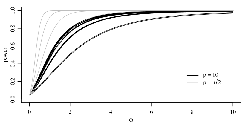
Figure 1: Power of the level-0.05 UMPI test as a function of $\omega$ for various $p$ and $n\in\{20,40,80,160,320\}$.

The power of the level-0.05 test for various values of $p$ and $n$ are shown in Figure 1. Note that the power does not go to one with increasing $n$ if $\omega$ and $p$ are fixed. This makes intuitive sense - in this case the information per row is not increasing while the dimension of ${\mathbf{c}}$ is. However, it should be noted that the power for fixed $n$ and $\omega$ is non-monotonic in $p$: Some numerical calculations (not presented here) indicate that the optimal power for moderate or large values of $n$ or $\omega$ is when $p\approx n/2$, and is somewhat less than this if $n$ and $\omega$ are both small.

It is interesting to note that for this submodel, the likelihood ratio test is quite bad. Straightforward calculations show that the MLE of $\omega$ is $\hat{\omega}=\frac{nt_{{\mathbf{c}}}-p}{p(1-t_{{\mathbf{c}}})}$. Plugging this into the likelihood indicates that a likelihood ratio test is one that rejects when $(n-p)\log(1-t_{{\mathbf{c}}})+p\log t_{{\mathbf{c}}}$ is large. This quantity is not monotonic in the UMPI test statistic $t_{{\mathbf{c}}}$, and performs poorly as a result.

Finally, it is straightforward to extend Theorem 3 to the matrix normal regression model: Consider testing $H:\omega=0$ versus $K:\omega>0$ based on ${\mathbf{Y}}\sim N_{n\times p}({\mathbf{X}}{\mathbf{B}}^{T},\Sigma\otimes(\omega{\mathbf{c}}{\mathbf{c}}^{T}+{\mathbf{I}}))$. As shown in Section 2, any invariant test must depend on ${\mathbf{Y}}$ only through ${\mathbf{G}}(\tilde{{\mathbf{Y}}})=\tilde{{\mathbf{Y}}}(\tilde{{\mathbf{Y}}}^{T}\tilde{{\mathbf{Y}}})^{-1}\tilde{{\mathbf{Y}}}^{T}$, where $\tilde{{\mathbf{Y}}}={\mathbf{H}}{\mathbf{Y}}$. Under the spiked model, $\tilde{{\mathbf{Y}}}\sim N_{(n-q)\times p}({\mathbf{0}},\Sigma\otimes({\mathbf{I}}+\tilde{\omega}\tilde{{\mathbf{c}}}\tilde{{\mathbf{c}}}^{T}))$, where $\tilde{{\mathbf{c}}}={\mathbf{H}}{\mathbf{c}}/||{\mathbf{H}}{\mathbf{c}}||$ and $\tilde{\omega}=\omega||{\mathbf{H}}{\mathbf{c}}||^{2}$. By Theorem 3, the most powerful test of $H$ versus $K$ based on ${\mathbf{G}}(\tilde{{\mathbf{Y}}})$, and hence the most powerful invariant test, is obtained by rejecting when $\tilde{{\mathbf{c}}}^{T}{\mathbf{G}}(\tilde{{\mathbf{Y}}})\tilde{{\mathbf{c}}}$ is large. This quantity can be expressed in more familiar forms as follows:

$$\tilde{{\mathbf{c}}}^{T}{\mathbf{G}}(\tilde{{\mathbf{Y}}})\tilde{{\mathbf{c}}} ={\mathbf{c}}^{T}{\mathbf{H}}^{T}\left[\tilde{{\mathbf{Y}}}(\tilde{{\mathbf{Y}}}^{T}\tilde{{\mathbf{Y}}})^{-1}\tilde{{\mathbf{Y}}}^{T}\right]{\mathbf{H}}{\mathbf{c}}$$

$$={\mathbf{c}}^{T}{\mathbf{H}}^{T}{\mathbf{H}}{\mathbf{Y}}({{\mathbf{Y}}}^{T}{\mathbf{H}}^{T}{\mathbf{H}}{{\mathbf{Y}}})^{-1}{{\mathbf{Y}}}^{T}{\mathbf{H}}^{T}{\mathbf{H}}{\mathbf{c}}$$

$$={\mathbf{c}}^{T}{\mathbf{R}}({\mathbf{R}}^{T}{\mathbf{R}})^{-1}{\mathbf{R}}^{T}{\mathbf{c}}={\mathbf{c}}^{T}{\mathbf{G}}({\mathbf{R}}){\mathbf{c}}.$$

Furthermore, this can also be expressed as ${\mathbf{c}}^{T}({\mathbf{Y}}-{\mathbf{X}}\hat{{\mathbf{B}}}^{T})\hat{\Sigma}^{-1}({\mathbf{Y}}-{\mathbf{X}}\hat{{\mathbf{B}}}^{T})^{T}{\mathbf{c}}/n$, where $\hat{{\mathbf{B}}}^{T}=({\mathbf{X}}^{T}{\mathbf{X}})^{-1}{\mathbf{X}}^{T}{\mathbf{Y}}$ is the OLS estimate of ${\mathbf{B}}^{T}$, and $\hat{\Sigma}={\mathbf{R}}^{T}{\mathbf{R}}/n$ is the MLE of $\Sigma$ under $H$. By Theorem 3, this test statistic has a beta$(p/2,(n-q-p)/2)$ distribution under the null hypothesis.

5 A test of positive row dependence

The UMPI test developed in the previous section is of limited applicability, as typically the space of alternatives of interest is larger than that provided by a spiked covariance model with a fixed eigenvector ${\mathbf{c}}$. However, the UMPI test suggests the possibility of constructing tests based a set of statistics $t_{\mathcal{C}}=\{t_{{\mathbf{c}}}={\mathbf{c}}^{T}{\mathbf{G}}({\mathbf{R}}){\mathbf{c}}:{\mathbf{c}}\in\mathcal{C}\}$, where $\mathcal{C}\subset\mathbb{R}^{n}$ is a set of vectors of particular interest. For example, suppose there is concern that some rows of ${\mathbf{Y}}$ are positively correlated with each other. Based on the results of the previous section, the test statistic $t_{ii^{\prime}}={\mathbf{c}}_{ii^{\prime}}^{T}{\mathbf{G}}({\mathbf{R}}){\mathbf{c}}_{ii^{\prime}}$ could be used to detect positive correlation between rows $i$ and $i^{\prime}$, where ${\mathbf{c}}_{ii^{\prime}}=({\mathbf{e}}_{i}+{\mathbf{e}}_{i^{\prime}})/\sqrt{2}$ is the vector with entries of $1/\sqrt{2}$ in positions $i$ and $i^{\prime}$ and entries of zero elsewhere. However, if there is no information as to which rows might be correlated, some summary of the set of pairwise test statistics $\{t_{{\mathbf{c}}_{ii^{\prime}}}={\mathbf{c}}_{ii^{\prime}}^{T}{\mathbf{G}}({\mathbf{R}}){\mathbf{c}}_{ii^{\prime}}:i\neq i^{\prime}\}$ could be used as a test statistic. Given a residual matrix ${\mathbf{R}}$, the values of these test statistics can be computed quite easily: Some straightforward matrix calculations show that the value of $t_{{\mathbf{c}}_{ii^{\prime}}}$ for $i\neq i^{\prime}$ is given by element $(i,i^{\prime})$ of the matrix ${\mathbf{T}}$, where

$${\mathbf{T}}={\mathbf{G}}({\mathbf{R}})+({\mathbf{g}}{\mathbf{1}}^{T}+{\mathbf{1}}{\mathbf{g}}^{T})/2,$$ (7)

and ${\mathbf{g}}$ is the diagonal of ${\mathbf{G}}({\mathbf{R}})$.

A test for positive dependence among pairs of rows of ${\mathbf{Y}}$ can be based on a scalar summary function of the non-diagonal entries of ${\mathbf{T}}$. Letting $\tilde{t}$ be one such function, the null distribution of $\tilde{t}$ may be obtained via simulation, as the distribution of ${\mathbf{G}}({\mathbf{R}})$ does not depend on any unknown parameters under the null model. A Monte Carlo approximation to the null distribution of $\tilde{t}$ may be obtained via simulation of independent $n\times p$ random matrices ${\mathbf{Y}}^{(1)},\ldots,{\mathbf{Y}}^{(S)}$ with standard normal entries. For each simulated matrix ${\mathbf{Y}}^{(s)}$ a residual matrix ${\mathbf{R}}^{(s)}$ is obtained as determined by the mean model. From ${\mathbf{R}}^{(s)}$, values of ${\mathbf{G}}({\mathbf{R}}^{(s)})$ , ${\mathbf{T}}^{(s)}$ and $\tilde{t}^{(s)}$ may be computed. The critical value for a level-$\alpha$ test based on the test statistic $\tilde{t}$ is approximated by the 1-$\alpha$ quantile of $\tilde{t}^{(1)},\ldots,\tilde{t}^{(S)}$.

The choice of the summary function $\tilde{t}$ may depend on application-specific concerns about a particular type of dependence. Concern about dependence between small number of unspecified rows would suggest using the maximum of the off-diagonal elements of the matrix ${\mathbf{T}}$ in (7) as a test statistic. We refer to this statistic as $t_{\rm max}$, and the resulting test as the maxEP test (maximum exchangeable pair test). Figure 2 shows the power of the level-0.05 maxEP test under the mean-zero model and alternative $\Psi={\mathbf{I}}+\omega{\mathbf{c}}_{ii^{\prime}}{\mathbf{c}}_{ii^{\prime}}^{T}$ for a variety of sample sizes and values of $\omega$ (the choice of $i$ or $i^{\prime}$ does not affect the power). Note that if it were known in advance which pair of rows $(i,i^{\prime})$ were possibly correlated, the UMPI test statistic $t_{{\mathbf{c}}_{ii^{\prime}}}$ could be used, giving the power shown in Figure 1. The difference between Figure 1 and Figure 2 indicates the power loss that results from considering the larger class of alternatives.

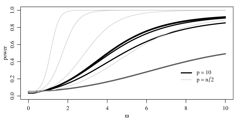
Figure 2: Power of the level-0.05 maxEP test as a function of $\omega$ for various $p$ and $n\in\{20,40,80,160,320\}$.

To illustrate its use, the maxEP test was applied to three datasets using a few different mean models. The first dataset is described in Ashley et al. (2006) and has been analyzed by Efron (2009), among others. The second two datasets are described more fully in Flury (1997). For each test on each dataset, the null distribution was approximated by a Monte Carlo sample of size 5,000. The computer code for implementing these tests is available at my website, http://www.stat.washington.edu/~pdhoff/.

Cardio:

This dataset consists of 20,426 gene expression levels measured on $n=63$ subjects. Although 20,426 gene expression variables are available, any invariant test must be a function of less than 63 of these. Based on the discussion of power that followed Theorem 3, only the first $p=32\approx n/2$ variables were used to perform the test. As in Efron (2009), inference is based on a doubly-centered residual matrix ${\mathbf{R}}$ obtained by de-meaning the rows and columns of the data matrix ${\mathbf{Y}}$, so that ${\mathbf{R}}=({\mathbf{I}}_{n}-{\mathbf{1}}_{n}{\mathbf{1}}_{n}^{T}/n){\mathbf{Y}}({\mathbf{I}}_{p}-{\mathbf{1}}_{p}{\mathbf{1}}_{p}^{T}/p)$. The observed value of $t_{\rm max}$ based on ${\mathbf{R}}$ is .927. In contrast, the largest value of $t_{\rm max}$ observed in the Monte Carlo sample was 0.856, giving an approximate Monte Carlo $p$-value of zero and indicating strong evidence against the null model.

Turtles:

These data consist of length, width and height measurements of 24 male and 24 female turtles, sampled from a single pond on a single day. Two tests were applied to the log-transformed data, the first of which tested $H:\Psi={\mathbf{I}}$ versus $K:\Psi\neq{\mathbf{I}}$ in the column means model, ${\mathbf{Y}}\sim N_{n\times p}({\mathbf{1}}{\boldsymbol{\mu}}^{T},\Sigma\otimes\Psi)$, so that under the null model the rows of ${\mathbf{Y}}$ are i.i.d. $p$-variate normal random vectors. The residual matrix for this mean model is ${\mathbf{R}}=({\mathbf{I}}_{n}-{\mathbf{1}}_{n}{\mathbf{1}}_{n}^{T}/n){\mathbf{Y}}$, which gives an observed $t_{\rm max}$ statistic of 0.344 and a $p$-value of 0.16. The second test is based on the matrix normal regression model (1) where ${\mathbf{X}}$ is the $n\times 2$ matrix indicating the sex of each turtle. The residual matrix here is ${\mathbf{R}}=({\mathbf{I}}-{\mathbf{X}}({\mathbf{X}}^{T}{\mathbf{X}})^{-1}{\mathbf{X}}^{T}){\mathbf{Y}}$, which gives an observed test statistic of $t_{\rm max}=0.336$, corresponding to a $p$-value of 0.20.

Wines:

These data consist of measurements of $p=15$ organic compounds on $n=26$ Riesling wines. Tests were applied to the log-transformed data. The wines were selected from different vintners from three countries, and do not constitute a random sample. Evidence of row covariance was evaluated in the context of the same mean models as for the turtle data - a column means model and a model taking into account a known categorical variable. For the column means model, the $t_{\rm max}$ statistic and the $p$-value for the maxEP test were 0.893 and 0.007 respectively, indicating strong evidence against the null model of i.i.d. measurements. However, after accounting for country differences via the matrix normal regression model (with ${\mathbf{X}}$ being the $n\times 3$ matrix indicating country of origin), the test statistic and $p$-value were 0.843 and 0.23 respectively, indicating little evidence against $H:\Psi={\mathbf{I}}$ after accounting for mean differences due to country.

6 Discussion

The results of this article were developed in the context of a matrix normal error variance model, but they hold more generally for models with stochastic representations of the form ${\mathbf{Y}}={\mathbf{X}}{\mathbf{B}}^{T}+\Psi^{1/2}{\mathbf{Z}}\Sigma^{1/2}$. For example, the characterization of the maximal invariant statistics in Section 2 relies only on the invariance of the model and that ${\mathbf{Z}}$ is full rank with probability one. The results of Sections 3 and 4 depend only on the distribution of the maximal invariant statistic, which in turn depends on ${\mathbf{Z}}$ only through ${\mathbf{W}}={\mathbf{Z}}({\mathbf{Z}}^{T}{\mathbf{Z}})^{-1/2}$. For a normal error variance model the distribution of ${\mathbf{W}}$ is uniform on the Stiefel manifold, but this is also true for any model where the distribution of the vectorization of ${\mathbf{Z}}$ is spherically symmetric. The class of models for ${\mathbf{Y}}$ in which $\text{vec}({\mathbf{Z}})$ is spherically symmetric are the elliptically contoured matrix distributions (Gupta and Varga, 1994), which includes heavy-tailed and contaminated distributions, among others.

This article has considered tests of $H:\Psi={\mathbf{I}}$ versus $K:\Psi\neq{\mathbf{I}}$, that is, tests of whether or not the rows of the error matrix ${\mathbf{Y}}-{\mathbf{X}}{\mathbf{B}}^{T}$ are independent and identically distributed. This null hypothesis is violated not just when the rows are dependent, but also when they are heteroscedastic and independent. However, in some applications it may be useful to have a test that includes independent heteroscedasticity as part of the null hypothesis. Volfovsky and Hoff (2015) studied a likelihood ratio test of $H:(\Sigma,\Psi)\in\mathcal{D}_{p}^{+}\times\mathcal{D}_{n}^{+}$ versus $K:(\Sigma,\Psi)\notin\mathcal{D}_{p}^{+}\times\mathcal{D}_{n}^{+}$, where $\mathcal{D}_{k}^{+}$ is the set of $k\times k$ diagonal matrices with positive entries. However, their test is only applicable to square data matrices, and will reject in the presence of either row or column dependence. For testing $H:\Psi\in\mathcal{D}_{n}^{+}$ versus $K:\Psi\not\in\mathcal{D}_{n}^{+}$ it might be possible to use invariance, but perhaps not directly: A natural group with which to find an invariant procedure are the transformations of the form $g({\mathbf{Y}})={\mathbf{A}}{\mathbf{Y}}{\mathbf{B}}^{T}$, where ${\mathbf{A}}\in\mathcal{D}_{n}^{+}$ and ${\mathbf{B}}\in\mathbb{R}^{p\times p}$ is nonsingular. However, while the covariance model is invariant to such transformations the mean model is not, and so it seems that to usefully apply invariance one would first need to reduce to a mean-zero model, as was done in Section 2.3 for mean models with row effects.

References

- Ashley et al. (2006) Ashley, E. A., R. Ferrara, J. Y. King, A. Vailaya, A. Kuchinsky, X. He, B. Byers, U. Gerckens, S. Oblin, A. Tsalenko, et al. (2006). Network analysis of human in-stent restenosis. Circulation 114(24), 2644–2654.
- Chikuse (2003) Chikuse, Y. (2003). Statistics on special manifolds, Volume 174 of Lecture Notes in Statistics. New York: Springer-Verlag.
- Dawid (1981) Dawid, A. P. (1981). Some matrix-variate distribution theory: notational considerations and a Bayesian application. Biometrika 68(1), 265–274.
- Efron (2009) Efron, B. (2009). Are a set of microarrays independent of each other? Ann. Appl. Stat. 3(3), 922–942.
- Flury (1997) Flury, B. (1997). A first course in multivariate statistics. Springer Texts in Statistics. Springer-Verlag, New York.
- Gupta and Varga (1994) Gupta, A. and T. Varga (1994). A new class of matrix variate elliptically contoured distributions. Journal of the Italian Statistical Society 3(2), 255–270.
- Gupta and Nagar (2000) Gupta, A. K. and D. K. Nagar (2000). Matrix variate distributions, Volume 104 of Chapman & Hall/CRC Monographs and Surveys in Pure and Applied Mathematics. Boca Raton, FL: Chapman & Hall/CRC.
- Mardia et al. (1979) Mardia, K. V., J. T. Kent, and J. M. Bibby (1979). Multivariate analysis. London: Academic Press [Harcourt Brace Jovanovich Publishers]. Probability and Mathematical Statistics: A Series of Monographs and Textbooks.
- Muralidharan (2010) Muralidharan, O. (2010). Detecting column dependence when rows are correlated and estimating the strength of the row correlation. Electron. J. Stat. 4, 1527–1546.
- Volfovsky and Hoff (2015) Volfovsky, A. and P. D. Hoff (2015). Testing for Nodal Dependence in Relational Data Matrices. J. Amer. Statist. Assoc. 110(511), 1037–1046.