This is the peer reviewed version of the following article: STAT, 5, (2016), 286-294, which has been published in final form at doi:10.1002/sta4.122. This article may be used for non-commercial purposes in accordance with Wiley Terms and Conditions for Self-Archiving; also on Arxiv 1512.09016.

Pairwise Markov properties for regression graphs

Kayvan Sadeghi
University of Cambridge, Cambridge, UK

Nanny Wermuth

Chalmers University of Technology, Gothenburg, Sweden and Gutenberg-University, Mainz, Germany

Abstract: With a sequence of regressions, one may generate joint probability distributions. One starts with a joint, marginal distribution of context variables having possibly a concentration graph structure and continues with an ordered sequence of conditional distributions, named regressions in joint responses. The involved random variables may be discrete, continuous or of both types. Such a generating process specifies for each response a conditioning set which contains just its regressor variables and it leads to at least one valid ordering of all nodes in the corresponding regression graph which has three types of edge; one for undirected dependences among context variables, another for undirected dependences among joint responses and one for any directed dependence of a response on a regressor variable. For this regression graph, there are several definitions of pairwise Markov properties, where each interprets the conditional independence associated with a missing edge in the graph in a different way. We explain how these properties arise, prove their equivalence for compositional graphoids and point at the equivalence of each one of them to the global Markov property.
Keywords: Chain graph; compositional graphoid; graphical Markov model; intersection; pairwise Markov property; sequence of regressions.

1 Introduction

Regression graph models are the subclass of graphical Markov models that is best suited to capture pathways of development, no matter whether the generating process arises in observational studies or in intervention studies, see Wermuth (2015). For prospective studies, time provides a partial ordering of a finite number of variables and leads to an ordered sequence of joint and single response variables. In other studies, any ordering is provisional but, typically, may be agreed upon by researchers in the given field of study.

Regression graph models extend models proposed by Cox & Wermuth (1993), illustrated there with several small sets of data having some joint responses and just linear relations; for linear regressions see e.g. Weisberg (2014). Additional in regression graph models are context variables which capture baseline features of study individuals or of study conditions. Context variables may be controlled or fixed by study design. Regression graphs represent an essential extension of fully directed acyclic graphs whenever one wants to model that explanatory variables affect directly several response variables at the same time and to take the baseline information of context variables explicitly into account.

Individual random variables can be continuous, discrete or of both types. For such mixed responses, the conditional distributions may, for instance, be conditional Gaussian regressions; see Lauritzen & Wermuth (1989), be approximated by generalized linear regressions; see McCullagh & Nelder (1989), Andersen & Skovgaard (2010), or if needed, be any other type of nonlinear regression, which permits to represent the relevant conditional independences and dependences.

For discrete variables, ordered sequences of joint regressions without context variables have been studied as chain graph models of type IV by Drton (2009). A parameterization and maximum-likelihood estimates were derived by Marchetti & Lupparelli (2011).

For context variables in general, the independence structure is captured by an undirected graph in vertex set $V=\{1,\ldots,d_{V}\}$ and edge set $E$, known as the concentration graph. The name reminds one that for regular joint Gaussian distributions, a missing edge for vertex pair $i,j$ shows as an $ij$-zero in its concentration matrix, the inverse covariance matrix; see Dempster (1972), Cox & Wermuth (1993). In general, at most one undirected $ij$-edge, $i\mbox{$\,\frac{\hskip 4.89998pt\hskip 4.89998pt\;}{\hskip 4.89998pt\hskip 4.89998pt}$}j$, couples the vertices $i,j$, and each missing edge for $i,j$ means $X_{i}$ is independent of $X_{j}$ given the remaining variables. This is written compactly in terms of vertices, also called nodes, as $i\mbox{{ $\perp\perp$ }}j|V\setminus\{i,j\}$; see Dawid (1979).

For exclusively discrete context variables, the joint distributions have been studied as Markov fields and log-linear interaction models; see Darroch, Lauritzen & Speed (1980), named later also discrete concentration graph models. For these, one also knows when single unobserved variables can be identified; see Stanghellini & Vantaggi (2013).

For regression graphs in node set $N=\{1,\ldots d\},$ where each node represents a variable, the edge set contains in general three types of edge of different interpretation. The $ij$-edge among two context nodes is denoted by a full line, $i\mbox{$\,\frac{\hskip 4.89998pt\hskip 4.89998pt\;}{\hskip 4.89998pt\hskip 4.89998pt}$}j$. Edges for directed dependences are $ij$-arrows, $i\mbox{$\hskip 0.50003pt\prec\!\!\!\!\!\frac{\hskip 4.89998pt\hskip 4.89998pt}{\hskip 4.89998pt}$}j$. Each $ij$-arrow starts at a regressor node $j$ and points to a response $i$. The $ij$-edge between two individual response nodes within a given joint response is denoted by a dashed line, $i\mbox{$\frac{\hskip 2.45004pt}{\hskip 2.45004pt}\frac{\;\,}{\;}\frac{\hskip 2.45004pt}{\hskip 2.45004pt}$}j$. In some literature, this is replaced by an double-headed arrow. Undirected graphs of this type are named conditional covariance graphs to remind one that for joint Gaussian distributions, a missing $ij$-edge shows as an $ij$-zero in the conditional covariance matrix of a joint response $X\!:=(X_{1},\ldots X_{p})$, given the union of their individual regressors.

Among the results available so far for regression graphs are (1) a simple graphical criterion to decide whether two regression graphs, with the same node and edge set but different types of edge, define the same independence structure; see Wermuth & Sadeghi (2012), (2) path criteria and zero-matrix criteria for separation; see Sadeghi & Lauritzen (2014), Wermuth (2015), (3) induced graphs, after marginalising over some nodes and conditioning on others, which preserve the independence structure of the generating regression graph, see Sadeghi (2013), (4) induced graphs, which only predict dependences generated by a regression graph between $X_{\alpha}$ and $X_{\beta}$ given $X_{c}$, for disjoint $\alpha,\beta,c,m$ partitioning $N$. This requires an edge-minimal graph, that is one in which no edge can be removed without introducing another independence constraint; see Wermuth (2012), (5) implementations in the computing environment R; see Sadeghi & Marchetti (2012).

Independence properties implied by the standard graph theoretic separation criterion on graphs listed here as $(i)$ to $(v)$ in Section 3, were introduced by Pearl & Paz (1987) for concentration graphs and said to define a graphoid. More importantly, they derived that for graphoids all independences implied by the given graph, may be obtained either from the list of independences defined by its missing edges or by separation in undirected graphs. This became known later as the equivalence of the pairwise Markov property and the global Markov property.

Such an equivalence has been proven for more general classes of graphs, including regression graphs, for which the global Markov property is also generalized compared to concentration graphs; see Sadeghi & Lauritzen (2014). This uses the additional independence property of composition, listed here as property $(vi)$ in Section 4. For such compositional graphoids, several pairwise Markov properties may be defined, which give alternative independence interpretations to a missing edge. One question to be solved was whether each of them is suitable to derive the regression-graph structure that is all independences implied by the graph.

Here, we define four pairwise Markov properties and show with Theorem 1 that they are equivalent with respect to regression graphs. Thus, any one of the four pairwise properties characterizes the regression-graph structure. By using the equivalence of one of them to the global Markov property, proven in Sadeghi & Lauritzen (2014), it follows that each one is also equivalent to the global Markov property.

The smallest conditioning set for the independence of two response components will be shown to be the set of important regressors for just one of the responses. This result for independences is of special importance since it contrasts with a well-known result for estimating the dependences of responses on their regressors: when strong residual dependences remain among the responses, after one has been regressing each response component separately on different sets of regressors, distorted parameter estimates may be obtained, see Haavelmo (1943), Zellner (1962), Drton & Richardson (2004). For an exposition of these ideas in terms of Gaussian variables, standardized to have zero means and unit variances, see Cox & Wermuth (1993), beginning of Section 4.

We introduce in Section 2 more definitions and concepts for regression graphs. In Section 3, we provide independence properties, give four pairwise Markov properties for regression graphs, and prove their equivalence for compositional graphoids. We end with a discussion in Section 4.

2 Some more definitions and concepts for regression graphs

A simple graph with a finite node set $N=\{1,\dots,d\}$ has in its edge set $E$ at most one $ij$-edge for nodes $i,j$ in $N$. When $i,j$ are the endpoints of an edge, the node pair is said to be coupled or to be adjacent and denoted by $i\sim j$. A simple graph is complete when all pairs are coupled by an edge.

A parent of node $i$ is the starting node $j$ of an arrow pointing to $i$ and indicates a regressor variable $X_{j}$ of response $X_{i}$. The set of parents of a node $i$ is denoted by $\mathrm{par}(i)$. An $ij$-path is a sequence of edges passing through distinct inner nodes, connecting the endpoints $i$ and $j$ of the path. By convention, an $ij$-edge is the shortest type of path.

A subgraph induced by a subset $a$ of $N$ consists of the node set $a$ and of the edges present in the graph among the nodes of $a$. A subgraph is connected if there is a path between any distinct node pair. A maximally connected subgraph is called a connected component.

A direction-preserving $ij$-path to $i$ from $j$ consists of arrows, all pointing from $j$ towards $i$. In such a direction-preserving path, node $j$ is named an ancestor of $i$. An anterior $ij$-path consists of a direction-preserving path followed by an undirected path, such as:

$$i\ \mbox{$\hskip 0.50003pt\prec\!\!\!\!\!\frac{\hskip 4.89998pt\hskip 4.89998pt}{\hskip 4.89998pt}$}\underbrace{\overbrace{\mbox{\large{$\mbox{$\circ$}$}}\mbox{$\hskip 0.50003pt\prec\!\!\!\!\!\frac{\hskip 4.89998pt\hskip 4.89998pt}{\hskip 4.89998pt}$}\mbox{\large{$\mbox{$\circ$}$}},\ldots,\mbox{\large{$\mbox{$\circ$}$}}\mbox{$\hskip 0.50003pt\prec\!\!\!\!\!\frac{\hskip 4.89998pt\hskip 4.89998pt}{\hskip 4.89998pt}$}\mbox{\large{$\mbox{$\circ$}$}}}^{\text{\normalsize{ancestors of {i}}}}\mbox{$\,\frac{\hskip 4.89998pt\hskip 4.89998pt\;}{\hskip 4.89998pt\hskip 4.89998pt}$}\mbox{\large{$\mbox{$\circ$}$}}\mbox{$\,\frac{\hskip 4.89998pt\hskip 4.89998pt\;}{\hskip 4.89998pt\hskip 4.89998pt}$}\mbox{\large{$\mbox{$\circ$}$}},\ldots,\mbox{\large{$\mbox{$\circ$}$}}\mbox{$\,\frac{\hskip 4.89998pt\hskip 4.89998pt\;}{\hskip 4.89998pt\hskip 4.89998pt}$}j}_{\text{\normalsize{anteriors of {i}}}}.$$

Thus, anterior nodes extend the notion of ancestors. The set of anterior nodes of node $i$ is denoted by $\mathrm{ant}(i)$.

The regression graph, $G^{N}_{\mathrm{reg}}\,$​, is a simple graph with a finite node set $N$​ and an edge set of three different types of edge. Here we use arrows, dashed and full lines. The properties of $G^{N}_{\mathrm{reg}}\,$are (1) no arrow points to a full line and no dashed line is adjacent to a full line, (2) there is a valid ordering of its unique set of connected components, $(g_{1},\dots,g_{Q})$. These components result by removing all arrows from $G^{N}_{\mathrm{reg}}\,$​. The connected components of dashed lines can be ordered such that $g_{q}<g_{l}$ if there is an arrow pointing to a node in $g_{q}$ from a node in $g_{l}$. Connected components of full lines have a higher order than those of dashed lines and can be ordered in any way.

The induced subgraph of $G^{N}_{\mathrm{reg}}\,$of only arrows and dashed lines is called the response set, $u$, the complimentary one of only full lines is the context set, $v$ so that $N=(u,v).$ Accordingly, connected components of $u$ are the response components, those of $v$ are the context components. For a node $i$ in response set $g_{q}$, its past is denoted by $\mathrm{pst}(i)$ and it consists of all nodes in components having a higher order than $g_{q}$.

Although for the regression-graph structure, only a valid ordering of its connected components is essential, one can indeed extend a valid ordering of these components into a complete valid ordering of all nodes, $(1,\dots,N)$, where $i<j$ if $q<l$ for $i\in g_{q}$ and $j\in g_{l}$. This implies that $i<j$ if there is an arrow pointing to $i$ from $j$. The past of a node $i$ in response component $g_{q}$ contains never any node $j$ of $g_{q}$ even if $j$ is larger in a complete valid ordering of the nodes.

Conditional independences are captured by missing edges in $G^{N}_{\mathrm{reg}}\,$​. A missing edge for $i,j$ in $G^{N}_{\mathrm{reg}}\,$is denoted by $i\nsim j$. For $i\nsim j$, there is some subset $c$ of $N\setminus\{i,j\}$ such that in the graph $X_{i}$ is conditionally independent of $X_{j}$ given $X_{c}$, written as $i\mbox{{ $\perp\perp$ }}j|c$. Four different ways of defining $c$ are studied in the next Section 3.

3 Pairwise Markov properties for regression graphs

The following properties have been defined for conditional independences of probability distributions. Let $a,b,d,c$ be disjoint subsets of $N$, where $c$ may be the empty set.

• $(i)$ symmetry: $a\mbox{{ $\perp\perp$ }}b|c{\implies}b\mbox{{ $\perp\perp$ }}a|c$ ;

• $(ii)$ decomposition: $a\mbox{{ $\perp\perp$ }}bd|c{\implies}(a\mbox{{ $\perp\perp$ }}b|c$ and $a\mbox{{ $\perp\perp$ }}d|c$) ;

• $(iii)$ weak union: $a\mbox{{ $\perp\perp$ }}bd|c{\implies}(a\mbox{{ $\perp\perp$ }}b|dc$ and $a\mbox{{ $\perp\perp$ }}d|bc$) ;

• $(iv)$ contraction: $(a\mbox{{ $\perp\perp$ }}b|dc$ and $a\mbox{{ $\perp\perp$ }}d|c)\iff a\mbox{{ $\perp\perp$ }}bd|c$ ;

• $(v)$ intersection: ( $a\mbox{{ $\perp\perp$ }}d|bc$ and $a\mbox{{ $\perp\perp$ }}b|dc){\implies}a\mbox{{ $\perp\perp$ }}bd|c$ ;

• $(vi)$ composition: ($a\mbox{{ $\perp\perp$ }}d|c$ and $a\mbox{{ $\perp\perp$ }}b|c){\implies}a\mbox{{ $\perp\perp$ }}bd|c$ .

Note that composition defines the reverse direction of decomposition. Intersection gives the reverse direction of weak union and properties $(i)$ to $(iv)$ are the independence properties of all probability distributions; see Dawid (1979), Studený (1989).

The first five independence properties, listed above, give the graphoids of Pearl & Paz (1987), see also Studený (1989, 2005). If, in addition, the composition property holds, one speaks of a compositional graphoid. For compositional graphoids, pairwise independences can be combined to obtain global independence statements of the type $a\mbox{{ $\perp\perp$ }}b|c$ for general classes of graphs, which include regression graphs; see Sadeghi & Lauritzen (2014). Thus, the above six properties are also satisfied by $G^{N}_{\mathrm{reg}}\,$​. They are the properties used here in the proof of Theorem 1.

Let $G^{N}_{\mathrm{reg}}\,$be a regression graph with a valid ordering of the node set $N=(1,\dots,d)$, which necessarily conforms with a valid ordering of its connected components. Based on this ordering, we always assume in this section that $i<j$ for the node pair $i,j$. To define pairwise Markov properties for $G^{N}_{\mathrm{reg}}\,$​, we use the following notation for parents, anteriors and the past of node pair $i,j$:

$$\mathrm{par}(i,j) = \mathrm{par}(i)\cup\mathrm{par}(j)\setminus\{i,j\},$$

$$\mathrm{ant}(i,j) = \mathrm{ant}(i)\cup\mathrm{ant}(j)\setminus\{i,j\},$$

$$\mathrm{pst}(i,j) = \mathrm{pst}(i)\cup\mathrm{pst}(j)\setminus\{i,j\}.$$

The distribution $\mathcal{P}$ of $(X_{n})_{n\in N}$ satisfies a pairwise Markov property $(Pm)$, for $m=1,2,3,4$, with respect to $G^{N}_{\mathrm{reg}}\,$if for $i$ and $j$ in the context set, $v$,

$$i\not\sim j \implies i\mbox{{ $\perp\perp$ }}j|v\setminus\{i,j\}\,,$$

and for $i$ in the response set, $u$,

$$(P1):i\not\sim j \implies i\mbox{{ $\perp\perp$ }}j|\mathrm{pst}(i,j)\,,$$

$$(P2):i\not\sim j \implies i\mbox{{ $\perp\perp$ }}j|\mathrm{ant}(i,j)\,,$$

$$(P3):i\not\sim j \implies i\mbox{{ $\perp\perp$ }}j|\mathrm{par}(i,j)\,,$$

$$(P4):i\not\sim j \implies i\mbox{{ $\perp\perp$ }}j|\mathrm{par}(i).$$

Notice that in (P4), $\mathrm{par}(i)$ may be replaced by $\mathrm{par}(j)$ whenever the two nodes are in the same connected component. Consider, for example, the graph of Figure 1 with $N=(1,\ldots,9)$.

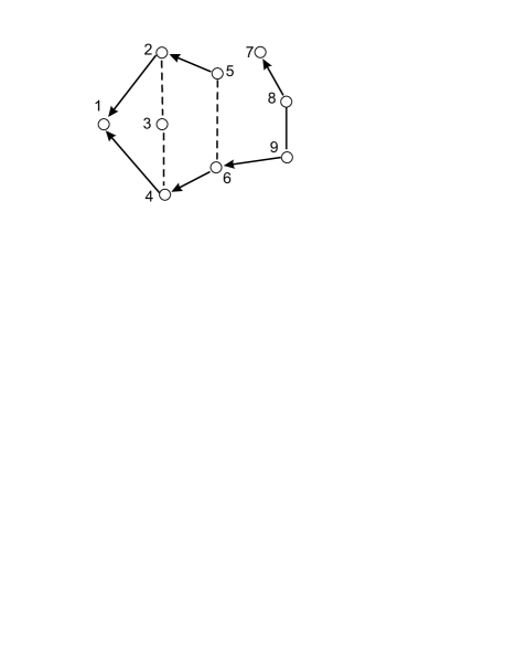
Figure 1: A regression graph.

For the uncoupled pair of nodes $2,4$, the nodes in its past are $\mathrm{pst}(2,4)=\{5,6,7,8,9\}$, the anteriors are $\mathrm{ant}(2,4)=\{5,6,8,9\}$, the parents are $\mathrm{par}(2,4)=\{5,6\}$ while the parent of node $2$ alone is node $5$, so that by the four pairwise Markov properties, listed here including their conditioning sets,

$$(P1),\text{past} \implies 2\mbox{{ $\perp\perp$ }}4|\{5,6,7,8,9\};$$

$$(P2),\text{anteriors} \implies 2\mbox{{ $\perp\perp$ }}4|\{5,6,8,9\};$$

$$(P3),\text{joint parents} \implies 2\mbox{{ $\perp\perp$ }}4|\{5,6\};$$

$$(P4),\text{parents of the smaller node} \implies 2\mbox{{ $\perp\perp$ }}4|5.$$

Theorem 1.

Let a distribution $\mathcal{P}$ of $(X_{n})_{n\in N}$ be a compositional graphoid. Then, for every valid ordering of the nodes of $G^{N}_{\mathrm{reg}}\,$​, $\mathcal{P}$ satisfies $(P1)\iff(P2)\iff(P3)\iff(P4)$ with respect to $G^{N}_{\mathrm{reg}}\,$​.

Before presenting the proof, we provide the following example related to the graph of Figure 1, in which we follow the same method as in the proof of this theorem that is using compositional graphoid properties to obtain the equivalence of the independence statements implied by the different pairwise Markov properties:

$(P1)\Rightarrow(P2):$ By definition, we have $2\mbox{{ $\perp\perp$ }}4|\{5,6,7,8,9\}$ and $4\mbox{{ $\perp\perp$ }}7|\{5,6,8,9\}$. Contraction implies $4\mbox{{ $\perp\perp$ }}\{2,7\}|\{5,6,8,9\}$. Then, decomposition gives that $2\mbox{{ $\perp\perp$ }}4|\{5,6,8,9\}$.

$(P2)\Rightarrow(P3):$ Nodes $6,8$ and $9$ are in the set $\mathrm{ant}(2,4)\setminus\mathrm{par}(2)$, and it holds that $2\mbox{{ $\perp\perp$ }}8|\{5,6,9\}$, $2\mbox{{ $\perp\perp$ }}9|\{5,6,8\}$, and $2\mbox{{ $\perp\perp$ }}6|\{5,8,9\}$. Intersection, used repeatedly, implies $2\mbox{{ $\perp\perp$ }}\{6,8,9\}|5$. This together with $2\mbox{{ $\perp\perp$ }}4|\{5,6,8,9\}$ implies by contraction $2\mbox{{ $\perp\perp$ }}\{4,6,8,9\}|5$. By decomposition, $2\mbox{{ $\perp\perp$ }}\{4,6\}|5$ so that by weak union, $2\mbox{{ $\perp\perp$ }}4|\{5,6\}$.

$(P3)\Rightarrow(P4):$ By contraction, $2\mbox{{ $\perp\perp$ }}9|5$ and $2\mbox{{ $\perp\perp$ }}6|\{9,5\}$, imply $2\mbox{{ $\perp\perp$ }}\{6,9\}|5$, which by decomposition implies $2\mbox{{ $\perp\perp$ }}6|5$. By contraction, this and $2\mbox{{ $\perp\perp$ }}4|\{5,6\}$ imply $2\mbox{{ $\perp\perp$ }}\{4,6\}|5$ so that by decomposition $2\mbox{{ $\perp\perp$ }}4|5$.

$(P4)\Rightarrow(P1):$ Composition used repeatedly for statements $2\mbox{{ $\perp\perp$ }}4|5$, $2\mbox{{ $\perp\perp$ }}6|5$, $2\mbox{{ $\perp\perp$ }}7|5$, $2\mbox{{ $\perp\perp$ }}8|5$, $2\mbox{{ $\perp\perp$ }}9|5$ gives $2\mbox{{ $\perp\perp$ }}\{4,6,7,8,9\}|5$. Weak union implies $2\mbox{{ $\perp\perp$ }}4|\{5,6,7,8,9\}$.

Proof of Theorem 1.

$(P1)\Rightarrow(P2):$ By definition, $\mathrm{pst}(i,j)=\mathrm{pst}(i)\setminus\{j\}$. Let $k\in\{j\}\cup\mathrm{pst}(i)\setminus\mathrm{ant}(i,j)$, then $k\nsim i$ and $i\mbox{{ $\perp\perp$ }}k|\mathrm{pst}(i)\setminus\{k\}$. For another possible node $l\in\mathrm{pst}(i)\setminus\mathrm{ant}(i,j)$ holds also that $i\mbox{{ $\perp\perp$ }}l|\mathrm{pst}(i)\setminus\{l\}$. By the intersection property, we obtain $i\mbox{{ $\perp\perp$ }}\{k,l\}|\mathrm{pst}(i)\setminus\{k,l\}$. By the same method and an inductive argument, for all members of $\mathrm{pst}(i)\setminus\mathrm{ant}(i,j)$, we obtain $i\mbox{{ $\perp\perp$ }}\mathrm{pst}(i)\setminus\mathrm{ant}(i,j)|\mathrm{ant}(i,j)$. Now if $i$ and $j$ are in different connected components then by the same method, we use the intersection property to obtain $i\mbox{{ $\perp\perp$ }}\{j\}\cup\mathrm{pst}(i)\setminus\mathrm{ant}(i,j)|\mathrm{ant}(i,j)$, and if $i$ and $j$ are in the same connected component, we use the contraction property with $i\mbox{{ $\perp\perp$ }}j|\mathrm{pst}(i)$ to obtain the same independence statement. The decomposition property yields $i\mbox{{ $\perp\perp$ }}j|\mathrm{ant}(i,j)$.

$(P2)\Rightarrow(P3):$ Suppose that $i$ is in the lower or equal index component $g_{r}$ than that of $j$. Let also $k\in\mathrm{ant}(i,j)\setminus\mathrm{par}(i)$. Notice that $k\nsim i$ since $k\not\in\mathrm{par}(i)$ and if, $k\in\mathrm{ant}(j)\setminus\mathrm{ant}(i)$ and adjacent to $i$ then $i$ is of a higher order than $j$, which is not possible. We prove that $i\mbox{{ $\perp\perp$ }}k|\mathrm{ant}(i)\setminus\{k\}$:

If $k\in\mathrm{ant}(i)$ then $\mathrm{ant}(k)\subset\mathrm{ant}(i)$ and subsequently $\mathrm{ant}(i,k)=\mathrm{ant}(i)$. The result is then obvious from the assumption. Thus assume that $k\in\mathrm{ant}(j)\setminus\mathrm{ant}(i)$. We then use reverse induction on the order of the connected components in which $k$ lies to prove the claim. For the base, we have that $k$ is in $g_{v}$, and let $g_{v,k}$ be the connected component containing $k$ in $g_{v}$. It holds that $\mathrm{ant}(k)=g_{v,k}$. For every member $l$ of $g_{v,k}$, it holds that $i\mbox{{ $\perp\perp$ }}l|\mathrm{ant}(i)\cup g_{v,k}$. By intersection, for all such statements, we obtain $i\mbox{{ $\perp\perp$ }}g_{v,k}|\mathrm{ant}(i)$. Decomposition implies the result.

Now suppose that $k\in g_{q}$ and, for every $l\in\mathrm{ant}(k)\setminus\mathrm{ant}(i)$, by the induction hypothesis, it holds that $i\mbox{{ $\perp\perp$ }}l|\mathrm{ant}(i)$. By the composition property for all such $i\mbox{{ $\perp\perp$ }}l|\mathrm{ant}(i)$, we obtain that $i\mbox{{ $\perp\perp$ }}\mathrm{ant}(k)\setminus\mathrm{ant}(i)|\mathrm{ant}(i)$. This together with $i\mbox{{ $\perp\perp$ }}k|\mathrm{ant}(i,k)$, by using the contraction property, implies that $i\mbox{{ $\perp\perp$ }}\{k\}\cup\mathrm{ant}(k)\setminus\mathrm{ant}(i)|\mathrm{ant}(i)\setminus\{k\}$. The decomposition property gives $i\mbox{{ $\perp\perp$ }}k|\mathrm{ant}(i)\setminus\{k\}$.

Now by the intersection property for all such $i\mbox{{ $\perp\perp$ }}k|\mathrm{ant}(i)\setminus\{k\}$, we obtain $i\mbox{{ $\perp\perp$ }}\mathrm{ant}(i,j)\setminus\mathrm{par}(i)|\mathrm{par}(i)$. This together with $i\mbox{{ $\perp\perp$ }}j|\mathrm{ant}(i,j)$, using the contraction property, implies $i\mbox{{ $\perp\perp$ }}\{j\}\cup\mathrm{ant}(i,j)\setminus\mathrm{par}(i)|\mathrm{par}(i)$. By the decomposition property, this gives $i\mbox{{ $\perp\perp$ }}\{j\}\cup\mathrm{par}(j)\setminus\mathrm{par}(i)|\mathrm{par}(i)$. The weak union property now implies $i\mbox{{ $\perp\perp$ }}j|\mathrm{par}(i,j)$.

$(P3)\Rightarrow(P4):$ We prove the result by reverse induction on the order of the connected component that contains $j$. If $j$ is in $g_{v}$ then the result trivially holds. Thus suppose that $j$ lies in $g_{q}$. By induction hypothesis for each $k\in\mathrm{par}(j)\setminus\mathrm{par}(i)$ we have $i\mbox{{ $\perp\perp$ }}k|\mathrm{par}(i)$. By the composition property, it is implied that $i\mbox{{ $\perp\perp$ }}\mathrm{par}(j)\setminus\mathrm{par}(i)|\mathrm{par}(i)$. This together with $i\mbox{{ $\perp\perp$ }}j|\mathrm{par}(i,j)$, by the contraction property, implies $i\mbox{{ $\perp\perp$ }}\{j\}\cup\mathrm{par}(j)\setminus\mathrm{par}(i)|\mathrm{par}(i)$. The decomposition property now gives $i\mbox{{ $\perp\perp$ }}j|\mathrm{par}(i)$.

$(P4)\Rightarrow(P1):$ Suppose that $k\in\{j\}\cup\mathrm{pst}(i,j)\setminus\mathrm{par}(i)$. We have that $k\nsim i$. Therefore, $i\mbox{{ $\perp\perp$ }}k|\mathrm{par}(i)$. Using the composition property for all such statements for members of $\{j\}\cup\mathrm{pst}(i,j)\setminus\mathrm{par}(i)$, we obtain $i\mbox{{ $\perp\perp$ }}\{j\}\cup\mathrm{pst}(i,j)\setminus\mathrm{par}(i)|\mathrm{par}(i)$. The weak union property implies $i\mbox{{ $\perp\perp$ }}j|\mathrm{pst}(i.j)$. ∎

Based on the equivalence of the global Markov property and the pairwise Markov property $(P2)$, proven in Sadeghi & Lauritzen (2014), we have the following corollary:

Corollary 1.

Let a distribution $\mathcal{P}$ of $(X_{n})_{n\in N}$ be a compositional graphoid. Then, for every valid ordering of the nodes of $G^{N}_{\mathrm{reg}}\,$, $\mathcal{P}$ satisfies the global Markov property with respect to $G^{N}_{\mathrm{reg}}\,$if and only if it satisfies any one of $(P1)$, $(P2)$, $(P3)$, or $(P4)$.

It is a consequence of the above results that in case one of the four pairwise independence properties is satisfied, all other three hold as well so that, depending on the purpose of an enquiry, each one of them may be used. The results have been applied implicitly in model-fitting strategies which also include checks of necessary conditions for properties $(v)$ to $(vii)$; see e.g. Wermuth & Sadeghi (2012), Appendix; Wermuth & Cox (2013), Appendix.

There is an additional independence property, needed for studying dependences induced by a given edge-minimal graph,

• $(vii)$ singleton transitivity: ($j\mbox{{ $\perp\perp$ }}k|c$ and $j\mbox{{ $\perp\perp$ }}k|ic){\implies}(i\mbox{{ $\perp\perp$ }}j|c$ or $i\mbox{{ $\perp\perp$ }}k|c$),

where $i,j,k$ are distinct nodes of node set $N$ and $c\subseteq N\setminus\{i,j,k\}$. Probability distributions satisfying this property of singleton transitivity in addition to $(i)$ to $(vi)$ are for instance regular joint Gaussian distributions; see Lněnička & Matúš (2007), and totally positive distributions with positive support everywhere; see Fallat et al (2016).

The above seven properties of a density generated over $G^{N}_{\mathrm{reg}}\,$ensure that the graph may be used to trace pathways of dependences, see Wermuth (2012, 2015). Such a sequence of regressions has therefore been said to be traceable.

4 Discussion

For regression graphs and for distributions that are compositional graphoids, the equivalence of four different pairwise independence properties has been proven, two of which, $(P1)$ and $(P4)$, require a valid ordering of all variables. Together with the known equivalence of one of them, $(P2)$, to the global Markov property, this gives essential insights into regression-graph structures and, at the same time, into the structural independence constraints of such distributions that is into independences which hold irrespective of specific parameter values for a given regression graph model.

For the same set of context variables, different special parametrizations for the directed dependences of main interest may arise, for instance, just with differing baseline conditions that is with different realisations for the context variables. Hence, especially for comparing results from several studies with the same variables, it is essential to be able to distinguish between structural independences and those which result only with specific constellations of parameters. The former are captured by a generating regression graph and the latter by parameter estimates given a set of data.

The conditioning set is largest for the past of any two non-adjacent nodes, $(P1)$, and smallest for the subset of this past containing just the parents of one of the two nodes, $(P4)$. The two other properties have conditioning sets of intermediate size, they may be larger than those for $(P4)$ but they are never larger than those for $(P1)$. This implies for a regression graph what follows for the generated distribution by its factorization in terms of connected components: variables outside the past of a missing edge need not be considered for its independence interpretation.

For any given joint response, property $(P4)$ justifies the elimination of unimportant regressors for each response component separately, but only with property $(P3)$, that is by conditioning on the joint parents of two response nodes, possible estimation problems are avoided, such as in seemingly unrelated regressions. By using $(P3)$, a reduced model is replaced by a covering model which is simpler concerning estimation properties; see Cox & Wermuth (1990). In the Gaussian case for a reduced model of seemingly unrelated regressions, the covering model is the so-called general linear model which has identical sets of regressors for each response pair; see Anderson (1958).

For tracing pathways of dependence, the pairwise property given the anterior set of a node, $(P2)$ is the essential one. Intervening early at an inner node of an anterior path in an edge-minimal graph will interrupt a pathway of development. For instance with exclusively strong risk factors along such a path, an early intervention may stop an otherwise disastrous accumulation of risks.

The main importance of the pairwise property given the past of a node pair, $(P1)$, is that independence constraints and pairwise dependences are defined without any change in this largest conditioning set. This permits to extend a given connected graph into a complete graph by keeping its given valid node ordering: all missing full lines in the context set are added, in each response component dashed lines are added until its subgraph is complete, then for each remaining node pair with $i<j$, an arrow pointing to $i$ from $j$ is added. This helps to understand which constraints have been imposed on this completed graph to obtain the given missing edges.

The completed graph leads also to the factorization of a generated distribution in terms of connected components but without any conditional independence constraints. Such a covering model is sometimes called a saturated regression graph model. This saturated model is the appropriate basis for discussions with researchers in the field on which alternative orderings may possibly be more in line with the available knowledge about the variables under study. A disadvantage of $P1$ is for efficient testing: it may include many variables as mere noise; see Altham (1984).

For general types of distributions generated over a regression graph, efficient algorithms still need to be developed to decide whether they satisfy the independence properties $(v)$ to $(vii)$. These are not common to all probability distributions but hold, for instance, in joint Gaussian distributions and in totally positive distributions with positive support everywhere. Joint Bernoulli distributions satisfying other types of conditions will in a future paper be shown to also satisfy the three additional properties. In another future paper, additional conditions will be given under which these distributions contain precisely those independences provided as structural by an edge-minimal regression graph.

Acknowledgments

Work of the first author was partially supported by grant $\#$FA9550-14-1-0141 from the U.S. Air Force Office of Scientific Research (AFOSR) and the Defense Advanced Research Projects Agency (DARPA). The second author thanks GM Marchetti and M Mouchart for stimulating discussions and comments.

References

- Altham (1984) Altham, P (1984), ‘Improving the precision of estimation by fitting a model’, Journal of the Royal Statistical Society, Series B, 46, 118–119.
- Andersen & Skovgaard (2010) Andersen, PK & Skovgaard, LT (2010), Regression with Linear Predictors, Springer, New York.
- Anderson (1958) Anderson, TW (1958), An Introduction to Multivariate Statistical Analysis. Wiley, New York (3rd ed, 2003)
- Cox & Wermuth (1990) Cox, DR & Wermuth, N (1990), ‘An approximation to maximum-likelihood estimates in reduced models’, Biometrika, 77, 747–761.
- Cox & Wermuth (1993) Cox, DR & Wermuth, N (1993), ‘Linear dependencies represented by chain graphs (with discussion)’, Statistical Science, 8, 204–218; 247–277.
- Darroch, Lauritzen & Speed (1980) Darroch, JN, Lauritzen, SL, & Speed, TP (1980), ‘Markov fields and log-linear models for contingency tables’, Annals of Statistics, 8, 522 – 539.
- Dawid (1979) Dawid, AP (1979), ‘Conditional independence in statistical theory’, Journal of the Royal Statistical Society, Series B, 41, 1 – 31.
- Dempster (1972) Dempster, AP (1972), ‘Covariance selection’, Biometrics, 28, 157–175.
- Drton (2009) Drton, M (2009), ‘Discrete chain graph models’, Bernoulli, 15, 736–753.
- Drton & Richardson (2004) Drton, M & Richardson, TS (2004), ‘Multimodality of the likelihood in the bivariate seemingly unrelated regressions model’, Biometrika, 91, 383–392.
- Fallat et al (2016) Fallat, S, Lauritzen, S, Sadeghi, K, Uhler, C, Wermuth N & Zwiernik, P (2016), ‘Total positivity in Markov structures’, Annals of Statistics, to appear, also on ArXiv: 1510.01290
- Haavelmo (1943) Haavelmo, T (1943), ‘The statistical implications of a system of simultaneous equations’, Econometrica, 11, 1–12.
- Lauritzen & Wermuth (1989) Lauritzen, SL & Wermuth, N (1989), ‘Graphical models for associations between variables, some of which are qualitative and some quantitative’, Annals of Statistics, 17, 31 – 54.
- Lněnička & Matúš (2007) Lněnička, R & Matúš, F (2007), ‘On Gaussian conditional independence structures’, Kybernetika, 43, 323–342.
- Marchetti & Lupparelli (2011) Marchetti, GM & Lupparelli, M (2011), ‘Chain graph models of multivariate regression type for categorical data’. Bernoulli, 17, 827–844.
- McCullagh & Nelder (1989) McCullagh, P & Nelder, JA (1989), Generalized Linear Models, 2nd ed, Chapman and Hall, London.
- Pearl & Paz (1987) Pearl J & Paz, A (1987), ‘Graphoids: a graph based logic for reasoning about relevancy relations’, in: Boulay BD, Hogg, D & Steel L (eds), Advances in Artificial Intelligence II, North Holland, Amsterdam, pp. 357–363.
- Sadeghi (2013) Sadeghi, K (2013), ‘Stable mixed graphs’, Bernoulli, 19, 2330–2358.
- Sadeghi & Lauritzen (2014) Sadeghi, K & Lauritzen, SL (2014), ‘Markov properties for mixed graphs’, Bernoulli, 20, 676–696.
- Sadeghi & Marchetti (2012) Sadeghi, K & Marchetti, GM (2012), ‘Graphical Markov models with mixed graphs in R’, The R Journal, 4, 65–73.
- Stanghellini & Vantaggi (2013) Stanghellini, E & Vantaggi, B (2013), ‘On the identification of discrete concentration graph models with one hidden binary variable’, Bernoulli, 19, 1920–1937.
- Studený (1989) Studený, M (1989), ‘Multiinformation and the problem of characterization of conditional independence relations’, Problems of Control and Information Theory, 18, 3–16.
- Studený (2005) Studený, M (2005), Probabilistic Conditional Independence Structures, Springer, London.
- Weisberg (2014) Weisberg, S (2014), Applied Linear Regression, 4th ed, Wiley, Hoboken, New Jersey.
- Wermuth (2012) Wermuth, N (2012), ‘Traceable regressions’, International Statistical Review, 80, 415–438.
- Wermuth (2015) Wermuth, N (2015), ‘Graphical Markov models, unifying results and their interpretation’, Wiley Statsref: Statistics Reference Online; also on ArXiv: 1505.02456
- Wermuth & Cox (2013) Wermuth, N & Cox, DR (2013), ‘Concepts and a case study for a flexible class of graphical Markov models’, in: Becker, C, Fried, R & Kuhnt, S (eds) Robustness and Complex Data Structures. Festschrift in Honour of Ursula Gather. Springer, Heidelberg, pp. 327– 347; also on ArXiv 1303.1436
- Wermuth & Sadeghi (2012) Wermuth, N & Sadeghi, K (2012), ‘Sequences of regressions and their independences (with discussion)’, TEST, 21, 215–279.
- Zellner (1962) Zellner, A (1962), ‘An efficient method of estimating seemingly unrelated regressions and tests for aggregation bias’, Journal of the American Statistical Association, 57, 348–368.