Description and interpretation of DVCS measurements

Abstract

Having in mind the well-known limitations of certain models of generalized parton distributions (GPDs), we show that the allegedly universal GPDs, describing both deeply virtual Compton scattering (DVCS) and deeply virtual meson production (DVMP) data, fail to describe measurements of deep inelastic scattering. We present a new global DVCS fit that describes reasonably the world data set, which includes now also new measurements from Hall A and CLAS collaborations. We also explicitly illustrate that Compton form factors (CFFs) cannot be unambiguously extracted from photon electroproduction measurements off unpolarized proton alone and we argue that it is more reliable to interpret such measurements in terms of certain CFF combinations, where still some care is needed in order to estimate the propagated error.

1 Introduction

The deeply virtual Compton scattering (DVCS) process off a nucleon target is considered to be the theoretically cleanest process allowing access to generalized parton distributions (GPDs) from experimental measurements. Motivated by this, deeply virtual Compton scattering has been studied in the last decade quite extensively by HERA and JLab collaborations. Thereby, cross section measurements on an unpolarized proton have been performed in collider experiments H1 and ZEUS as well as now in fixed target experiments by the CLAS and Hall A collaborations, while HERMES provided an almost (over-)complete set of asymmetry measurements. On the other hand, considering possible photon and proton helicities, there are twelve DVCS amplitudes where, loosely spoken, the four photon helicity conserved amplitudes or Compton form factors (CFFs) ${\cal H},{\cal E},\widetilde{\cal H},\widetilde{\cal E}$ appear in the $1/Q^{2}$ expansion as leading contributions. In the leading order and leading twist approximation these CFFs are given in terms of quark GPDs ${H},{E},\widetilde{H},\widetilde{E}$,

$${\cal H}(x_{B},t,{\cal Q}^{2}) \!\!\!\stackrel{{\scriptstyle\rm LO}}{{=}}\!\!\! \int_{-1}^{1}\!dx\,\left[\frac{1}{\xi-x-i\epsilon}-\frac{1}{\xi+x-i\epsilon}\right]\sum_{q=u,d,s,\cdots}e_{q}^{2}H^{q}(x,\xi,t,{\cal Q}^{2})\,,$$ (1)

where $\xi\approx x_{B}/(2-x_{B})$, $x_{B}$ is Bjorken’s scaling variable, $t$ is the square of the momentum transfer, and the factorization scale has been equated to the (negative) photon virtuality $q^{2}=-{\cal Q}^{2}$. The proton helicity flip CFFs $\cal E$ and $\widetilde{\cal E}$ might be kinematically suppressed in the DVCS kinematics, e.g., by $t/4M^{2}$ ($M$ being the target mass); however, $\widetilde{\cal E}$ might also be enhanced at small $-t$ by the presence of the pion pole. The rather analogous set of four longitudinal photon helicity CFFs is formally suppressed by $1/Q$. The remaining four transverse helicity photon flip CFFs appear in the partonic description at next-to-leading order accuracy via the gluon transversity GPDs which might also be to a larger extent contaminated by $1/Q^{2}$ power suppressed contributions. Apart from the desire to access GPDs in the deeply virtual region where the photon virtuality is considered to be large, we require $Q^{2}\gtrsim 1.5{\rm GeV}^{2}$, and the momentum transfer $-t$ with $-t/Q^{2}\lesssim 1/4$ is small, virtual Compton scattering has its own interest. A unifying framework was proposed in Ref. Belitsky:2012ch in which also the low energy limit, i.e., the access to generalized polarizabilities was discussed.

The DVCS process is measurable in the leptoproduction of a photon on a nucleon (or nucleus) target and it interferes with the Bethe-Heitler process, which is parameterized in terms of the electro-magnetic form factors. For a transversally polarized target the differential cross section is five-fold and is considered as function of $x_{\rm B}$, $t$, $Q^{2}$, the azimuthal angle $\phi$ between the lepton and reaction plane, and the azimuthal angle $\varphi$ of the transverse components of the polarization vector. Otherwise, the cross section is four-fold and for a massless electron reads

$$\frac{d^{4}\sigma}{dx_{\rm B}dQ^{2}dtd\phi}=\frac{\alpha^{3}x_{\rm B}y^{2}}{8\pi Q^{4}\sqrt{1+\epsilon^{2}}}\left|\frac{{\cal T}}{e^{3}}\right|^{2},$$ (2)

where $\alpha=e^{2}/4\pi\approx 1/137$ is the electromagnetic fine structure constant, $y=Q^{2}/x_{\rm B}\left(s-M^{2}\right)$ with $s=(p_{1}+q_{1})^{2}$, and $\epsilon^{2}=4x_{\rm B}^{2}M^{2}/Q^{2}$ is an abbreviation. The electroproduction amplitude, entering as square of its absolute value into the cross section,

$$|{\cal T}|^{2}=|{\cal T}^{\rm BH}|^{2}+{\cal I}+|{\cal T}^{\rm VCS}|^{2},\quad{\cal I}=2{\Re}{\rm e}{\cal T}^{\rm BH}{\cal T}^{\dagger\,{\rm VCS}}$$ (3)

is the sum of the charge-odd Bethe-Heitler ${\cal T}^{\rm BH}$ amplitude and the charge-even virtual Compton scattering amplitude ${\cal T}^{\rm VCS}$ amplitude. The three different contributions might be decomposed in Fourier harmonics, e.g., for an unpolarized nucleon

$$|{\cal T}^{\rm BH}|^{2}=\frac{e^{6}}{x_{\rm B}^{2}y^{2}(1+\epsilon^{2})^{2}t\,{\cal P}_{1}(\phi){\cal P}_{2}(\phi)}\sum_{n=0}^{2}c^{\rm BH}_{n,{\rm unp}}\cos(n\phi)\,,$$ (4a)

where the product of (rescaled) electron propagators $$1/{\cal P}_{1}(\phi){\cal P}_{2}(\phi) \phi c^{\rm BH}_{n,{\rm unp}}$$ implies an additional dependence. The coefficients depend on the electromagnetic proton form factors for which we use the Kelly parametrization Kelly:2004hm . For the interference term we have

$${\cal I} \!\!\!=\!\!\! \frac{\pm e^{6}}{x_{\rm B}y^{3}t{\cal P}_{1}(\phi){\cal P}_{2}(\phi)}\Bigg{[}\sum_{n=0}^{3}c_{n,{\rm unp}}^{\rm I}\,\cos(n\phi)+\sum_{n=1}^{2}s_{n,{\rm unp}}^{\rm I}\,\sin(n\phi)\Bigg{]},$$ (4b)

where the $$+ -$$ () sign refers to electron (positron) scattering and

$$|{\cal T}^{\rm VCS}|^{2}=\frac{e^{6}}{y^{2}{Q}^{2}}\left[\sum_{n=0}^{2}c^{\rm VCS}_{n,{\rm unp}}\cos(n\phi)+s^{\rm VCS}_{1,{\rm unp}}\sin(\phi)\right],$$ (4c)

for the squared DVCS amplitude. The harmonics of the interference term are given in terms of linear CFF combinations

$${\cal C}^{\cal I}_{\rm unp} \!\!\!=\!\!\! F_{1}{\cal H}+\xi(F_{1}+F_{2})\widetilde{\cal H}-\frac{t}{4M^{2}}F_{2}{\cal E}\,,$$ (5)

$${\cal C}^{\cal I}_{\rm LP} \!\!\!\approx\!\!\! F_{1}\widetilde{\cal H}+\xi(F_{1}+F_{2}){\cal H}-\left(\xi F_{1}+\frac{t}{4M^{2}}F_{2}\right)\xi\widetilde{\cal E}\,.$$ (6)

while those of the squared DVCS term are given in terms of bilinear (linear in both CFFs and their complex conjugates) combinations. Projecting first the experimental data onto (weighted) harmonics, see Belitsky:2001ns , is a standard filter procedure we utilize first in both global GPD model fitting and local CFF extraction.

The main emphasis of the present contribution is to spell out some phenomenological inconsistencies in the description of DVCS data which are not very much clarified in the literature. In Sec. 2 we show that universality of the GPD framework is violated in a certain model class and we provide a description of the world data DVCS set that is obtained by global fitting. In Sec. 3 we spell out that the interpretation of some results that arise from so-called quasi model-independent extraction of CFFs from CLAS cross section measurements might be misleading. Finally, we conclude.

2 Model predictions versus global fitting

Based on Regge theory arguments, one might assume that in collider experiments only one CFF contributes, giving access to the unpolarized quark GPD $H^{q}$ combination, e.g., in LO approximation by means of the convolution formula (1). The situation is different for fixed target kinematics, in particular for the JLab experiments with a $6\,{\rm GeV}$ electron beam and unpolarized or longitudinally polarized proton target. Additionally to model predictions, global fitting attempts were undertaken to extract the values of CFFs. It is clear from the outset that also in the case of a complete or overcomplete measurement the extraction of such information is a challenging task that can only be resolved within some physical or model-motivated assumptions. The common assumption most authors adopt is the dominance of leading twist (LT) in a perturbative leading order (LO) description, i.e., the number of complex-valued Compton form factors

$${\cal F}\in\{{\cal H},{\cal E},\widetilde{\cal H},\widetilde{\cal E},\cdots\}$$

reduces from twelve to four. This restriction might be not justified outside the DVCS kinematics, e.g., $-t\sim Q^{2}/2$ or so.

The new CLAS beam spin asymmetry $A_{\rm LU}$ and longitudinally polarized target spin asymmetries $A_{\rm UL}$ and $A_{\rm LL}$ are measured in five $\{x_{\rm B},Q^{2}\}$–bins versus $t$ Pisano:2015iqa , where four bins cover DVCS kinematics

$$\{0.185,1.63\,{\rm GeV}^{2}\},\;\{0.245,1.79\,{\rm GeV}^{2}\},\;\{0.245,2.12\,{\rm GeV}^{2}\},\;\{0.335,2.78\,{\rm GeV}^{2}\}.$$ (7)

The Hall A collaboration provided high precision cross section measurements with a polarized electron beam and unpolarized proton target Munoz_Camacho:2006hx , which were superseded more recently for five $-t/{\rm GeV}^{2}\in\{0.17,0.23,0.28,0.33,0.37\}$ values within five kinematical settings Defurne:2015kxq ,

$${\rm Kin1:} 0.345\leq x_{\rm B}\leq 0.399\,,\;\;1.453\leq Q^{2}/{\rm GeV}^{2}\leq 1.633\,,\quad$$

$${\rm Kin2:} 0.343\leq x_{\rm B}\leq 0.381\,,\;\;1.820\leq Q^{2}/{\rm GeV}^{2}\leq 1.999\,,\quad$$

$${\rm Kin3:} 0.345\leq x_{\rm B}\leq 0.373\,,\;\;2.218\leq Q^{2}/{\rm GeV}^{2}\leq 2.375\,,\quad$$

$${\rm KinX2:} 0.378\leq x_{\rm B}\leq 0.401\,,\;\;2.012\leq Q^{2}/{\rm GeV}^{2}\leq 2.091\,,\quad$$

$${\rm KinX3:} 0.336\leq x_{\rm B}\leq 0.342\,,\;\;2.161\leq Q^{2}/{\rm GeV}^{2}\leq 2.193\,,\quad$$ (8)

where last two settings have subset of the same data re-binned for measuring the $x_{B}$-dependence. Somewhat less precise measurements of cross-section, but covering much larger kinematic space

$$0.1\leq x_{\rm B}\leq 0.58\,,\;\;1\leq Q^{2}/{\rm GeV}^{2}\leq 4.6\,,\quad 0.17\leq-t/{\rm GeV}^{2}\leq 0.37\,,$$ (9)

were published by CLAS Jo:2015ema .

2.1 Model predictions

It is known since more than a decade that certain GPD models such as Radyushkin‘s double distribution ansatz (RDDA) or the leading SO(3)-partial wave expansion of conformal GPD moments fail to globally describe the DVCS data at leading twist and leading order of perturbation theory. While the failure of the latter model is well-accepted, problems of the former one are often forgotten or hidden in the literature, see, e. g., Ref. Kroll:2012sm , where a good description of DVCS data by RDDA-based model has been reported.

It is rather popular to decorate the RDDA with $t$-dependence in such a manner,

$$H^{q}(x,\eta,t) \!\!\!\!=\!\!\!\! \int_{0}^{1}\!dy\int_{-1+y}^{1-y}\!dz\,\delta(x-y-z\eta)\frac{q(y,t)}{1-y}\,\Pi\!\left(\!\frac{z}{1-y}\!\right)+\theta(|x|\leq|\eta|)D\!\left(\!\frac{x}{|\eta|},t\!\right),$$ (10)

that the $t$-dependence is entirely contained in the non-forward parton density $q(x,t)$. The model bias in such a parametrization is that the profile function is $t$-independent and, thus, for valence quarks it can be adjusted from form factor measurements where one relies on the functional ansatz. To complete polynomiality in the charge even sector, one might add a so-called $D$-term. Such an ansatz is the basis of older models, where partially a factorized $t$-dependence was utilized, the GK model Goloskokov:2007nt , and it is also implemented in the VGG code Vanderhaeghen:1999xj .

The phenomenological problem with such models is that the skewness effect at small $x_{\rm B}$ is too large and so their predictions substantially overshoot the DVCS cross section measurements in collider kinematics, as pointed out for some time already in Ref. Freund:2002qf . Thus, it is at first surprising that the GK model correctly describes the H1 and ZEUS DVCS data. However, the reason for that is the reduction to $n_{F}=3$ of the flavour content of the PDF parametrization, adopted from CTEQ6 Pumplin:2002vw , see convolution formula (1). Such exclusion of the charm quark contribution from the model leads then to the large underestimate of the deep inelastic structure function $F_{2}(x_{\rm B},Q^{2})$. This is displayed by the short dashed line in the left panel of Fig. 1 to be compared with the LO CTEQ6L1 (dash-dotted), NLO CTEQ6M (dashed), and our LO parametrization (solid). Hence, we conclude that the universality of the GPD framework in the GK model (and other GPD models based on RDDA) is not implemented.

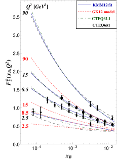
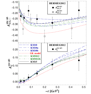
Figure 1: Left: The DIS structure function $F_{2}^{p}$ measurements Aid:1996au are confronted with the GK model (short–dashed), based on the next-to-leading order PDF parametrization CTEQ6M (dashed), the leading order PDF parametrization CTEQ6L1 (dot–dashed) as well as our DIS fit (solid) from Ref. Kumericki:2009uq . Right: Beam spin (upper panel) and beam charge (lower panel) asymmetry from the HERMES collaboration: measurements of $A^{\sin(\phi)}_{\rm LU,+}$ with the recoil detector (empty squares) Airapetian:2012pg and obtained from measurements of $A^{\sin(\phi)}_{\rm LU,I}$ and $A^{\cos(\phi)}_{\rm C}$ within the missing mass technique (filled squares) Airapetian:2009aa versus the GK model prediction (short–dashed) and various fits, KM10 (long-dashed), KM10a (dashed), KM10b (shorter dashed), KMM12 (dash–dotted), KMM12b (shorter dash–dotted), and KM15 (solid), to the HERMES data (filled squares) as solid curves.

On the other hand the GK model describes the asymmetry measurements of HERMES that were obtained within the missing mass technique, except for the beam spin asymmetry $A^{\sin(1\phi)}_{\rm LU}$, which is a key observable, compare full squares with short dashed line in the upper right panel of Fig. 1. On the other hand the recoil detector data of the HERMES collaboration (empty squares), which are consistent with the missing mass technique data, are described rather well by the GK model. Unfortunately, the two different data sets are not combined and the missing mass technique data suffer from a larger experimental uncertainty. As we will see in the next section the GK model quantitatively overestimates the beam spin asymmetry and the beam spin dependent cross section of JLab measurements.

2.2 Predictions of new JLab results and a new global fit

To fit globally the world data set of DVCS measurements from HERA and JLab collaborations, we employ a rather simple hybrid model. It is based on a double partial wave expansion for the sea-quark and gluon GPD, including the LO QCD evolution, and a dispersion integral representation for the valence quark content that does not evolve. Details of the model can be found in Kumericki:2009uq , and last published incarnation of the model (KMM12) Kumericki:2013br was obtained by a standard least-squares fitting procedure to the statistically independent set of 95 DVCS data points. Total $\chi^{2}/n_{\rm d.o.f.}$ was 123.5/80, where most problematic data was (i) HERMES data with longitudinally polarized target (and to some extent beam), and (ii) the very precise Hall A cross-section data (especially $t$-dependence of the first cosine harmonic).

On Table 1 we list all data used in fits, as well as $\chi^{2}/n_{\rm pts}$ values for particular datasets, for the KMM12 model, and for the new KM15 model to be discussed below. To give additional information about compatibility of the fit with the data, we list also the values of the “pull” of each dataset, defined for dataset consisting of $N$ measurements as

$$\text{pull}\equiv\frac{1}{\sqrt{N}}\sum_{i=1}^{N}\frac{f(x_{i})-y_{i}}{\Delta y_{i}}\;,$$ (11)

where $f(x_{i})$ is model value for a given kinematics $x_{i}$, while $y_{i}$ and $\Delta y_{i}$ are the corresponding experimental value and uncertainty, respectively. For a perfect model, pull (11) would be a random variable distributed according to a Gaussian distribution with zero mean and unit standard deviation.

Table 1: Observables used for KMM12 and KM15 fits, together with corresponding values of $\chi^{2}/n_{\rm pts}$ and “pulls” (11).

Collaboration	Observable	Ref.	$n_{\rm pts}$	KMM12			KM15
				$\chi^{2}/n_{\rm pts}$	pull		$\chi^{2}/n_{\rm pts}$	pull
ZEUS	$\sigma_{\rm DVCS}$	Chekanov:2008vy ; Chekanov:2003ya	11	0.49	-1.76		0.51	-1.74
ZEUS,H1	$d\sigma_{\rm DVCS}/dt$	Aaron:2009ac ; Chekanov:2008vy ; Aktas:2005ty	24	0.97	0.85		1.04	1.37
HERMES	$A_{\rm C}^{\cos 0\phi}$	Airapetian:2012mq	6	1.31	0.49		1.24	0.29
HERMES	$A_{\rm C}^{\cos\phi}$	Airapetian:2012mq	6	0.24	-0.56		0.07	-0.20
HERMES	$A_{\rm LU,I}^{\sin\phi}$	Airapetian:2012mq	6	2.08	-2.52		1.34	-1.28
CLAS	$A_{\rm LU}^{\sin\phi}$	Girod:2007aa	4	1.28	2.09
CLAS	$A_{\rm LU}^{\sin\phi}$	Gavalian:2008aa ; Pisano:2015iqa	13				1.24	0.63
CLAS	$\Delta\sigma^{\sin\phi,w}$	Jo:2015ema	48				0.41	-1.66
CLAS	$d\sigma^{\cos 0\phi,w}$	Jo:2015ema	48				0.16	-0.21
CLAS	$d\sigma^{\cos\phi,w}$	Jo:2015ema	48				1.16	6.36
Hall A	$\Delta\sigma^{\sin\phi,w}$	Munoz_Camacho:2006hx	12	1.06	-2.55
Hall A	$d\sigma^{\cos 0\phi,w}$	Munoz_Camacho:2006hx	4	1.21	2.14
Hall A	$d\sigma^{\cos\phi,w}$	Munoz_Camacho:2006hx	4	3.49	-0.26
Hall A	$\Delta\sigma^{\sin\phi,w}$	Defurne:2015kxq	15				0.81	-2.84
Hall A	$d\sigma^{\cos 0\phi,w}$	Defurne:2015kxq	10				0.40	0.92
Hall A	$d\sigma^{\cos\phi,w}$	Defurne:2015kxq	10				2.52	-2.42
HERMES,CLAS	$A_{\rm UL}^{\sin\phi}$	Airapetian:2010ab ; Chen:2006na	10	1.90	-1.89		1.10	-1.94
HERMES	$A_{\rm LL}^{\cos 0\phi}$	Airapetian:2010ab	4	3.44	2.17		3.19	1.99
HERMES	$A_{\rm UT,I}^{\sin(\phi-\phi_{S})\cos\phi}$	Airapetian:2008aa	4	0.90	0.61		0.90	0.71
CLAS	$A_{\rm UL}^{\sin\phi}$	Pisano:2015iqa	10				0.76	0.38
CLAS	$A_{\rm LL}^{\cos 0\phi}$	Pisano:2015iqa	10				0.50	-0.22
CLAS	$A_{\rm LL}^{\cos\phi}$	Pisano:2015iqa	10				1.54	2.40

Table 2: Valence (top) and sea quark (bottom) related hybrid model parameters, as obtained by the global DVCS fit KM15 to 290 data points with $\chi^{2}/{\rm d.o.f.}=240./275$. For detailed description of the model and parameters see Refs. Kumericki:2013br ; Kumericki:2009uq . Parameters of the old KMM12 fit Kumericki:2013br are also given for comparison.

	$M^{\rm val}$	$r^{\rm val}$	$b^{\rm val}$	$C$	$M_{C}$	$\tilde{M}^{\rm val}$	$\tilde{r}^{\rm val}$	$\tilde{b}^{\rm val}$	$r_{\pi}$	$M_{\pi}$
KM15	0.789	0.918	0.4	2.768	1.204	3.993	0.881	0.4	2.646	4.
KMM12	0.95	1.12	0.4	1.	2.08	3.52	1.3	0.4	3.84	4.
	$(M^{\rm sea})^{2}$	$s_{2}^{\rm sea}$	$s_{4}^{\rm sea}$	$s_{2}^{\rm G}$	$s_{4}^{\rm G}$
KM15	0.482	1.071	-0.366	-2.991	0.905
KMM12	0.46	0.31	-0.14	-2.77	0.94

Adding 2015 JLab data to the world set, and refitting the same model, results in a model parameter values listed on Table 2. The key difference is brought by using 2015 Hall A cross section data instead of superseded 2006 one. Old and new Hall A data, and KMM12 and KM15 models are confronted on Fig. 2. One notices that the cross-section went down a bit and the strong $t$-dependence of the first cosine harmonic ($d\sigma^{\cos\phi,w}$, lowest panels) seen in 2006 data is significantly milder now. All this made possible the decrease of skewness parameters $r^{\rm val}$ and $\tilde{r}^{\rm val}$, i.e., the decrease of $\mathcal{H}$ and $\tilde{\mathcal{H}}$, as well as the decrease of the pion pole contribution, thus improving the fit of most of the other observables, see Table. 1. In particular, description of HERMES $A_{\rm LU,I}^{\sin\phi}$ is significantly improved, and overshooting (large positive pull) of CLAS $A_{\rm LU}^{\sin\phi}$ is not present any more.

Looking at longitudinally polarized target data, $\chi^{2}$ of $A_{\rm UL}^{\sin\phi}$ is also improved, while very large $\chi^{2}$ contribution of HERMES $A_{\rm LL}^{\cos 0\phi}$ is mostly due to a single outlier point so we don’t consider this a problem. First cosine harmonic of the cross section remains the most problematic observable to describe. As discussed above, in the Hall A case the tension is relaxed but still exists, and although $\chi^{2}$ value for new CLAS measurement is fine, the pull of 6.36 is unacceptably large, showing consistent overshooting of the data.

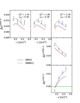
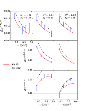
Figure 2: (Weighted) Fourier harmonics of Hall A 2006 Munoz_Camacho:2006hx (left) and 2015 Defurne:2015kxq (right) cross-section data, together with KMM12 (dashed) and KM15 (solid) models.

3 Local versus global extraction of CFFs

It is a standard problem in the phenomenology of scattering processes that if only an incomplete measurement is performed one can extract only certain combinations of squared helicity amplitudes at given kinematics. In the photon leptoproduction the interference between Bethe-Heitler bremsstrahlung process and deeply virtual Compton scattering offers various possibilities to access CFFs. To utilize the azimuthal angular dependence in the separation procedure, it is of advantage to perform first a Fourier analysis of the azimuthal angular dependence. In the following it is assumed that the eight sub-CFFs,

$${\cal F}\in\{\Im{\rm m}{\cal H},\Im{\rm m}{\cal E},\Im{\rm m}\widetilde{\cal H},\Im{\rm m}\widetilde{\cal E},\Re{\rm e}{\cal H},\Re{\rm e}{\cal E},\Re{\rm e}\widetilde{\cal H},\Re{\rm e}\widetilde{\cal E}\}\,,$$ (12)

appearing in LO and LT approximation (1) or, equivalently, in the hand-bag approach, dominate the twist-two associated first and zeroth asymmetry harmonics, where the latter one might be more contaminated by higher twist contributions than the former ones. Various methods for local extraction have been tested — we will discuss here only two: map of random numbers and a so-called quasi model-independent fitter code that is based on reference GPD models.

3.1 Mapping of random numbers

The mathematical problem to extract CFFs locally, i.e., at fixed values of $x_{\rm B}$, $Q^{2}$, and $t$, from experimental measurements, can be simply understood as a map from the space of observables into the space of CFFs Belitsky:2001ns . For asymmetry measurements with both kinds of leptons available this map of random numbers has been described in Ref. Kumericki:2013br . For cross section measurements with a polarized electron beam and/or polarized nucleon target it can be abstractly formulated as a set of linear and quadratic equations,

$$X \!\!\!=\!\!\! \mbox{\boldmath$b$}(F_{1},F_{2}|\mbox{\boldmath${\cal G}$})+\mbox{\boldmath$c$}^{-1}(F_{1},F_{2};\mbox{\boldmath${\cal G}$})\cdot\mbox{\boldmath$\cal F$}+\mbox{\boldmath$\cal F$}^{\dagger}\cdot\mbox{\boldmath$d$}\cdot\mbox{\boldmath$\cal F$}\,,\quad\mbox{\boldmath$X$}=\left(\begin{array}[]{c}X_{\rm unp}\\ \vdots\\ \vdots\\ X_{h_{n}S_{m}}\end{array}\right),\quad\mbox{\boldmath$\cal F$}=\left(\begin{array}[]{c}\Im{\rm m}H\\ \vdots\\ \Re{\rm e}H\\ \vdots\end{array}\right),$$ (21)

where the $n$-dimensional vector $X$ contains the experimental measurements of (weighted) harmonics at given kinematics, $\cal F$ is a $n$-dimensional vector of sub-CFFs (12) under the assumption that the remaining $24-n$ dimensional sub-CFF vector ${\cal G}$ can be considered as fixed. The constant vector

$$\mbox{\boldmath$b$}(F_{1},F_{2};\mbox{\boldmath${\cal G}$})=\mbox{\boldmath$b$}^{\rm BH}(F_{1},F_{2})+\mbox{\boldmath$b$}^{\rm INT}(F_{1},F_{2})\cdot\mbox{\boldmath${\cal G}$}+\mbox{\boldmath${\cal G}$}^{\dagger}\cdot\mbox{\boldmath$b$}^{\rm VCS}\cdot\mbox{\boldmath${\cal G}$}$$

contains contributions from the Bethe-Heitler term, interference term, and/or squared VCS amplitude, while the linear coefficient matrix $\mbox{\boldmath$c$}^{-1}(F_{1},F_{2};\mbox{\boldmath${\cal G}$})$ arises from the interference term and/or squared VCS amplitude. The (multi–valued) solution of the (quadratic) equations can be found by diagonalization.

Another local extraction method relies on the finding that apart from some power suppressed contributions, which are considered small, only certain linear and bilinear CFF combinations enter the interference term and the squared VCS amplitude, respectively. Strictly spoken, for each kinematical point we have different functional forms of these combinations which also depend on the center-of-mass energy or energy loss variable $y$. However, in the leading twist approximation the center-of-mass energy dependence approximately separates and Eq. (21) might be written as

$$X \!\!\!\approx\!\!\! \mbox{\boldmath$b$}(F_{1},F_{2})+\mbox{\boldmath$k$}^{-1}\cdot\mbox{\boldmath${\cal C}$}({\cal F}|F_{1},F_{2})+\mbox{\boldmath$K$}\cdot\mbox{\boldmath${\cal C}$}({\cal F}^{\dagger},\mbox{\boldmath$\cal F$})\,,$$ (22)

where now $\cal F$ contains the full set of (sub-)CFFs and $\mbox{\boldmath$k$}^{-1}$ and $K$ are matrices of dimensions $n$. For cross section measurements with an unpolarized nucleon target and a polarized electron beam Defurne:2015kxq ; Jo:2015ema the information which can be extracted are the first (weighted) harmonic of the beam helicity dependent cross section $\Delta(\phi)=\frac{1}{2}(d\sigma^{\uparrow}-d\sigma^{\downarrow})/dx_{\rm B}Q^{2}dtd\phi$,

$${\Delta}^{\sin(\phi)}\approx\frac{{\cal N}}{x_{\rm B}c^{\cal P}_{0}t}\frac{x_{\rm B}S_{++}(1)}{y}\Im{\rm m}{\cal C}_{\rm unp}^{{\cal I}}({\cal F})$$ (23a)

and zeroth and first (weighted) harmonics of the unpolarized cross section $$\Sigma(\phi)=\frac{1}{2}(d\sigma^{\uparrow}+d\sigma^{\downarrow})/dx_{\rm B}Q^{2}dtd\phi$$,

$${\Sigma}^{\cos(0\phi)}\approx\frac{{\cal N}}{x_{\rm B}c^{\cal P}_{0}t}\left[\frac{c^{\rm BH}_{0,{\rm unp}}}{\left(1+\epsilon^{2}\right)^{2}}+\frac{x_{\rm B}C_{++}(0)}{y}\Re{\rm e}{\cal C}_{\rm unp}^{{\cal I}}({\cal F})+\frac{2x_{\rm B}^{2}c^{\cal P}_{0}t}{Q^{2}}\frac{2-2y+y^{2}+\frac{\epsilon^{2}}{2}y^{2}}{1+\epsilon^{2}}\,{\cal C}_{\rm unp}^{\rm VCS}({\cal F},{\cal F}^{\ast})\right],$$ (23b)

$${\Sigma}^{\cos(\phi)}\approx\frac{-{\cal N}}{x_{\rm B}c^{\cal P}_{0}t}\left[\frac{c^{\rm BH}_{1,{\rm unp}}}{\left(1+\epsilon^{2}\right)^{2}}+\frac{x_{\rm B}C_{++}(1)}{y}\Re{\rm e}{\cal C}_{\rm unp}^{{\cal I}}({\cal F})+\frac{2w_{1}x_{\rm B}^{2}c^{\cal P}_{0}t}{Q^{2}}\frac{2-2y+y^{2}+\frac{\epsilon^{2}}{2}y^{2}}{1+\epsilon^{2}}\,{\cal C}_{\rm unp}^{\rm VCS}({\cal F},{\cal F}^{\ast})\right],$$ (23c)

allowing us to map directly the experimental data to the imaginary and real part of the CFF combination ${\cal C}_{\rm unp}^{{\cal I}}({\cal F})$ and the bilinear form ${\cal C}_{\rm unp}^{\rm VCS}({\cal F},{\cal F}^{\ast})$. For precise definition of various symbols see Ref. Belitsky:2012ch .

In the practical application of the strategy (21) one might straightforwardly calculate the sub-CFFs $\mbox{\boldmath$\cal F$}(\mbox{\boldmath$X$};F_{1},F_{2}|\mbox{\boldmath${\cal G}$})$, i.e., their mean and variance, as function of the experimental measurements, the form factor parametrization, and some given values of the remaining CFFs ${\cal G}$, whose fixed values can be varied in some model-dependent or theory-inspired region. Thus, the uncertainty of the extracted sub-CFFs $\mbox{\boldmath$\cal F$}(\mbox{\boldmath$X$};F_{1},F_{2}|\mbox{\boldmath${\cal G}$})$ contains essentially two main sources: the experimental uncertainty of the DVCS and the form factor measurements, including also the uncertainties of QED corrections, and the estimated uncertainty of the unknown CFF contributions. The strategy (22) has the advantages that within this assumption the uncertainties of the extracted linear and bilinear CFF combinations are governed only by the experimental uncertainties. However, some care is needed to have control over the uncertainties that are induced by the assumed approximation. A consistency check between the two methods is provided by evaluating the set of (approximate) equalities

$$\mbox{\boldmath${\cal C}$}({\cal F}|F_{1},F_{2})\approx\mbox{\boldmath${\cal C}$}(\mbox{\boldmath$\cal F$}(\mbox{\boldmath$X$};F_{1},F_{2}|\mbox{\boldmath${\cal G}$})|F_{1},F_{2})\,,\quad\mbox{\boldmath${\cal C}$}({\cal F}^{\dagger},\mbox{\boldmath$\cal F$})\approx\mbox{\boldmath${\cal C}$}(\mbox{\boldmath$\cal F$}^{\dagger}(\mbox{\boldmath$X$};F_{1},F_{2}|\mbox{\boldmath${\cal G}$}^{\dagger}),\mbox{\boldmath$\cal F$}(\mbox{\boldmath$X$};F_{1},F_{2}|\mbox{\boldmath${\cal G}$}))\,,$$ (24)

which have to be (almost) independent on the values of ${\cal G}$.

3.2 Quasi model-independent method based on reference GPD models

Another strategy, based on the method of least squares fitting, was suggested in Ref. Guidal:2008ie and utilized to locally extract GPD information in LO and LT approximation (1) from experimental measurements Guidal:2009aa ; Guidal:2010ig ; Guidal:2010de . Here, the parameters are eight multipliers, where their values are normalized to reference GPD predictions of the VGG code, reading here in our notation as

$$\Im{\rm m}{\cal F}(x_{\rm B},t,Q^{2})=a^{\Im{\rm m}}_{\cal F}\Im{\rm m}{\cal F}^{\rm VGG}(x_{\rm B},t,Q^{2})\,,\quad\Re{\rm e}{\cal F}(x_{\rm B},t,Q^{2})=a^{\Re{\rm e}}_{\cal F}\Re{\rm e}{\cal F}^{\rm VGG}(x_{\rm B},t,Q^{2})\,,$$ (25)

where ${\cal F}^{\rm VGG}$ are predicted by the VGG code via the convolution formula (1) and the multipliers $a^{\Im{\rm m}}_{\cal H},\cdots,a^{\Re{\rm e}}_{\widetilde{{\cal E}}}$ are the eight new model-independent fitting parameters. Further reduction might be made by setting some CFFs to zero, e.g., the imaginary part of the helicity non-conserved CFF $\widetilde{\cal E}$ whose smallness is suggested by the GPD findings in the DVMP analyses of $\pi^{+}$ electroproduction Bechler:2009me . Often the method was/is employed to an incomplete set of observables, i.e., the fitting problem is ill-posed and to reach convergency one constrains the seven parameters $|a^{\Im{\rm m}}_{\cal F}|\lesssim 5$ or so, including the more unreliable model estimates $|a^{\Re{\rm e}}_{\cal F}|\lesssim 5$ for the real part of CFFs. This method has been recently extended by generating an ensemble of fits with randomly distributed start values, where it is hoped that in this statistical manner also ill-posed fitting problems can be managed Boer:2014kya .

3.3 Comparison of results

Various strategies to locally extract CFFs from the almost over-complete DVCS asymmetry measurements of the HERMES collaboration were studied in Ref. Kumericki:2013br . Namely, one-to-one mapping, stepwise regression, and least squares fitting methods. The quasi model-independent method, see Sec. 3.2, utilizes all available harmonics, i.e., together with the stronger hypothesis that all observables are describable in the hand-bag approach noise is used to stabilize the fitting procedure. The results for $\{\Im{\rm m}{\cal H},\Im{\rm m}\widetilde{\cal H},\Re{\rm e}{\cal H}$} of Ref. Boer:2014kya are in good agreement with our findings Kumericki:2013br . Note that in Ref. Kumericki:2013br all local CFF values were reported, including the negative one for $\widetilde{\cal H}$ at $x_{\rm B}=0.08$, $Q^{2}=1.9\,{\rm GeV}^{2}$, and $-t=0.03\,{\rm GeV}^{2}$, however, we concluded that only the sub-CFFs $\Im{\rm m}{\cal H}$, $\Re{\rm e}{\cal H}$, $\Im{\rm m}\widetilde{\cal H}$, and maybe $\Im{\rm m}{\cal E}$ are accessible from HERMES measurements.

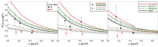
Figure 3: GPD $H$ (filled squares, slightly shifted to the l.h.s., and thick curves) and $\widetilde{H}$ (filled circles, slightly shifted to the r.h.s., and thin curves) from DVCS asymmetry measurements in three $\{x_{\rm B},Q^{2}\}$-bins versus $-t$ Pisano:2015iqa . They are locally extracted by the quasi model-independent method (squares and circles) Pisano:2015iqa , predicted by the GK model (dashed), KMM12 (dash-dotted) fit, KMM12b (shorter dash-dotted) fit, and from the new KM15 fit (solid).

The new CLAS beam spin asymmetry $A_{\rm LU}$ and longitudinally polarized target spin asymmetry $A_{\rm UL}$ and $A_{\rm LL}$ measurements Pisano:2015iqa were also analyzed with the quasi model-independent tool, shortly described in Sec. 3.2, were results for the imaginary parts of CFFs ${\cal H}$ and $\widetilde{\cal H}$ were presented in Fig. 25 of Ref. Pisano:2015iqa . In contrast to the HERMES analysis, there are only three asymmetries that are sensitive to two linear combinations (5) and (6) of the imaginary part of CFFs and one to the real part of Eq. (6), where in addition the normalization of asymmetries, i.e., the unpolarized cross section that is dominated by the Bethe-Heilter amplitude, is nonlinearly governed by all CFFs. We emphasise that CLAS data in the DVCS region do not indicate (apart from noise) the appearance of higher harmonics and that there might be some tension among longitudinal target spin asymmetry measurements from HERMES and CLAS collaborations. The results from the quasi model-independent approach have naturally large error bars, which provide a statistical representation of both the propagated experimental uncertainties and the model-dependent constraints on the non-extractable degree of freedom. As we would have expected, the locally extracted results in the DVCS kinematics are predicted from our older KMM12b and new KM15 fit (solid curves), shown for three DVCS bins in Fig. 3 while the GK (dashed) model prediction for GPD $H$ is too large. Note that all models have a rather similar GPD $\widetilde{H}$ prediction. The $t$-dependence of GPD $\widetilde{H}$ comes out flatter than for GPD $H$, which has a natural explanation in GPD models that incorporate form factor constraint. Namely, from the common GPD modeling and the fact that the axial nucleon form factor possesses a flatter $t$-dependence than the Pauli form factor, the above interpretation can be considered a model-dependent GPD prediction and only by means of the GPD framework one might loosely link the CFF $\widetilde{\cal H}$ to the axial-charge distribution, quantified by the axial form factor.

As explained in Sec. 3.1, the information which can be extracted from the new Hall A Defurne:2015kxq and CLAS Jo:2015ema cross section measurements are the imaginary and real parts of the CFF combination ${\cal C}_{\rm unp}^{{\cal I}}({\cal F})$ and the bilinear form ${\cal C}_{\rm unp}^{\rm VCS}({\cal F},{\cal F}^{\ast})$, see Eq. (23), while extraction of sub-CFFs is an ill-posed problem. We utilized the method (23), where uncertainties were added in quadrature and propagated via the transformation of the covariance matrix, see Kumericki:2013br . Note that in the propagation of experimental uncertainties we ignored the fact that systematic ones are asymmetric; however, for the purpose of an illustration at twist-two level this is not an important issue. Our results, shown as filled squares in the upper row of Fig. 4 coincide for the imaginary and real part of the linear combination ${\cal C}_{\rm unp}^{\cal I}$ and for the bilinear form ${\cal C}^{\rm VCS}$ with those that were obtained by the Hall A collaboration by fits to the $\phi$–dependent cross sections, see Fig. 22 of Ref. Defurne:2015kxq , where the net uncertainties are dominated by the systematic errors. The same method applied to the previous Hall A data Munoz_Camacho:2006hx , shown by empty squares, reveals some differences between the data sets (here we assume that these CFF combinations are smooth functions that vary only slightly within the small kinematical difference). However, as we will explain now, the adopted approximation implies an additional uncertainty and so the net errors of these results might be underestimated.

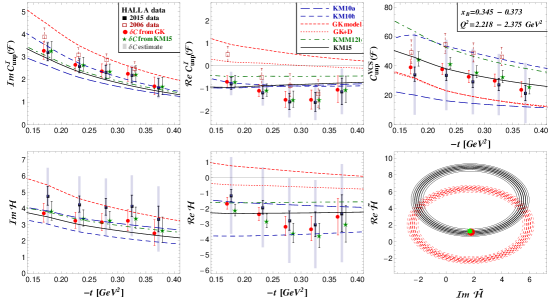
Figure 4: Upper row: imaginary part [left panel] and real part [middle panel] of the linear CFF combination ${\cal C}_{\rm unp}^{\cal I}({\cal F})$, defined in Eq. (5), as well as of the bilinear CFF combination ${\cal C}_{\rm unp}^{\rm VCS}({\cal F}^{\ast}_{\rm unp},{\cal F})$ [right panel] are mapped from the Hall A cross section measurements Defurne:2015kxq for Kin3 kinematics (8) within the Hall A approximation (filled squares) and utilizing the CFF ${\cal E}$ and $\widetilde{\cal E}$ values from the GK model (filled circles) and the KM15 fit (stars). The bands show the model uncertainties of power suppressed contributions in the range $|\Im{\rm m}{\cal E},\Im{\rm m}\widetilde{\cal H}|\leq 2$ and $|\Re{\rm e}{\cal E},\Re{\rm e}\widetilde{\cal H}|\leq 4$. The empty squares sketch the first Hall A measurements Munoz_Camacho:2006hx at slightly different kinematics. Lower row: possible region for $\Im{\rm m}{\cal H}$ [left panel] and $\Re{\rm e}{\cal H}$ [left panel] within the same CFF constraints as well as the 1-$\sigma$ ellipses for the $\widetilde{\cal H}$ constraint at $t=-0.232\,{\rm GeV}^{2}$ [right panel] for fixed CFF ${\cal E}$ and $\widetilde{\cal E}$ values taken from the GK model [dashed curves] and the KM15 fit [solid curves]. Model predictions are shown as curves, see Fig. 1. The dotted curves show a RDDA based GPD $H$, taken from the GK model, and the $D$-term form factor parametrization of Ref. Pasquini:2014vua .

On the other hand we might map the experimental data to the CFF ${\cal H}({\cal E},\widetilde{\cal H})$ and the bilinear form ${\cal C}^{\rm VCS}({\cal F}^{\ast},{\cal F})$ by utilizing the “exact” formulae for the restricted set of four CFFs. As expected, the extracted mean values for the linear combination

$$\Im{\rm m}{\cal C}_{\rm unp}^{\cal I}(\Delta|{\cal E}=\widetilde{\cal H}=0)\mbox{ \ and \ }\Re{\rm e}{\cal C}_{\rm unp}^{\cal I}(\Sigma|{\cal E}=\widetilde{\cal H}=0)$$

only slightly deviate from the findings within the direct extraction procedure in which power suppressed corrections are neglected. In average we find that the results deviate on the 0.2–0.3% level where the maximal deviation does not exceed 0.5% and 8% for the imaginary and real parts, respectively. Taking values for the unconstrained CFFs from the GK model prediction (filled circles) or our KM15 fit (stars) will only slightly change the mean values for this linear CFF combinations. In particular for the extraction of the bilinear form power suppressed corrections play a more important role and, thus, the two different methods provide results where in average the differences are $\sim 7\%$, however, can be up to $\sim 15\%$ in some bins. The results where the unconstrained CFFs ${\cal E}$, $\widetilde{\cal H}$, and $\widetilde{\cal E}$ are set to the GK model and the KM15 fit findings are shown as filled circles and stars, respectively. For both choices the values for $\widetilde{\cal H}$ are very similar and since the sensitivity to ${\cal E}$ is much more suppressed, we find rather similar results which are also very similar to those obtained in the ${\cal E}=\widetilde{\cal H}=0$ case. However, varying the unconstrained CFFs in the region

$$|\Im{\rm m}{\cal E},\Im{\rm m}\widetilde{\cal H}|\leq 2\mbox{ \ and \ }|\Re{\rm e}{\cal E},\Re{\rm e}\widetilde{\cal H}|\leq 4$$ (26)

generates for the real part of the linear combination and for the bilinear form a larger variation of the extracted mean values inside the gray rectangles, which reflects the importance of power suppressed contributions. Again the differences are much more pronounced for the extracted values of the bilinear CFF coefficient ${\cal C}_{\rm unp}^{\rm VCS}$. Taking into account this additional uncertainty, we can conclude that our previous KM10b (Kumericki:2011zc , dashed curves) and KMM12b (dash-dotted curves) fits in which only the relative $\phi$-modulation of the superseded dataset Munoz_Camacho:2006hx was utilized predicts the locally extracted values of the new data Defurne:2015kxq while the new global KM15 fit (solid curves) is entirely consistent with the locally extracted values. Compared to the older data set (empty squares), the GK model prediction (short dashed curves and dotted curves that adds a D-term contribution from Ref. Pasquini:2014vua ) gets more disfavored with respect to the new data set (filled squares).

Clearly, if one asks for the values of the CFF ${\cal H}$ the uncertainties depend much on the constraints for the remaining CFFs. This is illuminated in the first two panels of the lower row in Fig.  4 where due to the variation (26) the mean values of ${\cal H}({\cal E}=0,\widetilde{\cal H}=0)$ (filled squares) can move in the region of the rectangles. The findings for $\Im{\rm m}{\cal H}$ would be consistent with the values from the RDDA based GK model, however, taking values for $\widetilde{\cal H}$ and ${\cal E}$ from the GK model (circles) or the KM15 fit (stars) we realize that $\cal H$ is consistent with the KM15 fit and to some extent with our model predictions. In the right panel of the lower row we show the correlation between the real and imaginary part of the CFF $\widetilde{\cal H}$ within the 1-$\sigma$ band and with remaining CFFs fixed by the GK model (dashed curves) or the KM15 fit (solid curves). The model values for $\widetilde{\cal H}$ are again displayed as filled circle and star and one realizes that the GK  model violates this constraint while the KM15 fit respects it.

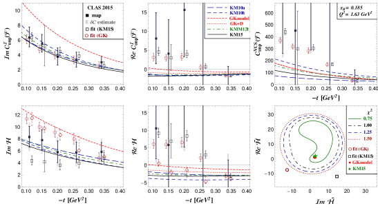
Figure 5: Imaginary [upper left panel] and real [middle panel] parts of linear CFF combination ${\cal C}^{\cal I}_{\rm unp}$ as well as the bilinear combination ${\cal C}^{\rm VCS}_{\rm unp}$ [upper right panel] for the $\{x_{\rm B}=0.185,Q^{2}=1.63\;{\rm GeV}^{2}\}$-bin are locally extracted from CLAS data Jo:2015ema by a map (filled squares), where rectangles show the variation of mean values by utilizing the constraint (26), and from a constrained four parameter, $\Im{\rm m}{\cal H}$, $\Im{\rm m}\widetilde{\cal H}$, $\Re{\rm e}{\cal H}$, $\Re{\rm e}\widetilde{\cal H}$, fit with start values from the GK model (empty circles) and KM15 fit (empty squares). Model predictions are shown as curves and are described in Fig. 4.

The CLAS collaboration used the quasi model-independent tool and tried to extract the CFF ${\cal H}$ from the cross section measurements Jo:2015ema , where only the two CFFs $\cal H$ and $\widetilde{\cal H}$ were taken as four fitting parameters. Apart from noise effects this is essentially a three parameter fit problem, see Eq. (23), where, however, four constrained parameters were used. We utilized a similar method, shown for the $\{x_{\rm B}=0.185,Q^{2}=1.63\;{\rm GeV}^{2}\}$-bin in Fig. 5 by the empty circles and squares. In the lower panel row we show that the resulting values, in particular for $\Im{\rm m}{\cal H}$ (left panel), might depend on the initial values and we might reproduce the CLAS result (see empty rhombi) if we take for the initial values the GK model predictions, however, we might find another solution if we utilize the KM15 result (empty squares) for the start values. Compared to our mapping procedure, providing us ${\cal H}({\cal E},\widetilde{\cal H})$ (filled squares and rectangles), the uncertainties from the fitting procedures are underestimated. The reason is that the unconstrained degrees of freedom tend to be on the boundary, see $t=-0.11\ {\rm GeV}^{2}$ example in the lower right panel, and thus the error propagation is not reliable. Such large values for $\widetilde{\cal H}$ can also be considered as inconsistent with the findings from the new CLAS asymmetry measurements, described above. Plugging our CFF fit results into the CFF combinations, see upper panel row, provides results that are consistent with our mapping procedure, however, the uncertainties from the fits might still be underestimated. Our model predictions and fit results are consistent with the CFF values from the map. In contrast to the CLAS statement, we conclude that the locally extracted ${\cal H}$ values disfavour a RDDA based GPD model (here the GK model).

4 Conclusions

We compared model predictions with the new DVCS measurements from the CLAS and Hall A collaborations where we utilize a (weighted) Fourier transform as filter to strengthen the discriminating power of predictions. We presented a new global DVCS fit KM15 showing that superseding 2006 Hall A cross section data with new one relieves some tensions, but description of first cosine harmonic of cross section remains imperfect. We showed that our global fit predictions KM10b and KMM12b, which ignored the normalization of the first Hall A cross section measurements, predict the new measurements reasonably well while a RDDA based model, e.g., the GK model, becomes more disfavored by the new data sets. These conclusions are partially in disagreement with the first analyses of the data by collaborations themselves. In particular, the new cross section measurements support the previous findings that even in fixed target kinematics such models provide a GPD $H$ that is too large. We further provided within our simple GPD ansatz from previous fits a good description of the new global DVCS data set and showed that the locally extracted CFF values are consistent with the global description. This analysis includes the GPD $\widetilde{H}$ which is rather compatible with RDDA based model predictions with respect to normalization and $t$-dependence which comes out flatter than for GPD $H$. Due to the new cross section measurements the indication that the GPD $H$ has a rather small skewness effect becomes more reliable.

We like to thank M. Guidal for a comparison of local fitting results that were obtained from our and his fitting analysis and we are indebted to H. Avakian, M. Garcon, and S. Niccolai for discussions. This work has been supported in part by the Croatian Science Foundation under the project number 8799, Croatian Ministry of Science, Education and Sport (MSES) under the NEWFELPRO grant agreement no. 54, and by the NRF of South Africa under CPRR grant no. 90509.

References

- (1) A.V. Belitsky, D. Müller, Y. Ji, Nucl.Phys. B878, 214 (2014), 1212.6674
- (2) J.J. Kelly, Phys. Rev. C70, 068202 (2004)
- (3) A.V. Belitsky, D. Müller, A. Kirchner, Nucl. Phys. B629, 323 (2002), hep-ph/0112108
- (4) S. Pisano et al. (CLAS), Phys. Rev. D91, 052014 (2015), 1501.07052
- (5) C.M. Camacho et al. (Jefferson Lab Hall A), Phys. Rev. Lett. 97, 262002 (2006), nucl-ex/0607029
- (6) M. Defurne et al. (Hall A) (2015), 1504.05453
- (7) H. Jo et al. (the CLAS) (2015), 1504.02009
- (8) P. Kroll, H. Moutarde, F. Sabatie, Eur.Phys.J. C73, 2278 (2013), 1210.6975
- (9) S.V. Goloskokov, P. Kroll, Eur. Phys. J. C53, 367 (2008), 0708.3569
- (10) M. Vanderhaeghen, P.A.M. Guichon, M. Guidal, Phys. Rev. D60, 094017 (1999), hep-ph/9905372
- (11) A. Freund, M. McDermott, M. Strikman, Phys. Rev. D67, 036001 (2003), hep-ph/0208160
- (12) J. Pumplin et al., JHEP 07, 012 (2002), hep-ph/0201195
- (13) S. Aid et al. (H1 Collaboration), Nucl.Phys. B470, 3 (1996), hep-ex/9603004
- (14) K. Kumerički, D. Müller, Nucl. Phys. B841, 1 (2010), 0904.0458
- (15) A. Airapetian et al. (HERMES), JHEP 1210, 042 (2012), 1206.5683
- (16) A. Airapetian et al. (HERMES), JHEP 11, 083 (2009), 0909.3587
- (17) K. Kumeric̀ki, D. Müller, M. Murray, Phys. Part. Nucl. 45, 723 (2014), 1301.1230
- (18) S. Chen et al. (CLAS), Phys. Rev. Lett. 97, 072002 (2006), hep-ex/0605012
- (19) S. Chekanov et al. (ZEUS), JHEP 05, 108 (2009), 0812.2517
- (20) S. Chekanov et al. (ZEUS), Phys. Lett. B573, 46 (2003), hep-ex/0305028
- (21) F. Aaron et al. (H1), Phys.Lett. B681, 391 (2009), 0907.5289
- (22) A. Aktas et al. (H1), Eur. Phys. J. C44, 1 (2005), hep-ex/0505061
- (23) A. Airapetian et al. (HERMES Collaboration), JHEP 1207, 032 (2012), 1203.6287
- (24) F.X. Girod et al. (CLAS), Phys. Rev. Lett. 100, 162002 (2008), 0711.4805
- (25) G. Gavalian et al. (CLAS), Phys. Rev. C80, 035206 (2009), 0812.2950
- (26) A. Airapetian et al. (HERMES), JHEP 06, 019 (2010), 1004.0177
- (27) A. Airapetian et al. (HERMES), JHEP 06, 066 (2008), 0802.2499
- (28) M. Guidal, Eur. Phys. J. A37, 319 (2008), 0807.2355
- (29) M. Guidal, H. Moutarde, Eur. Phys. J. A42, 71 (2009), 0905.1220
- (30) M. Guidal, Phys. Lett. B689, 156 (2010), 1003.0307
- (31) M. Guidal, Phys. Lett. B693, 17 (2010), 1005.4922
- (32) C. Bechler, D. Müller (2009), 0906.2571
- (33) M. Boör, M. Guidal, J. Phys. G42, 034023 (2015), 1412.4651
- (34) B. Pasquini, M. Polyakov, M. Vanderhaeghen, Phys.Lett. B739, 133 (2014), 1407.5960
- (35) K. Kumerički, T. Lautenschlager, D. Müller, K. Passek-Kumericki, A. Schaefer, M. Meskauskas (2011), 1105.0899