$L^{2}$-Kernels Of Dirac-Type Operators On Monopole Moduli Spaces

Abstract

We state some mathematical predictions concerning the kernels of Dirac-type operators on moduli spaces of (singular) monopoles in ${\mathbb{R}}^{3}$. These predictions follow from the semiclassical interpretation of physical results on spaces of (framed) BPS states in d=4, N=2 gauge theories.

MI-TH-1602

1 Introduction And Conclusion

The purpose of this note is to state some mathematical predictions for the differential geometry of moduli spaces of monopoles that follow from a semiclassical interpretation of some of the recent results on the BPS spectrum of four-dimensional gauge theories with N=2 supersymmetry. These predictions concern the nature of the $L^{2}$-kernel of a family of Dirac-type operators on moduli spaces of both singular and non-singular monopoles. We state three conjectures in Section §4. The first is a generalization of the famous conjecture of Ashoke Sen concerning the $L^{2}$-harmonic forms on monopole moduli space SegalSelby ; Sen:1994yi . The second and third conjectures describe the way in which the kernel is expected to jump as parameters in the family are continuously varied. We illustrate the conjectures with two examples in Section 5. In this note we only consider “pure” vectormultiplet theories and “pure” ’t Hooft line defects. The generalizations to theories with matter and general Wilson-’t Hooft line defects will appear elsewhere Brennan .

This note, aimed primarily at mathematicians, is a brief summary of the much more comprehensive paper MRV3 where the reader can find extended material explaining conventions, notation and background, as well as fuller explanations of the reasoning leading to the statements we make here. The papers Moore:2014jfa ; Moore:2014gua ; MRV3 also contain a more extensive list of references.

2 (Singular) Monopole Moduli Space

Let $G$ be a compact simple Lie group. Consider Yang-Mills-Higgs theory on ${\mathbb{R}}^{1,3}$ with action proportional to

$$\int_{{\mathbb{R}}^{1,3}}(F,*F)+(DX,*DX).$$ (1)

Here $(\cdot,\cdot)$ is a Killing form, normalized so the long-root has square-length $2$ and we have omitted the theta-term. (The latter is fully taken into account in MRV3 .) Magnetic monopoles are static solutions of the Yang-Mills-Higgs equations defined by solutions of the Bogomolnyi equations on ${\mathbb{R}}^{3}$

$$F=*_{3}DX$$ (2)

satisfying the following boundary conditions: We choose a regular element $X_{\infty}$ of the Lie algebra $\mathfrak{g}$ of $G$. This selects a Cartan subalgebra $\mathfrak{t}$ as well as a system of simple roots $\alpha_{I}$, and coroots $H_{I}$, where $I$ runs from one to the rank of the group. In a suitable gauge we impose the asymptotic conditions as the radial distance $r$ from a choice of spatial origin goes to infinity:

$$\begin{split}X&=X_{\infty}-\frac{\gamma_{\mathrm{m}}}{2r}+\cdots\\ F&=\frac{1}{2}\gamma_{\mathrm{m}}\omega+\cdots\\ \end{split}$$ (3)

Here $\gamma_{\mathrm{m}}$ is the magnetic charge and the gauge bundle, restricted to spheres of constant radius $S^{2}_{r}$ for sufficiently large $r$, has a transition function on the equator $e^{{\rm i}\phi}\rightarrow e^{\gamma_{\mathrm{m}}\phi}$, so $\gamma_{\mathrm{m}}$ is in the coroot lattice $\Lambda_{\mathrm{cr}}$ of $\mathfrak{g}$, while $\omega=\sin\theta d\theta d\phi$ is a volume form on $S^{2}_{r}$. The moduli space of such solutions, identified by the group of gauge transformations that approach $1$ as $r\to\infty$ is denoted ${\cal M}(\gamma_{\mathrm{m}},X_{\infty})$ and is is a smooth hyperkähler manifold Atiyah:1988jp . Expanding $\gamma_{\mathrm{m}}=\sum_{I}n_{\mathrm{m}}^{I}H_{I}$, with $n_{\mathrm{m}}^{I}\in{\mathbb{Z}}$, the moduli space is nonempty iff all $n_{\mathrm{m}}^{I}$ are nonnegative and at least one is positive Taubes:1981gw , in which case the real dimension of the moduli space is $4\sum_{I}n_{\mathrm{m}}^{I}$ Weinberg:1979ma ; Weinberg:1979zt .

There is a Lie algebra of Killing vector fields on ${\cal M}(\gamma_{\mathrm{m}},X_{\infty})$ isomorphic to ${\mathbb{R}}^{3}\oplus\mathfrak{s}\mathfrak{o}(3)\oplus\mathfrak{t}$, the summands corresponding to symmetries of translation, rotation about the origin, and global gauge transformations, respectively. We define the Killing vector associated with an element $h\in\mathfrak{t}$ as follows. In a gauge $A_{0}=0$ let $\hat{A}=A_{i}dx^{i}+Xdx^{4}$ be a four-dimensional gauge field so that solutions of (2) are equivalent to self-dual gauge fields $\hat{A}$ that are translation invariant in $x^{4}$. Given such a solution solve $\hat{D}^{2}\epsilon=0$ for a smooth map $\epsilon:{\mathbb{R}}^{4}\to\mathfrak{g}$ that is translation invariant in $x^{4}$ and satisfies $\epsilon\to h$ for $r\to\infty$. Then the Killing vector ${\mathrm{G}}(h)$ has directional derivative at $\hat{A}$ given by $\frac{d}{ds}\hat{A}=-\hat{D}\epsilon$. The map $h\to{\mathrm{G}}(h)$ is a Lie algebra homomorphism from $\mathfrak{t}$ to the Lie algebra of triholomorphic Killing vectors of the universal cover $\widetilde{{\cal M}}(\gamma_{\mathrm{m}},X_{\infty})$ of ${\cal M}(\gamma_{\mathrm{m}},X_{\infty})$. In this paper we make the simplifying assumption that $n^{I}_{\mathrm{m}}>0$ for all $I$ so that the action is effective. (The more general situation is fully treated in MRV3 .) The universal cover is metrically a product

$$\widetilde{{\cal M}}(\gamma_{\mathrm{m}},X_{\infty})={\mathbb{R}}^{4}\times{\cal M}_{0}(\gamma_{\mathrm{m}},X_{\infty})$$ (4)

where the ${\mathbb{R}}^{4}$ factor has the standard Euclidean metric and is generated by the translation Killing vectors along with ${\mathrm{G}}(X_{\infty})$. The space ${\cal M}_{0}(\gamma_{\mathrm{m}},X_{\infty})$ is the “strongly centered” moduli space in the terminology of HitchinMantonMurray . The moduli space is a quotient ${\cal M}(\gamma_{\mathrm{m}},X_{\infty})=\widetilde{{\cal M}}(\gamma_{\mathrm{m}},X_{\infty})/\mathbb{D}$ where the group of Deck transformations $\mathbb{D}\cong{\mathbb{Z}}$, and is generated by an isometry $\phi$. An important point for us is that the group of hyperholomorphic isometries acting on the universal cover and defined by $\mathbb{D}_{\rm g}:=\{{\rm exp}[2\pi{\mathrm{G}}(h)]|h\in\Lambda_{\mathrm{mw}}\}$, is in general a proper subgroup of $\mathbb{D}$. Through any point $m_{0}\in{\cal M}(\gamma_{\mathrm{m}},X_{\infty})$ there is an orbit of the maximal torus defining a homomorphism $\pi_{1}(T,1)\to\pi_{1}({\cal M},m_{0})$. We may view this as a homomorphism $\mu:\Lambda_{\mathrm{mw}}\to{\mathbb{Z}}$. Based on the rational map formulation of monopole moduli spaces Atiyah:1988jp ; Donaldson ; Hurtubise ; Jarvis we prove that $\mu(\lambda)=(\gamma_{\mathrm{m}},\lambda)$ and for any $\lambda\in\Lambda_{\mathrm{mw}}$

$${\rm exp}[2\pi{\mathrm{G}}(\lambda)]=\phi^{\mu(\lambda)}.$$ (5)

The image of $\mu$ is a subgroup $\ell{\mathbb{Z}}\subset{\mathbb{Z}}$ where $\ell$ is the positive integer such that $\ell^{-1}\gamma_{\mathrm{m}}^{\vee}\in\Lambda_{\mathrm{rt}}$ is primitive. (Equivalently, it is the gcd of the components of $\gamma_{\mathrm{m}}^{\vee}$ along a basis of simple roots.)

We now allow singularities in the monopole field corresponding, physically, to the introduction of an ’t Hooft line defect at the origin. The data of the singularity is given by (the Weyl orbit of) an element $P$ of the cocharacter lattice $\Lambda_{G}={\rm Hom}(U(1),T)$ where $T$ is the Cartan torus of $G$ with Lie algebra $\mathfrak{t}$. Singular monopoles satisfy equation (2), together with boundary conditions (3) for $r\to\infty$ along with the boundary conditions that read, in a suitable gauge,

$$\begin{split}X&=-\frac{P}{2r}+{\cal O}(r^{-1/2})\\ F&=\frac{1}{2}P\omega+{\cal O}(r^{-3/2})\\ \end{split}$$ (6)

for $r\to 0$. The space of solutions to (2),(3),and (6), quotiented by gauge transformations approaching $1$ at $r\to\infty$ and the normalizer of $P$ for $r\to 0$, is the moduli space $\overline{\underline{{\cal M}}}(P,\gamma_{\mathrm{m}},X_{\infty})$. It is a hyperkähler manifold with singularities on codimension four loci. The singularities are due to the phenomenon of monopole bubbling Kapustin:2006pk ; Moore:2014gua and in some cases are loci of orbifold singularities. Let

$$\tilde{\gamma}_{\mathrm{m}}:=\gamma_{\mathrm{m}}-P^{-}=\sum_{I}\tilde{n}^{I}_{\mathrm{m}}H_{I}$$ (7)

where $P^{-}$ is the Weyl image of $P$ in the chamber with $\langle\alpha_{I},P\rangle\leq 0$ for all $I$. It is conjectured in Moore:2014jfa (with some supporting evidence given in Moore:2014gua ) that the moduli space is nonempty iff $\tilde{n}^{I}_{\mathrm{m}}\geq 0$. The presence of the singularity at the spatial origin reduces the Lie algebra of Killing vectors to $\mathfrak{s}\mathfrak{o}(3)\oplus\mathfrak{t}$. The space $\overline{\underline{{\cal M}}}(P,\gamma_{\mathrm{m}},X_{\infty})$ only depends on the Weyl group orbit $[P]$ of $P$, up to hyperkähler isometry.

3 Consequences of $N=2$ Supersymmetry

3.1 General Remarks

We now consider the above Yang-Mills-Higgs theory in the context of N=2 supersymmetric gauge theory. The requirement of N=2 supersymmetry brings in a number of new features. (See Weinberg:2006rq for a comprehensive review.)

The first new feature is the presence of a second adjoint Higgs field $Y$. The Hamiltonian contains a potential energy term proportional to $\int_{{\mathbb{R}}^{3}}([X,Y],*[X,Y])$ and this term forces finite energy field configurations to obey $Y\to Y_{\infty}$ for $r\to\infty$ with $Y_{\infty}\in\mathfrak{t}$.

A second new feature is the existence in the quantum theory of distinguished quantum mechanical states known as “BPS states” Witten:1978mh ; Seiberg:1994rs . These are quantum mechanical analogs of the classical dyon field configurations satisfying the Bogomolnyi bound, and indeed the latter configurations are semiclassical approximations to BPS states at weak coupling. On the Coulomb branch of vacua of the N=2 quantum field theory the gauge group is broken down to the maximal torus $T$ and the BPS states carry electromagnetic charges with respect to this unbroken gauge symmetry. In the semiclassical limit there is a distinguished duality frame and the electromagnetic charge $\gamma$ is valued in the lattice

$$\Gamma:=\Lambda_{\mathrm{mw}}\oplus\Lambda_{\mathrm{wt}}\subset\mathfrak{t}\oplus\mathfrak{t}^{\vee}.$$ (8)

The lattice $\Gamma$ has a natural symplectic form defined by

$$\llangle\gamma_{1},\gamma_{2}\rrangle=\llangle\gamma_{1,\mathrm{m}}\oplus\gamma^{\mathrm{e}}_{1},\gamma_{2,\mathrm{m}}\oplus\gamma^{e}_{2}\rrangle:=\langle\gamma^{\mathrm{e}}_{1},\gamma_{2,\mathrm{m}}\rangle-\langle\gamma^{e}_{2},\gamma_{1,\mathrm{m}}\rangle.$$ (9)

It is valued in $\frac{1}{\mathpzc{z}}{\mathbb{Z}}$, where $\mathpzc{z}$ is the order of the center of the universal cover $\widetilde{G}$.

A third new feature is that the ’t Hooft line defects can be generalized to line defects preserving four out of the eight supersymmetries. In the physical theory the line defect depends on a choice of a further parameter, namely a phase $\zeta$ that determines which half-dimensional subspace of supersymmetries is preserved by the line defect. Since this parameter will not be visible in our mathematical predictions we will simply denote the line defect by $L([P])$. The insertion of a line defect changes the Hilbert space, but, when singularities at the origin are properly taken into account one can still define a Bogomolnyi bound. The so-called framed BPS states are the BPS states in the presence of a supersymmetric line defect Gaiotto:2010be . They have electromagnetic charge $\gamma$ in the $\Gamma$-torsor $\left(P+\Lambda_{\mathrm{cr}}\right)\oplus\Lambda_{\mathrm{rt}}$.

A fourth new feature arising from N=2 supersymmetry is that low energy excitations of (singular) monopoles (the dynamics of “collective coordinates”) are described by supersymmetric quantum mechanics on moduli space Manton:1981mp ; Gauntlett:1993sh ; Gauntlett:1995fu ; Gauntlett:1999vc ; Weinberg:2006rq . The paper MRV3 has an in-depth review of these results, including generalizations accounting for the effects of a theta angle, the presence of singular monopoles, and the inclusion of one-loop effects.

3.2 Geometrical Definitions Of BPS States

The supersymmetric dynamics of collective coordinates leads to geometrical definitions of the spaces of BPS states. For brevity we henceforth denote ${\cal X}:=X_{\infty}$ and ${\cal Y}:=Y_{\infty}$.

We begin with the framed BPS states. Let $\not{D}^{\cal Y}$ be the Dirac-type operator on the bundle of $L^{2}$-normalizable Dirac spinors on $\overline{\underline{{\cal M}}}(P,\gamma_{\mathrm{m}};{\cal X})$ defined by $\not{D}^{\cal Y}=\not{D}+\not{{\mathrm{G}}}({\cal Y})$, where $\not{D}$ is the standard Dirac operator and $\not{{\mathrm{G}}}({\cal Y})$ is Clifford multiplication by the one-form derived from the triholomorphic Killing vector ${\mathrm{G}}({\cal Y})$. For brevity, in what follows we will simply refer to $\not{D}^{\cal Y}$ as a “Dirac operator.”

Definition: The space of semiclassical framed BPS states, in the vacuum $({\cal X},{\cal Y})$, in the presence of the supersymmetric defect $L([P])$, and which have magnetic charge $\gamma_{\mathrm{m}}\in P+\Lambda_{\mathrm{cr}}$, is:

$${\rm ker}_{L^{2}}(\not{D}^{\cal Y}).$$ (10)

The reason for the phrase “in the vacuum $({\cal X},{\cal Y})$” is explained in Remark 2 below. In the semiclassical description the magnetic charge of the BPS states is encoded in the choice of moduli space $\overline{\underline{{\cal M}}}(P,\gamma_{\mathrm{m}};{\cal X})$ whereas the electric charge is the character of the triholomorphic action of $\mathfrak{t}$ on ${\rm ker}_{L^{2}}(\not{D}^{\cal Y})$. Indeed, we can define the spaces of framed BPS states of fixed electromagnetic charge $\gamma=\gamma_{\mathrm{m}}\oplus\gamma^{\mathrm{e}}$ from the isotypical decomposition with respect to the action of $\mathfrak{t}$:

$${\rm ker}_{L^{2}}(\not{D}^{\cal Y})=\oplus_{\gamma^{\mathrm{e}}\in\Lambda_{\mathrm{wt}}}\overline{\underline{{\cal H}}}([P];\gamma;{\cal X},{\cal Y}).$$ (11)

A parallel definition can be given for the ordinary (“unframed” or “vanilla”) BPS states, but there are a two extra complications since one must “factor out the center of mass degrees of freedom” and then impose the proper equivariance condition with respect to the Deck group $\mathbb{D}$.

As preparation introduce the rank one projection operator $\textbf{P}:\mathfrak{t}\to\mathfrak{t}$ onto the line spanned by ${\cal X}$ and defined by $\textbf{P}(h):=\frac{(h,\gamma_{\mathrm{m}})}{({\cal X},\gamma_{\mathrm{m}})}{\cal X}$. Since P is a projection operator we have a direct sum decomposition:

$$\mathfrak{t}\cong{\rm Im}(\textbf{P})\oplus{\rm Im}(1-\textbf{P}):=\mathfrak{t}_{\mathrm{com}}\oplus\mathfrak{t}_{0}$$ (12)

of vector spaces. The subspace $\mathfrak{t}_{0}$ is the subspace orthogonal to $\gamma_{\mathrm{m}}$ in the Killing metric (but P is not the orthogonal projection in the Killing metric). In MRV3 we prove that for all $h\in\mathfrak{t}$,

$$({\mathrm{G}}(h),{\mathrm{G}}({\cal X}))=(h,\gamma_{\mathrm{m}}).$$ (13)

On the left hand side of this equation we use the hyperkähler metric on moduli space, and on the right hand side we use the Killing metric on $\mathfrak{t}$. Therefore, the orthogonal decomposition, using the hyperkähler metric, along $T{\mathbb{R}}^{4}\oplus T{\cal M}_{0}$ for the Killing vectors ${\mathrm{G}}(h)$ takes the form

$${\mathrm{G}}(h)={\mathrm{G}}(h_{\mathrm{com}})+{\mathrm{G}}(h_{0})$$ (14)

where, for any $h\in\mathfrak{t}$ we define $h_{\mathrm{com}}:=\textbf{P}(h)$ and $h_{0}:=(1-\textbf{P})(h)$. Now we can choose orthogonal coordinates $(x^{i},x^{4})$ for the ${\mathbb{R}}^{4}$ factor so that the three translation Killing vectors give translations in $x^{i}$ (holding all else fixed) and $\frac{\partial}{\partial x^{4}}$ is a vector field parallel to ${\mathrm{G}}({\cal X})$, normalized so that

$$(\frac{\partial}{\partial x^{4}},{\mathrm{G}}({\cal X})):=1$$ (15)

It follows from (5) that $\phi^{*}(x^{4})=x^{4}+2\pi$.

We now split the Dirac operator $\not{D}^{\cal Y}$ on $\widetilde{{\cal M}}(\gamma_{\mathrm{m}},X_{\infty})$ using the splitting of the tangent bundle following from (4):

$$\not{D}^{{\cal Y}}=\not{D}^{{\cal Y}}_{\rm com}+\not{D}^{{\cal Y}}_{0}.$$ (16)

Explicitly, in terms of the coordinates on ${\mathbb{R}}^{4}$ defined above we have

$$\not{D}_{\mathrm{com}}^{{\cal Y}}=\Gamma^{i}\frac{\partial}{\partial x^{i}}+\Gamma^{4}\left(\frac{\partial}{\partial x^{4}}-{\rm i}\frac{({\cal Y},\gamma_{\mathrm{m}})}{({\cal X},\gamma_{\mathrm{m}})}\right)$$ (17)

where $\Gamma^{i},\Gamma^{4}$ are $4\times 4$ gamma matrices. We now define subspaces of sections of spinor bundles:

$${\cal K}_{\mathrm{com}}:={\rm ker}\not{D}_{\mathrm{com}}^{{\rm Y}^{\prime}}\subset\Gamma[{\cal S}\to{\mathbb{R}}^{4}]$$ (18)

$${\cal K}_{0}:={\rm ker}_{L^{2}}\not{D}_{0}^{{\rm Y}}\subset\Gamma_{L^{2}}[{\cal S}\to{\cal M}_{0}]$$ (19)

with ${\rm Y}^{\prime}\in\mathfrak{t}_{\mathrm{com}}$ and ${\rm Y}\in\mathfrak{t}_{0}$. By pulling back from the two factors and multiplying we get a subspace of sections of the spinor bundle on $\widetilde{{\cal M}}$:

$${\cal K}:=\pi_{\mathrm{com}}^{*}({\cal K}_{\mathrm{com}})\otimes\pi_{0}^{*}({\cal K}_{0})$$ (20)

and ${\cal K}$ is annihilated by $\not{D}^{{\cal Y}}$ for ${\cal Y}={\rm Y}^{\prime}+{\rm Y}$. There are no $L^{2}$-harmonic spinors on ${\mathbb{R}}^{4}$ for $\not{D}^{{\cal Y}}_{\rm com}$. This is physically reasonable since the monopoles are particles and definite momentum eigenstates are plane waves. On the other hand, we do not wish to have such continuous degrees of freedom “internally” so it is important to impose the $L^{2}$ condition in the definition of ${\cal K}_{0}$.

Now, ${\cal K}$ is a representation of $\mathfrak{t}$ and we can decompose it into eigenspaces of charge $\gamma^{\mathrm{e}}\in\mathfrak{t}^{\vee}$. Let ${\cal G}(h)$ denote the lift of the diffeomorphism ${\rm exp}[2\pi{\mathrm{G}}(h)]$ to the spinor bundle. (It exists.) By definition, a “spinor of electric charge $\gamma^{\mathrm{e}}\in\mathfrak{t}^{\vee}$” is one such that for all $h\in\mathfrak{t}$:

$${\cal G}(h)^{*}\Psi={\rm exp}[-2\pi{\rm i}\langle\gamma^{\mathrm{e}},h\rangle]\Psi.$$ (21)

The general element $\Psi_{\mathrm{com}}\in{\cal K}_{\mathrm{com}}$ is of the form $\Psi_{\mathrm{com}}=e^{-{\rm i}qx^{4}}s$, where $s\in\mathbb{C}^{4}$ is a constant Dirac spinor and $q=-({\cal Y},\gamma_{\mathrm{m}})/({\cal X},\gamma_{\mathrm{m}})$. On the other hand, the $\mathfrak{t}$-action on ${\cal K}$ factors through a product of a $\mathfrak{t}_{\mathrm{com}}$ action on ${\cal K}_{\mathrm{com}}$ and a $\mathfrak{t}_{0}$-action on ${\cal K}_{0}$. It follows that we must also have

$$q=\frac{\langle\gamma^{\mathrm{e}},{\cal X}\rangle}{(\gamma_{\mathrm{m}},{\cal X})}$$ (22)

and hence

$$({\cal Y},\gamma_{\mathrm{m}})+\langle\gamma^{\mathrm{e}},{\cal X}\rangle=0$$ (23)

is a necessary condition for the existence of a spinor in ${\cal K}$ with the data $({\cal X},{\cal Y},\gamma_{\mathrm{m}},\gamma^{\mathrm{e}})$.

A spinor $\Psi\in{\cal K}$ will only descend to ${\cal M}(\gamma_{\mathrm{m}},{\cal X})$ if $\gamma^{\mathrm{e}}$ is properly quantized, that is, if $\gamma^{\mathrm{e}}\in\Lambda_{\mathrm{mw}}^{\vee}=\Lambda_{\mathrm{rt}}$. However, because of equation (5) we must impose a further invariance condition under a cyclic group ${\mathbb{Z}}/\ell{\mathbb{Z}}$. Thus the physically relevant kernel of the Dirac operator is

$$\left(\oplus_{\gamma^{\mathrm{e}}\in\Lambda_{\mathrm{rt}}}{\cal K}^{\gamma^{\mathrm{e}}}\right)^{{\mathbb{Z}}/\ell{\mathbb{Z}}}$$ (24)

and since $\phi$ commutes with the $\mathfrak{t}$ action we may impose the cyclic group invariance on each isotypical summand. We define (24) to be the space of semiclassical BPS states in the vacuum $({\cal X},{\cal Y})$, with magnetic charge $\gamma_{\mathrm{m}}$. Since ${\cal K}_{\mathrm{com}}\cong\mathbb{C}^{4}$ we may factor it out of (24) and define both the space of BPS states and the “internal BPS states” by

$$({\cal K}^{\gamma^{\mathrm{e}}})^{{\mathbb{Z}}/\ell{\mathbb{Z}}}:={\cal H}(\gamma;{\cal X},{\cal Y}):={\cal K}_{\mathrm{com}}\otimes{\cal H}_{0}(\gamma;{\cal X},{\cal Y}).$$ (25)

We conclude this section with three remarks

1. The Killing vector fields arising from rotational symmetry around the origin are not triholomorphic. Nevertheless, they preserve the $L^{2}$-kernel of $\not{D}^{{\cal Y}}$ and $\not{D}^{{\cal Y}}_{0}$ on $\overline{\underline{{\cal M}}}$ and ${\cal M}_{0}$ respectively and hence the spaces $\overline{\underline{{\cal H}}}([P];\gamma;{\cal X},{\cal Y})$ and ${\cal H}_{0}(\gamma;{\cal X},{\cal Y})$ are representations of $\mathfrak{s}\mathfrak{o}(3)$. Moreover, the commutant $\mathfrak{s}\mathfrak{u}(2)$, in $\mathfrak{s}\mathfrak{o}(4N)$, of the $\mathfrak{s}\mathfrak{p}(N)$ holonomy (where we denote the real dimension of the moduli space $\overline{\underline{{\cal M}}}$ or ${\cal M}_{0}$ by $4N$) has a lift to the spinor bundle and again acts on the kernel of $\not{D}^{{\cal Y}}$. There is therefore an action of $\mathfrak{s}\mathfrak{o}(3)_{\rm rot}\oplus\mathfrak{s}\mathfrak{u}(2)_{R}$ on the BPS spaces. The subscripts indicate that the symmetry arises from rotational symmetry and “R-symmetry” in the physical theory.

2. We have referred to the pair $({\cal X},{\cal Y})$ as “defining a vacuum.” The precise translation to the physical Coulomb vacuum is described in full detail in MRV3 . In the framed case there are physical parameters $(u,\zeta)$, where $u$ is a point on the Coulomb branch and $\zeta$ is the phase mentioned above, and the mapping to $({\cal X},{\cal Y})$ is defined by

   $$\begin{split}{\cal X}&={\rm Im}(\zeta^{-1}a(u))\\ {\cal Y}&={\rm Im}(\zeta^{-1}a_{D}(u))\\ \end{split}$$ (26)

   where on the RHS we have used standard physical notations. The fiber of the mapping does not actually determine a unique vacuum: One can rescale $\zeta$ and $a$ by a common phase. In the unframed case the same formulae hold with $-\zeta$ replaced by the phase of the N=2 central charge $Z_{\gamma}(a)$. The standard collective coordinate supersymmetric quantum mechanics involves a potential energy term $\sim\parallel{\mathrm{G}}({\cal Y})\parallel^{2}$. Having a “moduli space with potential” is in fact a contradiction in terms; one is usually confined to working in a small potential energy approximation. In MRV3 it is suggested that (26) takes into account all the quantum corrections to the small potential energy approximation.

3. When hypermultiplet matter in a quaternionic representation $R$ of the gauge group is included the above definitions are extended by modifying the Dirac operator so that it also couples to the bundle associated to the universal bundle by the representation $R$. This bundle is endowed with a hyperholomorphic connection Manton:1993aa ; Gauntlett:1995fu ; Brennan .

3.3 Building BPS States From ${\cal K}_{0}$

A natural question to ask, and one which is important to our discussion of Fredholm conditions below, is whether spinors in the space ${\cal K}_{0}$ defined in (19) can be used to build BPS states in (25). In this section we describe those subspaces of ${\cal K}_{0}$. Accordingly, let us begin with the Dirac operator $\not{D}_{0}^{\rm Y}$ on ${\cal M}_{0}(\gamma_{\mathrm{m}},{\cal X})$ for an element ${\rm Y}\in\mathfrak{t}_{0}$. Only the subspace $\mathfrak{t}_{0}\subset\mathfrak{t}$ orthogonal to $\gamma_{\mathrm{m}}$ in the Killing metric will act effectively on ${\cal M}_{0}(\gamma_{\mathrm{m}},{\cal X})$ so our question becomes: When are spinors in the $\mathfrak{t}_{0}$-isotypical components of ${\cal K}_{0}$ factors of BPS spinors $\Psi\in{\cal H}(\gamma;{\cal X},{\cal Y})$ for some $\gamma^{\mathrm{e}}\in\Lambda_{\mathrm{rt}}$ and ${\cal Y}\in\mathfrak{t}$?

In order to answer this question introduce the rank one projection operator $\textbf{Q}:\mathfrak{t}^{\vee}\to\mathfrak{t}^{\vee}$ dual to P, i.e. $\langle\textbf{Q}(\gamma^{\mathrm{e}}),h\rangle:=\langle\gamma^{\mathrm{e}},\textbf{P}(h)\rangle$ for all $h\in\mathfrak{t}$. Then one computes $\textbf{Q}(\gamma^{\mathrm{e}})=\frac{\langle\gamma^{\mathrm{e}},{\cal X}\rangle}{(\gamma_{\mathrm{m}},{\cal X})}\gamma_{\mathrm{m}}^{\vee}$. Since Q is a projection operator we can use it to give a decomposition

$$\mathfrak{t}^{\vee}\cong{\rm Im}\textbf{Q}\oplus{\rm Im}(1-\textbf{Q}):=\mathfrak{t}_{\mathrm{com}}^{\vee}\oplus\mathfrak{t}_{0}^{\vee}$$ (27)

The isotypical decomposition of the $\mathfrak{t}_{0}$ action on ${\cal K}_{0}$ is a sum over characters $\gamma^{\mathrm{e}}_{0}\in\mathfrak{t}_{0}^{\vee}$. However, we can only complete a spinor $\Psi_{0}\in{\cal K}_{0}$ with a spinor $\Psi_{\mathrm{com}}\in{\cal K}_{\mathrm{com}}$ if the electric charge is properly quantized, and the condition for this is

$$\gamma^{\mathrm{e}}_{0}\in(1-\textbf{Q})(\Lambda_{\mathrm{rt}})~{}.$$ (28)

Let ${\cal L}(\gamma_{0}^{\mathrm{e}}):=\Lambda_{\mathrm{rt}}\cap(1-\textbf{Q})^{-1}(\gamma_{0}^{\mathrm{e}})$. For each choice of $\gamma^{\mathrm{e}}\in{\cal L}(\gamma_{0}^{\mathrm{e}})$ compute $q$ via (22), and form $\Psi=\Psi_{\mathrm{com}}\otimes\Psi_{0}$. Moreover, we define ${\rm Y}^{\prime}\in\mathfrak{t}_{\mathrm{com}}$ to be the solution to (23) and set ${\cal Y}:={\rm Y}^{\prime}+{\rm Y}$. We now have the quartet $({\cal X},{\cal Y},\gamma_{\mathrm{m}},\gamma^{\mathrm{e}})$ and $\Psi\in{\cal K}^{\gamma^{\mathrm{e}}}$ potentially describes a BPS state. However, we still must require that $\Psi$ descend from $\widetilde{{\cal M}}$ to ${\cal M}$. Recall that $\phi^{*}(x^{4})=x^{4}+2\pi$ and therefore we must require that

$$\phi^{*}(\Psi_{0})=e^{2\pi{\rm i}q}\Psi_{0}.$$ (29)

Now that we know when we can build BPS states from elements of ${\cal K}_{0}$ we should ask about uniqueness. Suppose that we have found an element of ${\cal L}(\gamma_{0}^{\mathrm{e}})$ so that (29) holds. What other charges in ${\cal L}(\gamma_{0}^{\mathrm{e}})$ will also support BPS states? Note that ${\cal L}(\gamma_{0}^{\mathrm{e}})$ is a torsor for $\Lambda_{\mathrm{rt}}\cap{\rm ker}(1-\textbf{Q})=\Lambda_{\mathrm{rt}}\cap{\rm Im}\textbf{Q}$ and since ${\rm Im}\textbf{Q}$ is just the real line through $\gamma_{\mathrm{m}}^{\vee}$ this is simply the set of multiples (necessarily rational) of $\gamma_{\mathrm{m}}^{\vee}$ that are in the root lattice. Therefore ${\cal L}(\gamma_{0}^{\mathrm{e}})\subset\Lambda_{\mathrm{rt}}$ is a ${\mathbb{Z}}$-torsor where the ${\mathbb{Z}}$-action is generated by $\gamma^{\mathrm{e}}\to\gamma^{\mathrm{e}}+\frac{1}{\ell}\gamma_{\mathrm{m}}^{\vee}$, that is, any two elements of the torsor are related by shifting

$$\gamma^{\mathrm{e}}\to\gamma^{\mathrm{e}}+\frac{k}{\ell}\gamma_{\mathrm{m}}^{\vee}$$ (30)

where $k$ is an integer. By (22) this has the effect of shifting: $q\to q+\frac{k}{\ell}$. Therefore, if (29) has a solution for some $\gamma^{\mathrm{e}}$ and we shift by integral multiples of $\gamma_{\mathrm{m}}^{\vee}$, that is, if $k$ is a multiple of $\ell$, then the same spinor $\Psi_{0}\in{\cal K}_{0}^{\gamma^{\mathrm{e}}_{0}}$ will satisfy (29) and hence we can use the same $\Psi_{0}$, but a different $\Psi_{\mathrm{com}}$, to construct a new BPS state. We call the collection of BPS states thus obtained a Julia-Zee tower. On the other hand, if we consider a shift (30) where $k$ is not a multiple of $\ell$ then the equivariance condition (29) changes. There might, or might not, be a different spinor in ${\cal K}_{0}^{\gamma^{\mathrm{e}}_{0}}$ transforming according to this new equivariance condition.

4 Mathematical Predictions

In this section we state three mathematical conjectures following from recent results in the physics literature.

4.1 Predictions From The No-Exotics Theorem

As we have remarked, the semiclassical spaces of framed and unframed BPS states:

$$\overline{\underline{{\cal H}}}([P];\gamma;{\cal X},{\cal Y}),$$

and ${\cal H}_{0}(\gamma;{\cal X},{\cal Y})$, respectively, are representations of $\mathfrak{s}\mathfrak{o}(3)_{\rm rot}\oplus\mathfrak{s}\mathfrak{u}(2)_{R}$. The “no exotics conjecture” of Gaiotto:2010be states that $\mathfrak{s}\mathfrak{u}(2)_{R}$ should act trivially on these spaces: They are direct sums of $\mathrm{SU}(2)_{R}$ singlets. This has been proven for gauge groups SU$(K)$ (using the relation of BPS states to the cohomology of spaces of representations of quivers and the Kontsevich-Soibelman wall-crossing formula) in Chuang:2013wt and for all simply laced gauge groups in DelZotto:2014bga . Recently a very beautiful general argument based on the structure of supersymmetric stress-tensor multiplets has been given CordovaDumitrescu . To see one simple implication for the Dirac operator we note that under the homomorphism

$${\rm SU}(2)_{R}\times{\rm Sp}(N)_{\rm hol}\rightarrow{\rm Spin}(4N)$$ (31)

the element $(-1,1)$ maps to the Clifford volume form with the natural orientation provided by any of the complex structures on the moduli space. It therefore follows that all the spinors in the kernel of the Dirac operator have positive chirality.

Moreover, choosing any complex structure on the moduli space we can express the no-exotics condition in terms of the Dolbeault operator acting on sections of $\Lambda^{0,*}$:

$$\bar{\partial}^{{\cal Y}}:=\bar{\partial}+{\mathrm{G}}({\cal Y})^{0,1}\wedge$$ (32)

using the isomorphism of the spinor bundle with $\Lambda^{0,*}$ HitchinHarmonicSpinors . In this formulation a set of generators of $\mathfrak{s}\mathfrak{u}(2)_{R}$ can be chosen so that

$$\begin{split}I^{3}|_{\Lambda^{0,q}}&=\frac{1}{2}(q-N)\textbf{1}\\ I^{+}=\upomega^{0,2}\wedge\qquad&\qquad I^{-}=\iota(\upomega^{2,0)})\\ \end{split}$$ (33)

By the no-exotics theorem these operators must act trivially on the cohomology and hence the $L^{2}$-cohomology of $H^{0,q}$ with respect to $\bar{\partial}^{{\cal Y}}$ (or at least that part satisfying the equivariance conditions with respect to the Deck transformation, as discussed above) is concentrated in the middle degree, $q=N$, and is primitive in the sense that it is annihilated by product with the $(0,2)$ combination of Kähler forms or by contraction with the $(2,0)$ combination of Kähler forms.

In ongoing work Brennan this discussion is generalized to include gauge theories with hypermultiplet matter. The $L^{2}$-cohomology of the corresponding operator $\bar{\partial}^{{\cal Y}}$ is still primitive and concentrated in the middle degree. In particular, specializing to $\mathfrak{g}=\mathfrak{s}\mathfrak{u}(2)$ with a hypermultiplet in the adjoint we obtain precisely the renowned prediction of Ashoke Sen Sen:1994yi based on $S$-duality.

4.2 Predictions From Wall-Crossing Formulae

We now consider the families of Dirac operators as we vary the Higgs fields. For simplicity our discussion will focus on the family parametrized by ${\cal Y}\in\mathfrak{t}$ in the framed case, and by ${\rm Y}\in\mathfrak{t}_{0}$ in the unframed case. Generically, $\not{D}^{{\cal Y}}$ acting on $L^{2}$ spinors over $\overline{\underline{{\cal M}}}(P,\gamma_{\mathrm{m}},{\cal X})$ (and $\not{D}_{0}^{\rm Y}$ acting on $L^{2}$ spinors over ${\cal M}_{0}(\gamma_{\mathrm{m}};{\cal X})$) is Fredholm, and by the no-exotics property, the character of ${\rm ker}\not{D}_{+}^{{\cal Y}}$ is the same as the character-valued index. Therefore, we expect the $\mathfrak{s}\mathfrak{o}(3)$ characters of $\overline{\underline{{\cal H}}}([P];\gamma;{\cal X},{\cal Y})$ and ${\cal H}_{0}(\gamma;{\cal X},{\cal Y})$ to be piecewise constant as functions of ${\cal Y}\in\mathfrak{t}$. However, on real codimension one walls, $\not{D}^{{\cal Y}}$, respectively $\not{D}_{0}^{\rm Y}$, will fail to be Fredholm. Physically, these walls correspond to walls of marginal stability, and using standard formulae for the $N=2$ central charges we are then led to the following predictions:

First, a translation of the standard criterion for crossing a wall of marginal stability, taking into account simplifications from working in the semiclassical limit, leads to the following criterion: $\not{D}_{0}^{\rm Y}$ is not Fredholm only if there are charges $\gamma_{1},\gamma_{2}\in\Gamma$, with $\gamma_{1,\mathrm{m}}+\gamma_{2,\mathrm{m}}=\gamma_{\mathrm{m}}$, “nonlocal” in the sense that $\llangle\gamma_{1},\gamma_{2}\rrangle\not=0$, and “occupied” in the sense that ${\cal H}(\gamma_{i};{\cal X},{\cal Y})\not=0$, for both $i=1,2$, where ${\cal Y}$ is constructed from ${\rm Y}$ and a choice of $\gamma^{\mathrm{e}}=\gamma^{\mathrm{e}}_{1}+\gamma^{\mathrm{e}}_{2}$ as described above. Note that (23) implies that

$$(\gamma_{i,\mathrm{m}},{\cal Y})+\langle\gamma_{i}^{\mathrm{e}},{\cal X}\rangle=0,\qquad\qquad i=1,2,$$ (34)

but these two equations are not independent of each other because their sum gives the identity (23) for the total charge $\gamma=\gamma_{1}+\gamma_{2}$. Indeed the the codimension wall on which $\not{D}_{0}^{\rm Y_{0}}$ will fail to be Fredholm (due to this pair of charges $\gamma_{1},\gamma_{2}$ ) is defined by (either) one of the above conditions, which can be written in the form:

$$({\rm Y},\gamma_{\mathrm{m},1})+\langle\gamma^{\mathrm{e}}_{1}-\gamma_{\mathrm{m},1}\frac{\langle\gamma^{\mathrm{e}},{\cal X}\rangle}{(\gamma_{\mathrm{m}},{\cal X})},{\cal X}\rangle=0.$$ (35)

Equation (35) defines a real codimension one wall in $\mathfrak{t}_{0}$. If ${\rm Y}$ crosses this wall the space ${\cal H}(\gamma;{\cal X},{\cal Y})$ will jump in a way dictated by the Kontsevich-Soibelman wall-crossing formula Kontsevich:2008fj . We expect that there is a relatively simple physical argument that shows that the continuous spectrum of $\not{D}_{0}^{\rm Y}$ extends down to zero at these real codimension one walls. It entails an analysis of the square of the operator $\not{D}_{0}^{\rm Y}$ using the asymptotic form of moduli space metrics discussed in Gibbons:1995yw ; Weinberg:2006rq . We hope to address this elsewhere.

Second, for singular monopoles, $\not{D}^{{\cal Y}}$ is Fredholm except on real codimension one walls defined by

$$W(\gamma_{\mathrm{h}}):=\{{\cal Y}:(\gamma_{\mathrm{h},\mathrm{m}},{\cal Y})+\langle\gamma_{\mathrm{h},\mathrm{e}},{\cal X}\rangle=0\quad\&\quad{\cal H}(\gamma_{\mathrm{h}};{\cal X},{\cal Y})\not=0\quad\&\quad Z_{\gamma_{\mathrm{h}}}(\zeta^{-1}a)<0\}$$ (36)

(The last condition $Z_{\gamma_{\mathrm{h}}}(\zeta^{-1}a)<0$ is satisfied automatically in the semiclassical region.) In this case a very explicit formula for the jump of $\overline{\underline{{\cal H}}}([P],\zeta;\gamma;{\cal X},{\cal Y})$ follows from Gaiotto:2010be : We introduce the Heisenberg group extension of $\mathbb{C}[\Gamma]$ defined by $X_{\gamma_{1}}X_{\gamma_{2}}=y^{\llangle\gamma_{1},\gamma_{2}\rrangle}X_{\gamma_{1}+\gamma_{2}}$ and form the generating function

$$F([P];{\cal X},{\cal Y}):=\sum_{\gamma\in\Gamma}{\overline{\underline{\Omega}}}([P],\gamma;{\cal X},{\cal Y})X_{\gamma}$$ (37)

where ${\overline{\underline{\Omega}}}(P,\gamma;{\cal X},{\cal Y})$ is the $\mathfrak{s}\mathfrak{o}(3)$ character of $\overline{\underline{{\cal H}}}([P];\gamma;{\cal X},{\cal Y})$, that is, the trace of $y^{2J}$ where $J$ is any generator of $\mathfrak{s}\mathfrak{o}(3)$ normalized to have half-integer eigenvalues. In a similar way, define a set of integers $a_{m}(\gamma_{\mathrm{h}})$ by the character of ${\cal H}(\gamma_{\mathrm{h}};{\cal X},{\cal Y})$, $\Omega(\gamma_{\mathrm{h}};{\cal X},{\cal Y})=\sum_{m}a_{m}(-y)^{m}$. Then, crossing a wall $W(\gamma_{\mathrm{h}})$ we have the transformation law $F\to SFS^{-1}$, where $S=\prod_{n>0}S_{n\gamma_{\mathrm{h}}}$,

$$S_{\gamma_{\mathrm{h}}}=\prod_{m}\Phi((-y)^{m}X_{\gamma_{\mathrm{h}}})^{a_{m}(\gamma_{\mathrm{h}})}$$ (38)

and $\Phi(X)=\prod_{k=1}^{\infty}(1+y^{2k-1}X)^{-1}$ is the quantum dilogarithm.

5 Two Examples

5.1 Example 1: Wall Crossing For Smooth Monopoles

We consider the case when $\mathfrak{g}$ has rank $2$, so there are two simple coroots and $\gamma_{\mathrm{m}}=H_{1}+H_{2}$. What follows is a reinterpretation of the discussion of Gauntlett:1999vc . In this case the strongly centered moduli space ${\cal M}_{0}$ is the Taub-NUT metric. We can represent it as projection $\pi:{\cal M}_{0}\to{\mathbb{R}}^{3}$ where the fiber is a circle, parametrized by $\uppsi\sim\uppsi+2\pi$, except for the fiber over the origin, which is just a point. Splitting ${\mathrm{G}}({\cal Y})$ to extract the component along ${\cal M}_{0}$ yields

$${\mathrm{G}}({\cal Y}_{0})=\frac{1}{\mathpzc{p}}(H_{1},{\cal Y}_{0})\frac{\partial}{\partial\uppsi}$$ (39)

where $\mathpzc{p}=1,2,3$ for $\mathfrak{g}=\mathfrak{s}\mathfrak{u}(3),\mathfrak{s}\mathfrak{o}(5),\mathfrak{g}_{2}$, respectively and we take $\alpha_{1}$ to be the long root. Electric charges of BPS states are of the form

$$\gamma^{\mathrm{e}}=n_{\mathrm{e}}^{1}\alpha_{1}+n_{\mathrm{e}}^{2}\alpha_{2}$$ (40)

with $n_{\mathrm{e}}^{1},n_{\mathrm{e}}^{2}\in{\mathbb{Z}}$. Now $\mathfrak{t}_{0}$ is one-dimensional and the projection in (28) is

$$\gamma^{\mathrm{e}}_{0}=(\mathpzc{p}n_{\mathrm{e}}^{1}-n_{\mathrm{e}}^{2})\cdot\left(\frac{m_{2}\alpha_{1}-m_{1}\mathpzc{p}\alpha_{2}}{\mathpzc{p}(m_{1}+m_{2})}\right)$$ (41)

where $m_{i}:=(H_{i},{\cal X})$. Define $N_{\mathrm{e},0}:=\mathpzc{p}n_{\mathrm{e}}^{1}-n_{\mathrm{e}}^{2}$. Then, for fixed $\gamma^{\mathrm{e}}_{0}$ the preimage of compatible electric charges is the ${\mathbb{Z}}$ torsor with fixed value of $N_{\mathrm{e},0}$, that is the set of electric charges $\gamma^{\mathrm{e}}=n\alpha_{1}+(n\mathpzc{p}-N_{\mathrm{e},0})\alpha_{2}$ with $n\in{\mathbb{Z}}$. Elements of ${\cal K}_{0}$ that can be used to build states of definite electric charge are equivariant in the $\uppsi$ direction: $L_{\frac{\partial}{\partial\uppsi}}\Psi_{0}=-{\rm i}N_{\mathrm{e},0}\Psi_{0}$. The non-Fredholm condition is now based on a pair of electromagnetic charges $\gamma_{i}=H_{i}\oplus n_{\mathrm{e}}^{i}\alpha_{i}$, $i=1,2$ with $\llangle\gamma_{1},\gamma_{2}\rrangle=-N_{\mathrm{e},0}\not=0$. The spaces ${\cal H}_{0}(\gamma_{i};{\cal X},{\cal Y})$ correspond to the case ${\cal M}_{0}={\rm pt}$ and are one-dimensional so the non-Fredholm criterion is satisfied. The jump in the $L^{2}$ kernel can be verified by direct computation in this case since the determination of the kernel of the Dirac-like operator $\not{D}_{0}^{\rm Y}$ on ${\cal M}_{0}$ is a computation going back to Pope:1978zx . The result is illustrated in Figure 1 and is simply the result predicted by the primitive wall-crossing formula of Denef:2007vg ; Diaconescu:2007bf , which suffices in this case since the $\gamma_{i}$ are primitive. Moreover, the boundstate wavefunction, as a function of the (suitably rescaled) radial direction $r$ in ${\mathbb{R}}^{3}$, is proportional to $r^{(|N_{\mathrm{e},0}|-1)/2}e^{-|2C+N_{\mathrm{e},0}|r}$ where ${\mathrm{G}}({\cal Y}_{0})=\frac{2\mu}{\mathpzc{p}^{2}}C\frac{\partial}{\partial\uppsi}$, $\mu^{-1}=m_{1}^{-1}+m_{2}^{-1}$, and the constant $C$ is proportional to the coordinate $y_{1}$ in Figure 1. The wavefunction is peaked at $r_{\rm ext}=|N_{\mathrm{e},0}|/|2C+N_{\mathrm{e},0}|$. This turns out to be precisely the bound-state radius computed from explicit BPS field configurations by Denef Denef:2002ru .

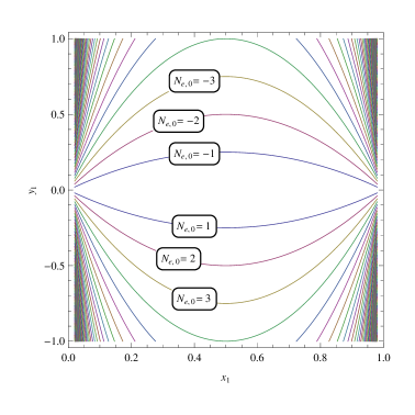
Figure 1: Walls of marginal stability for $\mathfrak{g}=\mathfrak{s}\mathfrak{u}(3),\mathfrak{s}\mathfrak{o}(5),\mathfrak{g}_{2}$ for $\mathpzc{p}=1,2,3$ respectively. We choose axes to be the scale-invariant quantities $x_{1}:=(H_{1},{\cal X})/(\gamma_{\mathrm{m}},{\cal X})$ and $y_{1}:=\mathpzc{p}(H_{1},{\cal Y}_{0})/(\gamma_{\mathrm{m}},{\cal X})$. The chamber containing the line $y_{1}=0$ has no BPS states. Crossing a wall labeled by $N_{\mathrm{e},0}$ in the direction away from the central chamber adds a tower of BPS states with electric charge $\gamma^{\mathrm{e}}=n\alpha_{1}+(\mathpzc{p}n-N_{\mathrm{e},0})\alpha_{2}$ with $n\in{\mathbb{Z}}$ to the spectrum. The $\mathfrak{s}\mathfrak{o}(3)_{\rm rot}$ representation ${\cal H}_{0}(\gamma;{\cal X},{\cal Y})$ gains a spin $j$ representation with $j=\frac{1}{2}(|N_{\mathrm{e},0}|-1)$. At the walls $x\to 0,1$ the classical mass of the monopoles goes to zero and the semiclassical analysis is not necessarily valid.

5.2 Example 2: Wall-Crossing For Singular Monopoles

We now consider $\mathfrak{g}=\mathfrak{s}\mathfrak{u}(2)$, but consider a singular monopole with $P=\frac{p}{2}H_{\alpha}$. We can take $p>0$. Splitting $\gamma=\gamma_{\mathrm{m}}\oplus\gamma^{\mathrm{e}}$ with $\gamma_{\mathrm{m}}=(\tilde{n}_{\mathrm{m}}-\frac{1}{2}p)H_{\alpha}$, we see that ${\overline{\underline{\Omega}}}(P,\gamma;{\cal X},{\cal Y})$ is the $\mathfrak{s}\mathfrak{o}(3)$ character of the Dirac operator on a moduli space of singular monopoles of dimension $4\tilde{n}_{\mathrm{m}}$. The spectrum of the ordinary BPS states is well-known Seiberg:1994rs : With our choice $p>0$ the only relevant spaces are ${\cal H}_{0}(\gamma_{n};{\cal X},{\cal Y})\cong\mathbb{C}$ with $\gamma_{n}=H_{\alpha}+n\alpha$. We can thus divide up the ${\cal Y}$-line into chambers separated by walls $W_{n}=W(\gamma_{n})$. In the chamber between walls $W_{n}$ and $W_{n+1}$ the generating function (37) is given by

$$F_{n}=\left[X_{1}^{-1/2}X_{2}^{-n/2}\left(U_{n}(f_{n})-X_{2}^{-1/2}U_{n-1}(f_{n})\right)\right]^{p}$$ (42)

where $X_{1}=X_{H_{\alpha}}$ and $X_{2}=X_{\alpha}$ generate the Heisenberg extension of $\mathbb{C}[\Gamma]$,

$$f_{n}:=\frac{1}{2}\left(X_{2}^{1/2}+X_{2}^{-1/2}\left(1+y^{2n+3}X_{1}X_{2}^{n+1}\right)\right),$$ (43)

and $U_{n}(\cos\theta)=\sin((n+1)\theta)/\sin\theta$. The result is proven in MRV3 by careful application of the wall crossing formula for $F([P];{\cal X},{\cal Y})$ and generalizes the result in Gaiotto:2010be at $y=1$. Equation (42) makes some fairly nontrivial predictions for $L^{2}$-kernels of Dirac operators on singular monopole moduli spaces, some of which are spelled out in detail in MRV3 .

References

- (1) M. F. Atiyah and N. J. Hitchin, “The Geometry And Dynamics Of Magnetic Monopoles. M.B. Porter Lectures,” Princeton University Press, 1988.
- (2) D. Brennan and G. Moore, work in progress
- (3) W. y. Chuang, D. E. Diaconescu, J. Manschot, G. W. Moore and Y. Soibelman, “Geometric engineering of (framed) BPS states,” Adv. Theor. Math. Phys. 18, 1063 (2014) [arXiv:1301.3065 [hep-th]].
- (4) C. Cordova and T. Dumitrescu, to appear.
- (5) M. Del Zotto and A. Sen, “About the Absence of Exotics and the Coulomb Branch Formula,” arXiv:1409.5442 [hep-th].
- (6) F. Denef, “Quantum quivers and Hall / hole halos,” JHEP 0210, 023 (2002) [hep-th/0206072].
- (7) F. Denef and G. W. Moore, “Split states, entropy enigmas, holes and halos,” JHEP 1111, 129 (2011) [hep-th/0702146].
- (8) E. Diaconescu and G. W. Moore, “Crossing the wall: Branes versus bundles,” Adv. Theor. Math. Phys. 14 (2010) [arXiv:0706.3193 [hep-th]].
- (9) Donaldson, S. K., “Nahm’s equations and the classification of monopoles,” Commun. Math. Phys. 96, 387-408 (1984)
- (10) D. Gaiotto, G. W. Moore and A. Neitzke, “Framed BPS States,” Adv. Theor. Math. Phys. 17, 241 (2013) [arXiv:1006.0146 [hep-th]].
- (11) J. P. Gauntlett, “Low-energy dynamics of N=2 supersymmetric monopoles,” Nucl. Phys. B 411, 443 (1994) [hep-th/9305068].
- (12) J. P. Gauntlett and J. A. Harvey, “S duality and the dyon spectrum in N=2 superYang-Mills theory,” Nucl. Phys. B 463, 287 (1996) doi:10.1016/0550-3213(96)00035-1 [hep-th/9508156].
- (13) J. P. Gauntlett, N. Kim, J. Park and P. Yi, “Monopole dynamics and BPS dyons N=2 superYang-Mills theories,” Phys. Rev. D 61, 125012 (2000) [hep-th/9912082].
- (14) G. W. Gibbons and N. S. Manton, “The Moduli space metric for well separated BPS monopoles,” Phys. Lett. B 356, 32 (1995) [hep-th/9506052].
- (15) N. Hitchin, “Harmonic spinors,” Advances in Math. 14 (1974) pp. 1-55.
- (16) N.J. Hitchin, N.S. Manton, M.K. Murray, “Symetric Monopoles,” arXiv:dg-ga/9503016
- (17) J. Hurtubise, “Monopoles and Rational Maps: A Note on a Theorem of Donaldson,” Commun. Math. Phys. 100, 191-196 (1985); J. Hurtubise, “The Classification of Monopoles for the Classical Groups,” Commun. Math. Phys. 120, 613-641 (1989); J. Hurtubise and M. Murray, “On The Construction of Monopoles for the Classical Groups,” Commun. Math. Phys. 122, 35-89 (1989)
- (18) S. Jarvis, “Euclidean Monopoles and Rational Maps,” Proc. London Math. Soc. (3) 77 (1998) 170-192; “Construction Of Euclidean Monopoles,” Proc. London Math. Soc. (3) 77 (1998) 193-214.
- (19) A. Kapustin and E. Witten, “Electric-Magnetic Duality And The Geometric Langlands Program,” Commun. Num. Theor. Phys. 1, 1 (2007) [hep-th/0604151].
- (20) M. Kontsevich and Y. Soibelman, “Stability structures, motivic Donaldson-Thomas invariants and cluster transformations,” arXiv:0811.2435 [math.AG].
- (21) N. S. Manton, “A Remark on the Scattering of BPS Monopoles,” Phys. Lett. B 110, 54 (1982). doi:10.1016/0370-2693(82)90950-9
- (22) N. S. Manton and B. J. Schroers, “Bundles over moduli spaces and the quantization of BPS monopoles,” Annals Phys. 225, 290 (1993). doi:10.1006/aphy.1993.1060
- (23) G. W. Moore, A. B. Royston and D. V. d. Bleeken, “Parameter counting for singular monopoles on ,” JHEP 1410, 142 (2014) [arXiv:1404.5616 [hep-th]].
- (24) G. W. Moore, A. B. Royston and D. Van den Bleeken, “Brane bending and monopole moduli,” JHEP 1410, 157 (2014) [arXiv:1404.7158 [hep-th]].
- (25) G. W. Moore, A. B. Royston and D. V. d. Bleeken, arXiv:1512.08924 [hep-th].
- (26) C. N. Pope, “Axial Vector Anomalies and the Index Theorem in Charged Schwarzschild and Taub - Nut Spaces,” Nucl. Phys. B 141, 432 (1978).
- (27) G. Segal and A. Selby, “The cohomology of the space of magnetic monopoles,” Comm. Math. Phys. 177 (1996), no. 3, 775–787.
- (28) N. Seiberg and E. Witten, “Electric - magnetic duality, monopole condensation, and confinement in N=2 supersymmetric Yang-Mills theory,” Nucl. Phys. B 426, 19 (1994) [Nucl. Phys. B 430, 485 (1994)] [hep-th/9407087].
- (29) A. Sen, “Dyon - monopole bound states, selfdual harmonic forms on the multi - monopole moduli space, and SL(2,Z) invariance in string theory,” Phys. Lett. B 329, 217 (1994) [hep-th/9402032].
- (30) M. Stern and P. Yi, “Counting Yang-Mills dyons with index theorems,” Phys. Rev. D 62, 125006 (2000) [hep-th/0005275].
- (31) C. H. Taubes, “The Existence of Multi - Monopole Solutions to the Nonabelian, Yang-Mills Higgs Equations for Arbitrary Simple Gauge Groups,” Commun. Math. Phys. 80, 343 (1981). doi:10.1007/BF01208275
- (32) E. J. Weinberg, “Parameter Counting for Multi-Monopole Solutions,” Phys. Rev. D 20, 936 (1979). doi:10.1103/PhysRevD.20.936
- (33) E. J. Weinberg, “Fundamental Monopoles and Multi-Monopole Solutions for Arbitrary Simple Gauge Groups,” Nucl. Phys. B 167, 500 (1980). doi:10.1016/0550-3213(80)90245-X
- (34) E. J. Weinberg and P. Yi, “Magnetic Monopole Dynamics, Supersymmetry, and Duality,” Phys. Rept. 438, 65 (2007) [hep-th/0609055].
- (35) E. Witten and D. I. Olive, “Supersymmetry Algebras That Include Topological Charges,” Phys. Lett. B 78, 97 (1978).