Character of Matter in Holography:
Spin-Orbit Interaction

Yunseok Seo¹, Keun-Young Kim², Kyung Kiu Kim^2,3 and Sang-Jin Sin¹

¹Department of Physics, Hanyang University
Seoul 133-791, Korea

²School of Physics and Chemistry, Gwangju Institute of Science and Technology,
Gwangju 500-712, Korea

³Department of Physics, College of Science, Yonsei University, Seoul 120-749, Korea

Abstract

Gauge/Gravity duality as a theory of matter needs a systematic way to characterise a system. We suggest a ‘dimensional lifting’ of the least irrelevant interaction to the bulk theory. As an example, we consider the spin-orbit interaction, which causes magneto-electric interaction term. We show that its lifting is an axionic coupling. We present an exact and analytic solution describing diamagnetic response. Experimental data on annealed graphite shows a remarkable similarity to our theoretical result. We also find an analytic formulas of DC transport coefficients, according to which, the anomalous Hall coefficient interpolates between the coherent metallic regime with $\rho_{xx}^{2}$ and incoherent metallic regime with $\rho_{xx}$ as we increase the disorder parameter $\beta$. The strength of the spin-orbit interaction also interpolates between the two scaling regimes. Keywords : Holography, Diamagnetism, DC conductivity, Anomalous Hall effect.
PACS numbers : 11.25.Tq, 72.15.Eb,

yseo@hanyang.ac.kr, fortoe@gist.ac.kr, kimkyungkiu@gmail.com, sangjin.sin@gmail.com

Overview and Summary: Recently, the gauge/gravity duality [1, 2, 3] attracted much interests as a possible candidate for a reliable method to calculate strongly correlated systems. It is a local field theory in one higher dimensional space called “bulk”, with a few classical fields coupled with anti deSitter(AdS) gravity. Since the strong coupling in the boundary, is dual to a weak coupling in the bulk, the bulk fields can be considered as local order parameters of a mean field theory in the bulk. It also provided a new mechanism for instabilities in gravity language[4] which is relevant to the superconductivity [5, 6] and the metal insulator transition [7]. However, as a theory for materials, it is still in lack of one essential ingradient, a way to distinguish one matter from the others. Although electron-electron interaction is traded for the gravity in the bulk, we still need to specify lattice-electron interactions to characterises the system. Without it, we would not know what system we are working for.

Naively one may try to introduce realistic lattice at the boundary to mimic the reality. However, its effects are mostly irrelevant in the infrared(IR) limit. In strong coupling limit where no quasiparticle exists, no fermi surface(FS) exists either. Actually in the absence of the FS, it is almost impossible to write down any relevant interaction term in a local field theory in higher than 1+1 dimension. Therefore non-local effect may be essential for any interesting physics in strongly interacting system. One interesting aspect of a holographic theory is that any local interaction in the bulk has non-local effect in the boundary [9]. Usually one characterise a many body system in continuum limit by a few interaction terms rather than the detail of structure. Therefore, to characterise a system in holographic theory, what we want to suggest is the dimensional-lifting, by which we mean promoting the “system characterizing interaction” of the boundary theory to a term in the bulk theory using the covariant form of the interaction.

One may wonder what the gravity dual of the Maxwell theory is. In condensed matter, there are two components of electromagnetic interaction. One is electron-electron interaction and the other is lattice-electron interaction. While the main difficulty is coming from the former, system is characterised by the latter. Working hypothesis is that the electron-electron interaction is taken care of by working in asymptotic AdS gravity. Our purpose is to include the electron-lattice interaction in this holographic scheme, which is possible for two reasons. First, in any boundary system with a conserved global $U(1)$ charge, we have a bulk Maxwell theory, which can accommodate usual electromagnetic field as a probe or an external source. It was used to build the holographic version of superconductivity mentioned above and also to calculate electric/thermal transport coefficients [10, 11, 12, 13]. Second, we can use a relativistic theory for a non-relativistic system. The relativistic invariance highly constrains the possible form of extension of interaction. A practical way to proceed is to turn on the interaction one by one for technically simplicity. The covariant form of the interaction is either scalar or top form. The former is trivially lifted to higher dimension, e.g, $F_{\mu\nu}M^{\mu\nu}$ can be used in any dimension. Now suppose the top form of the boundary theory is $F_{d}$ and the bulk theory already contains scalar operator $\varphi$ and one form $\omega_{1}$. Then we have essentially two choices: $\varphi\,dF_{d}$ and $\omega_{1}\wedge F_{d}$ to avoid the total derivative term.

To discuss the idea in more specific context, we consider the spin-orbit interaction in 2+1 dimensional systems. It creates lots of interesting phenomena including topological insulators and Weyl semi-metal [14, 15, 16, 17, 18] by changing band structures, which in turn causes magneto-electric phenomena [19, 20] like anomalous Hall effect. Naively, introducing the spin-orbit interaction involve fermions. However, we can integrate out the massive fermions, thereby avoid dealing with fermions in our theory. Notice that in the absence of Fermi sea as in our strong coupling problem, fermions can be considered to be massive. It is well known that the fermions integrated out leave the Chern-Simons term $A\wedge F$ [21, 22], which can be lifted to 4 dimension as $F\wedge F\sim E\cdot B$. Since it is a total derivative by itself, we have to couple it with an appropriate scalar operator to have a non-trivial dynamical effect. In this paper, we choose it to be the kinetic energy term of the axion scalar fields $\chi_{I}$. That is our interaction term is $\sum_{I=1,2}{\left(\partial\chi_{I}\right)^{2}}F\wedge F\,,$ where $\chi_{I}$ was introduced to provide some disorder giving momentum dissipation [32].

Since we want to have finite temperature, chemical potential, magnetic fields, and finite DC conductivity, the system should contain metric, gauge fields and axion scalar fields ($g_{\mu\nu},A_{\mu},\chi_{I}$) as the minimal ingredients in the bulk. So we have to start with the Einstein-Maxwell-axion system. We have found an exact analytic solution of such a non-trivially coupled system with a new interaction term, consequently yielding an explicit and analytic result for the DC conductivity using recent technology [10, 11, 12]. While the Hall effect is obviously connected to our system from the construction, the fully back reacted system shows diamagnetic response. This is because we examined metallic state at finite temperature and did not include spin degrees of freedom explicitly. Finally, we comment on the relevance of our result to experimental data. In [33], it was reported that graphite, once annealed to wash out the ferromagnetic behavior, shows a non-linear diamagnetic response which is very similar to our analytic result. Also it turns out that our analytic conductivity formulas reproduce the experimental data on the scaling relation between the non-linear anomalous Hall coefficients and the longitudinal resistiviy. i.e. the non-linear anomalous Hall coefficients interpolate between the linear and quadratic dependence on the longitudinal resistivity. Considering that we added just one interaction term, these are unexpectedly rich consequences.

The model and background solution: With motivations described above, we start from the Einstein-Maxwell-axion action with the Chern-Simons interaction

$$\begin{split}2\kappa^{2}S=&\int d^{4}x\sqrt{-g}\left\{R+\frac{6}{L^{2}}-\frac{1}{4}F^{2}-\sum_{I=1,2}\frac{1}{2}(\partial\chi_{I})^{2}\right\}-\frac{1}{16}\int q_{\chi}{\left(\partial\chi_{I}\right)^{2}}F\wedge F+S_{c}\,,\end{split}$$ (1)

where $q_{\chi}$ is a coupling, and $\kappa^{2}={8\pi G}$ and $L$ is the AdS radius and we set $2\kappa^{2}=L=1$. $S_{c}$ is the counter term which is necessary to make the action finite. Explicit form of $S_{c}$ is written in (25) at the end of this paper. The axion ($\chi_{I}$) which is linear in $\{x,y\}$ direction breaks translational symmetry and hence gives an effect of momentum dissipation [32]. Instanton density coupled with the axion can generate magneto-electric property: if we add charge, non-trivial magnetization is generated. The equations of motion are rather long so we wrote it in (26) at the end.

As ansatz to solutions, we use the following form

$$\begin{split}&A=a(r)dt+\frac{1}{2}H\left(xdy-ydx\right)\,,\cr&\chi_{1}=\beta\,x\,,\quad\chi_{2}=\beta\,y\,,\end{split}$$ (2)

with the metric ansatz

$$ds^{2}=-U(r)dt^{2}+\frac{dr^{2}}{U(r)}+r^{2}(dx^{2}+dy^{2})\,.$$ (3)

From the equations of motion, we found exact solution

$$\begin{split}&U(r)=r^{2}-\frac{\beta^{2}}{2}-\frac{m_{0}}{r}+\frac{q^{2}+H^{2}}{4r^{2}}+\frac{\beta^{4}H^{2}q_{\chi}^{2}}{20r^{6}}-\frac{\beta^{2}Hqq_{\chi}}{6r^{4}}\,,\cr&a(r)=\mu-\frac{q}{r}+\frac{\beta^{2}Hq_{\chi}}{3r^{3}}\,,\end{split}$$ (4)

where $\mu$ is a free parameter interpreted as the chemical potential and $q$ and $m_{0}$ are determined by the condition $A_{t}(r_{0})=U(r_{0})=0$ at the black hole horizon($r_{0}$). $q$ is the conserved $U(1)$ charge interpreted as a number density at the boundary system. $m_{0}$ turns out to be half of the energy density (9) and $\beta$ is related to momentum relaxation rate.

$$\begin{split}&q=r_{0}\mu+\frac{1}{3}\theta H\quad\quad\hbox{with }\quad\theta=\frac{\beta^{2}q_{\chi}}{r_{0}^{2}},\cr&m_{0}=r_{0}^{3}+\frac{r_{0}^{2}\mu^{2}+H^{2}-2\beta^{2}r_{0}^{2}}{4r_{0}}+\frac{\theta^{2}H^{2}}{45r_{0}}\,.\end{split}$$ (5)

The solution (4) reproduces the dyonic black hole solution with momentum relaxation [12] when $q_{\chi}$ vanishes.

Diamagnetic response: The thermodynamic potential density $\mathcal{W}$ in the boundary theory is computed by the Euclidean on-shell action $S^{E}$ of (25): $S^{E}\equiv{\mathcal{V}_{2}}\mathcal{W}/{T}\,,\mathcal{V}_{2}=\int\mathrm{d}x\mathrm{d}y$ using the solutions (2)-(3).

$$\mathcal{W}=-r_{0}^{3}-\frac{1}{4r_{0}}\left(\mu^{2}r_{0}^{2}+2\beta^{2}r_{0}^{2}-3{H^{2}}\right)+\frac{2}{3}\mu\theta H+\frac{7}{45r_{0}}\theta^{2}H^{2}.$$ (6)

The system temperature $T$ is identified with the Hawking temperature of the black hole,

$$T=\frac{3}{4\pi}r_{0}-\frac{1}{16\pi r_{0}^{3}}\left((q-\theta H)^{2}+H^{2}+2r_{0}^{2}\beta^{2}\right)\,,$$ (7)

and the entropy density is given by the area of the horizon

$$s=4\pi r_{0}^{2}.$$ (8)

We have numerically checked that the entropy is a monotonically increasing function of temperature for the parameters analysed in this paper. The energy density $\varepsilon$ is one point function of the boundary energy momentum tensor $T_{00}$, which is holographically encoded in the metric (5):

$$\varepsilon=\langle T_{00}\rangle=2m_{0}.$$ (9)

It is remarkable that the complicated expression of the thermodynamic potential density (6) gives a simple thermodynamic relation

$$\mathcal{W}=\varepsilon-sT-\mu q\,,$$ (10)

with energy, temperature and entropy given by (7), (8) and (9). The variation of the potential density (6) boils down to

$$\delta{\mathcal{W}}=-\tilde{M}\delta H-s\delta T-q\delta\mu\,,$$ (11)

where

$$\tilde{M} \equiv\frac{1}{r_{0}}\left(-{H}+\frac{1}{3}\theta q-\frac{1}{5}\theta^{2}H\right)\,,$$ (12)

Notice that the (10) and (11) implies the first law of thermodynamics;

$$\delta\varepsilon=-\tilde{M}\delta H+T\delta s+\mu\delta q.$$ (13)

Two important remarks are in order: First, $H$ is interpreted as an externally applied field, although it is a fully back reacted object in the bulk. $H$ is the magnetic field generated by free current, not the magnetic induction which is usually denoted by $B$. This is because we did not encode any spin dynamics in the bulk and we do not have fully dynamical gauge fields at the boundary. The Maxwell fields at the boundary enter as an external source or as a weak probe field.

Second, $\tilde{M}$ has dimension 1 and describes a genuine 2+1 dimensional system. Therefore, it can not be identified as the magnetisation $M$ of a physical system which is a 2 dimensional array in 3 spatial dimension. Furthermore, since $\tilde{M}$ and $H$ are different in mass dimention, they cannot be added to form magnetic induction $B$. The magnetic field $H$ and magnetization $M$ are those of spatial 3 dimension, therefore both $H$ and $M$ should have the same mass dimension 2. If we just multiply $\tilde{M}$ by $r_{0}$, a mass dimension 1 parameter which is a constant for adiabatic processes, we would get $B=H+M=0$ for $q_{\chi}=0$. It means that the dyonic black hole exhibits the Meisner effect, which is not physical. The problem can be traced to the fact that after we scale $\varepsilon$ by $r_{0}$ to balance the dimension of $M$ and $H$, the free energy contains $H^{2}/2$, which is the field energy of magnetic field applied on vacuum. When we calculate the magnetization by taking its derivative, we should subtract it from the free energy as suggested by Landau and Lifshitz in section 32 of ref. [34]. Therefore, we calculate the magnetization from $F\equiv r_{0}\varepsilon-\frac{1}{2}H^{2}$:

$$M=-\frac{\partial F}{\partial H}\Big{|}_{\mathrm{fixed}~{}r_{0},q}=\theta q/3-\theta^{2}H/5.$$ (14)

Both terms here are the consequences of the axionic coupling.

The first term is the magnetization at $H=0$, which will be denoted by $M_{0}$. It is proportional to the charge of the system and gives ferromagnetism. More explicitly,

$$M_{0}=\frac{1}{3}\theta q=\frac{\mu\beta^{2}q_{\chi}}{3r_{0}},$$ (15)

with $r_{0}=({4\pi T+\sqrt{16\pi^{2}T^{2}+3(\mu^{2}+2\beta^{2})}})/6$ at ${H=0}$. For given $\mu,\beta$ and $q_{\chi}$, $M_{0}$ has the maximum value at zero temperature and decreases as $1/T$ for large temperature. In the coherent metallic regime [35] $\beta/\mu\ll 1$, $M_{0}\sim{\beta^{2}q_{\chi}}$. The second term in (14) represents the back reaction of the system to the external magnetic field and gives diamagnetism.

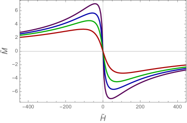
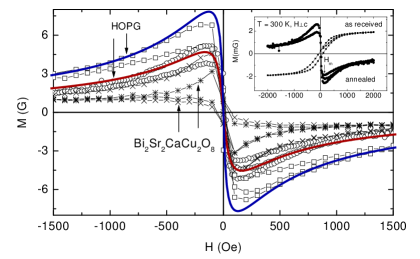
Figure 1: (a) The external magnetic field dependences of the magnetization at $T=0.8$(purple), $T=1$(blue), $T=1.2$(green) and $T=1.5$(red) with $q_{\chi}=10$, $\beta=2.2$, $\mu=0$. (b) Theory curve compared with experimental data of annealed highly oriented pyrolytic graphite(HOPG) sample for $T=150K$(rectangle) and $T=300K$(circle) in [33]. For comparison, the blue and red curves obtained by our formula (14) are added. The red one is for $T=1$, $\beta=2$ and the blue one is for $T=0.8$, $\beta=2.2$. $q_{\chi}=10$ and $\mu=0$ for both cases.

We want to analyse the magnetisation as a function of the magnetic field with the other parameters fixed. Notice that, at fix temperature, $r_{0}$ has to be computed from (7). In Figure 1 (a), we draw the magnetic field dependence of the magnetization at different temperatures for $\mu=0$, $q_{\chi}=10$, and $\beta=2$. The magnetization seems to be saturated for large magnetic field and the magnetic susceptibility is decreasing function of temperature. Our results are very similar to the graphite data in Figure 1 (b) [33]. Here, in addition to experimental data, we added the blue and red curves using our formula (14) for comparison, where the red one is for $T=1$, $\beta=2$ and the blue one is for $T=0.8$, $\beta=2.2$. $q_{\chi}=10$ and $\mu=0$ for both cases.

DC transport coefficients: Recently, a systematic way to compute the DC transport coefficients has been developed in [11, 12, 36] by which we can compute the longitudinal and transverse electric and thermoelectric conductivities. Here we write only result.

$$\begin{split}\sigma_{xx}&=\frac{({\cal F}-H^{2})({\cal F}+{\cal G}^{2})}{({\cal F}^{2}+H^{2}{\cal G}^{2})}\,,\cr\sigma_{xy}&=\frac{H{\cal G}(2{\cal F}+{\cal G}^{2}-H^{2})+\theta({\cal F}^{2}+H^{2}{\cal G}^{2})}{({\cal F}^{2}+H^{2}{\cal G}^{2})}\,,\cr\alpha_{xx}&=\frac{s\,{\cal G}({\cal F}-H^{2})}{{\cal F}^{2}+H^{2}{\cal G}^{2}}\,,\qquad\alpha_{xy}=\frac{s\,H({\cal F}+{\cal G}^{2})}{{\cal F}^{2}+H^{2}{\cal G}^{2}}\,,\end{split}$$ (16)

where

$$\begin{split}{\cal F}&=r_{0}^{2}\beta^{2}+H^{2}\left(1+\theta^{2}\right)-\theta qH\,,\cr{\cal G}&=q-\theta H,\qquad s=4\pi r_{0}^{2}\,.\end{split}$$ (17)

We gave some details at the end. We check two limits: i) for $\beta=0$, the DC conductivities (16) become $\sigma_{xx}=0$, $\sigma_{xy}=q/H$, $\alpha_{xx}=0$ and $\alpha_{xy}=s/H$, which agrees with [37]; ii) for $q_{\chi}=0$ (16) reproduces the result obtained in [12, 36].

At finite $\beta$ and finite $q_{\chi}$ but with $H=0$ the electric conductivities reduce to :

$$\sigma_{xx}=1+\frac{\mu^{2}}{\beta^{2}}\,,\qquad\sigma_{xy}=\theta=\frac{3M_{0}}{q}.$$ (18)

Notice that $\sigma_{xx}$ is a known result [32], but, interestingly, $\sigma_{xy}$ is non zero even when $H=0$. This phenomena is related to anomalous Hall effect, which will be discussed next. It is the result of the axion coupling we introduced, which gives a ferromagnetism with the magnetization $M_{0}$ (15).

Anomalous Hall effect: In ferromagnetic conductor, the Hall effect is about 10 times bigger than in non-magnetic material. This stronger Hall effect in ferromagnetic conductor is known as the anomalous Hall (AH) effect [38]. The precise mechanism for AH effect has a century-long history of debates [38]. Three mechanisms have been suggested : i) intrinsic one due to anomalous velocity, ii) side jump, iii) skew scattering. Mechanism i) was suggested in 1950’s by Karpulus and Luttinger. In modern days, the anomalous velocity is understood by the Berry phase (${\bf v}_{a}=\frac{e}{\hbar}{\bf E\times b}_{\rm Berry}$). Side jump mechanism is suggested by Berger in ref. [39] where he showed that the electron velocity is deflected in opposite directions by the opposite electric fields experienced upon approaching and leaving an impurity. The skew scattering was suggested by Smit in [40, 41] where he noticed that asymmetric scattering from impurities is caused by the spin-orbit interaction. The fundamental interaction underlying all these three is the spin-orbit interaction.

It has been known that there is a power law relationship between the anomalous part($R_{S}$) of the Hall resistivity($\rho_{yx}$) and the longitudinal resistivity($\rho_{xx}$):

$$R_{s}\sim\rho_{xx}^{\alpha}\,,$$ (19)

with the anomalous Hall coefficient, $R_{S}$, defined by the relation

$$\rho_{yx}=R_{H}H+R_{S}M,$$ (20)

where $R_{H}$ is the usual Hall coefficient. The power $\alpha$ had been computed for three scenarios to give $\alpha=2$ for i), ii) and $\alpha=1$ for iii).

From (14) and (18) our model describes a ferromagnetic conductor, therefore it will be interesting to study AH effect. The resistivity matrix($\rho$) can be computed by inverting the conductivity matrix($\sigma$) in (16) i.e. ${\cal\rho}={\cal\sigma}^{-1}$. $R_{S}$ is identified by $\rho_{yx}$ at $H=0$:

$$\rho_{yx}\Big{|}_{H=0}=\frac{\theta}{\theta^{2}+(1+\mu^{2}/\beta^{2})^{2}}=R_{S}M_{0}.$$ (21)

Since $M_{0}=\frac{1}{3}q\theta$, anomalous Hall coefficient is given by

$$R_{S}=\frac{3}{r_{0}\mu}\frac{1}{\theta^{2}+(1+\mu^{2}/\beta^{2})^{2}}.$$ (22)

The longitudinal resistivity at $H=0$ reads

$$\rho_{xx}=\frac{1+\mu^{2}/\beta^{2}}{\theta^{2}+(1+\mu^{2}/\beta^{2})^{2}}\,.$$ (23)

The scaling behaviours can be read easily for two limits:

$$R_{S}\sim\rho_{xx}^{2},\quad\hbox{or}\quad R_{S}\sim\rho_{xx},$$ (24)

depending on $\beta/\mu\ll 1$ or $\beta/\mu\gg 1$. The same scaling relations hold for $\theta\ll 1$ or $\theta\gg 1$.

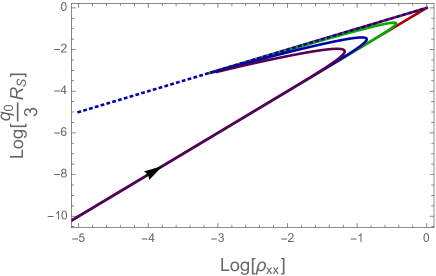
Figure 2: Relation between $\rho_{xx}$ and $\frac{q_{0}}{3}R_{s}$($q_{0}\equiv\mu r_{0}$) at fixed $q_{\chi}=1$ with $\mu/T=0.1$(red), $2$(green), $5$(blue) and $10$(purple) in log-log plot. The arrow represents the direction of increasing $\beta/\mu$. $R_{S}\sim\rho_{xx}^{2}$ in small $\beta/\mu$ and $R_{S}\sim\rho_{xx}$ in large $\beta/\mu$ regime.

For general value of $\beta/\mu$, the scaling behaviour is shown in Figure 2 as the slope. In the figure, the arrow represents the directions of increasing disorder parameter $\beta$, and $\mu/T=0.1$(red), $2$(green), $5$(blue) and $10$(purple). Notice the transition from $\alpha=2$ to $\alpha=1$ is sharper for larger temperature. Notice also that $\alpha=2$ for small $\beta/\mu$ whatever is the spin-orbit interaction strength $\theta$.

In ref. [35], material with $\beta/\mu\ll 1$ was identified as a coherent metal of which optical conductivity has a well defined Drude peak as if it had quasi particles. For $\beta/\mu\gg 1$, the system behaves as an incoherent metal without a Drude peak. Interestingly, such electrically classified coherent/incoherent metal also shows AH property with the characteristic power $\alpha=2,1$. This is consistent with the interpretation of $\beta$ as impurity density since large $\beta$ would have much extrinsic disorder effects. Notice that we have two scaling regimes in one model with interpolating parameters given by the disorder parameter $\beta$ or spin-orbit coupling strength $\theta$, while in conventional method different scalings are associated with different mechanisms. The fact that all three mechanisms are originated from spin-orbit interaction is reflected to our result which is a consequence of adding just one interaction term representing spin-orbit coupling.

Method: DC conductivites from black hole horizon
Here we explain how to obtain the DC conductivities (16). The action with counter terms are given by

$$\begin{split}2\kappa^{2}S=&\int_{\mathcal{M}}d^{4}x\sqrt{-g}\left\{R+\frac{6}{L^{2}}-\frac{1}{4}F^{2}-\sum_{I=1,2}\frac{1}{2}(\partial\chi_{I})^{2}\right\}-\frac{1}{16}\int_{\mathcal{M}}q_{\chi}{\left(\partial\chi_{I}\right)^{2}}F\wedge F+S_{c}\,,\cr&S_{c}=-\int_{\partial\mathcal{M}}d^{3}x\sqrt{-\gamma}\left(2K+\frac{4}{L}+R[\gamma]-\sum_{I=1,2}\frac{L}{2}\nabla\chi_{I}\cdot\nabla\chi_{I}\right)\,.\end{split}$$ (25)

The equations of motion are

$$\begin{split}&\nabla^{2}\chi_{I}+\frac{q_{\chi}}{8}\nabla_{M}\left(\frac{1}{\sqrt{-g}}\epsilon^{PQRS}F_{PQ}F_{RS}\nabla^{M}\chi_{I}\right)=0\,,\cr&\nabla_{M}F^{MN}+\frac{q_{\chi}}{4}\nabla_{M}\left((\partial\chi_{I})^{2}\frac{1}{\sqrt{-g}}\epsilon^{MNPQ}F_{PQ}\right)=0\,,\cr&R_{MN}-\frac{1}{2}g_{MN}\left(R+6-\frac{1}{4}F^{2}-\frac{1}{2}(\partial\chi_{I})^{2}\right)-\frac{1}{2}F_{MP}{F_{N}}^{P}-\frac{1}{2}\partial_{M}\chi_{I}\partial_{N}\chi_{I}\,,\cr&\qquad\qquad-\frac{q_{\chi}}{16}\partial_{M}\chi_{I}\partial_{N}\chi_{I}\frac{1}{\sqrt{-g}}\epsilon^{PQRS}F_{PQ}F_{RS}=0\,,\end{split}$$ (26)

where $\epsilon^{0123}=\epsilon^{txyr}=1$.

Once we get a background solution of these equations, we can compute the DC transport coefficients from the black hole horizon data. Let us start by defining a useful quantity:

$${\mathcal{F}}^{MN}\equiv\sqrt{-g}F^{MN}+\,\frac{q_{\chi}}{4}\left(\partial\chi\right)^{2}\epsilon^{MNPQ}F_{PQ}~{}~{}.$$ (27)

Then the Maxwell equation and the boundary current can be written as

$$\partial_{M}{\mathcal{F}}^{MN}=0~{}~{},~{}~{}J_{tot}^{\mu}=\lim_{r\to\infty}{\mathcal{F}}^{\mu r}\,.$$ (28)

If we assume all fields depend on $t$ and $r$, one can obtain another expression for the total boundary current using the Maxwell equation.

$$J_{tot}^{\mu}=\lim_{r\to r_{0}}{\mathcal{F}}^{\mu r}+\int_{r_{0}}^{\infty}dr\partial_{t}{\mathcal{F}}^{t\mu}~{}~{}.$$ (29)

Now we want to consider fluctuations corresponding to the boundary DC electric field $E_{i}$ and the DC temperature gradient $\zeta_{i}=\frac{\nabla_{i}T}{T}$. Following [11], we may consider fluctuations around the background as follows:

$$\begin{split}\delta A_{i}&=-\left(E_{i}-\zeta_{i}a(r)\right)\,t+\delta a_{i}(r)\,,\cr\delta g_{ti}&=-U(r)\,\zeta_{i}\,t+r^{2}\delta h_{ti}\,,\cr\delta g_{ri}&=r^{2}\delta h_{ri}\,,\cr\delta\chi_{i}&=\delta\chi_{i}(r)~{}~{}\,.\end{split}$$ (30)

In the linear level the time dependent part of the equations of motion drops out by the above choice of fluctuations. Thus these fluctuations are stable static fluctuations to the DC sources, $(E_{i},\zeta_{i})$.

To be a physical fluctuation in the black hole background, the fluctuation should satisfy the in-falling boundary condition as it approaches the horizon. This condition can be described in terms of the Eddington-Finkelstein coordinates $v=t+\frac{1}{4\pi T}\ln\left(r-r_{0}\right)$, and the in-falling fluctuation should depend on $v$ near horizon. Therefore, the regularity at the horizon implies

$$\begin{split}\delta h_{ti}&\sim-\frac{\zeta_{i}}{4\pi T}\log\left(r-r_{0}\right)\frac{U(r)}{r^{2}}+h_{ti}^{(0)}+{\cal O}((r-r_{0}))\,,\cr\delta h_{ri}&\sim\frac{\mathbb{H}_{ri}}{r^{2}U(r)}+h_{ri}^{(0)}+{\cal O}((r-r_{0}))\,,\cr\delta a_{i}&\sim-\frac{E_{i}-\zeta_{i}a(r)}{4\pi T}\log(r-r_{0})+a_{i}^{(0)}+{\cal O}((r-r_{0}))\,,\cr\delta\chi_{i}&\sim\delta\chi_{i}^{(0)}+{\cal O}((r-r_{0}))\,.\end{split}$$ (31)

By expanding $(r,i)$ component and $(t,i)$ component of the Einstein equations, it turns out that $\mathbb{H}_{ri}=r_{0}^{2}h_{ti}^{(0)}$ and $h_{ti}^{(0)}$ can be determined.

Now we are ready to consider the total current (29) in the linear level. The current can be calculated by plugging (4) and the fluctuation (30). Firstly, the second part is

$$\int_{r_{0}}^{\infty}dr\partial_{t}{\mathcal{F}}^{ti}=\frac{\epsilon_{ij}}{r_{0}}\left(-{H}+\frac{1}{3}\theta q-\frac{1}{5}\theta^{2}H\right)\zeta_{j}\,.$$ (32)

This is nothing but the magnetization current $J^{i}_{mag}=-\epsilon^{ij}\tilde{M}\frac{\partial_{j}T}{T}$ [42] which should be subtracted. Thus the relevant part of the current is the first term, which can be written in terms of the horizon data:

$$J^{\mu}=\lim_{r\to r_{0}}{\mathcal{F}}^{\mu r}=E_{i}-\left(q-\theta H\right)h_{ti}^{(0)}-\frac{H}{r_{0}^{2}}\epsilon_{ij}\mathbb{H}_{rj}+\epsilon_{ij}\theta E_{j}~{}~{}.$$ (33)

Finally, the expressions $h^{(0)}_{ti}$ and $\mathbb{H}_{ri}$ obtained from the Einstein equation give us the electric conductivities and the thermoelectric coefficients (16) using formula $\sigma_{ij}=\frac{\partial J^{i}}{\partial E_{j}}$ and $\alpha_{ij}=\frac{1}{T}\frac{\partial J^{i}}{\partial\zeta_{j}}$.

Summary and Discussion: We view the holographic principle as a set of axioms to calculate strongly interacting systems. For reader’s convenience we first list them below [9].

1. For a strongly interacting system with conformal symmetry at UV, there is a dual gravity with asymptotic AdS boundary. Non AdS geometry may be regarded as an IR part of an asymptotic AdS geometry.

2. To calculate the correlation function of an operator ${\cal O}_{\Delta}$ with dimension $\Delta$ and spin $p$, we introduce a source field $\phi_{0}(x)$ with spin $p$ and dimension $\Delta$. Extend $\phi_{0}(x)$ into one higher dimensional space $\phi(x,r)$ such that $\phi(x,r=\infty)\sim\phi_{0}(x)/r^{d-2p-\Delta}$. Identify the generating function of conformal field theory $Z[\phi_{0}]$ with that of gravitational system $exp(-S[\phi_{0}])$.

3. For a global symmetry at the bulk, we have a local gauge symmetry at the boundary.

4. For Euclidean Green functions, Dirichlet boundary value at infinity is enough. For causal green function, assign the boundary condition (BC) at the IR region in addition to the Dirichlet BC at the infinity.

5. Temperature and chemical potential are provided by regularity of metric, gauge fields at the horizon or its replacing IR geometry.

6. Characterise the system by lifting the least irrelevant interactions at the boundary to the bulk. For strongly correlated electron system, the electron-electron interaction is counted by the gravity, but electron-lattice interactions should be taken into account explicitly. The gauge field dual to the conserved $U(1)$ current can have interaction terms to take care of electron-lattice interactions.

The last item is what we added in this paper. In this paper, we considered the magneto-electric phenomena induced by the spin-orbit coupling interaction as an example of dimensional lifting in holographic theory. When electron spins are correlated, adding charge carrier changes the magnetic property as well as the charge transport. In effective field theory approach, such electric-magnetic effect can be implied by adding the Chern-Simons term $\sim A\wedge F$ in 2+1 dimension. It act as a crossing source of electricity and magnetism. With such a term, the system can pick up a magnetic source when we provide electric charge and vice versa.

We work at finite temperature, chemical potential, and magnetic fields. The metric, gauge and axion fields ($g_{\mu\nu},A_{\mu},\chi_{I}$) are playing the role of coupled order parameters. We have found the exact and analytic solution of such a complicated coupled system with a non-trivial interaction, which made it possible to get an explicit and analytic DC conductivity formulas.

Our results on the Hall resistivity shows a non-linear diamagnetic response is similar to that of graphite system and also to high $T_{c}$ superconductor $\rm Bi_{2}Sr_{2}CaCu_{2}O_{8}$. Also we have shown that the anomalous Hall coefficients in our model interpolate between the linear and quadratic regime on the resistivity dependence as a function of disorder parameter and spin-orbit interaction coupling. It is particularly interesting to see that electrical coherent/incoherent metal has magnetic behaviour with quadratic/linear resistivity dependence. Experimentally diverse materials were studied. Some shows $\alpha$ near 2 and the other 1, sometimes old and new data crashes. So, Detailed data mining is postponed to future investigation.

Our model does not include paramagnetic behaviour because we integrated out fermion and therefore spin degrees of freedom is not included explicitly. Also we could have chosen the scalar field $\chi$ itself instead of its kinetic term as a scalar partner of $F\wedge F$ term. We will report on these issues elsewhere.

References

- [1] Juan Martin Maldacena. The Large N limit of superconformal field theories and supergravity. Int.J.Theor.Phys., 38:1113–1133, 1999.
- [2] Edward Witten. Anti-de Sitter space and holography. Adv. Theor. Math. Phys., 2:253–291, 1998.
- [3] S. S. Gubser, Igor R. Klebanov, and Alexander M. Polyakov. Gauge theory correlators from noncritical string theory. Phys. Lett., B428:105–114, 1998.
- [4] Steven S. Gubser. Breaking an Abelian gauge symmetry near a black hole horizon. Phys.Rev., D78:065034, 2008.
- [5] Sean A. Hartnoll, Christopher P. Herzog, and Gary T. Horowitz. Holographic Superconductors. JHEP, 12:015, 2008.
- [6] Frederik Denef and Sean A Hartnoll. Landscape of superconducting membranes. Physical Review D, 79(12):126008, 2009.
- [7] Aristomenis Donos and Sean A. Hartnoll. Interaction-driven localization in holography. Nature Phys., 9:649–655, 2013.
- [8] Thomas Faulkner and Joseph Polchinski. Semi-Holographic Fermi Liquids. JHEP, 06:012, 2011.
- [9] Sean A. Hartnoll. Horizons, holography and condensed matter. 2011.
- [10] Aristomenis Donos and Jerome P. Gauntlett. Novel metals and insulators from holography. JHEP, 06:007, 2014.
- [11] Aristomenis Donos and Jerome P. Gauntlett. Thermoelectric DC conductivities from black hole horizons. JHEP, 1411:081, 2014.
- [12] Keun-Young Kim, Kyung Kiu Kim, Yunseok Seo, and Sang-Jin Sin. Thermoelectric Conductivities at Finite Magnetic Field and the Nernst Effect. 2015.
- [13] Xian-Hui Ge, Yi Ling, Chao Niu, and Sang-Jin Sin. Thermoelectric conductivities, shear viscosity, and stability in an anisotropic linear axion model. Phys. Rev., D92(10):106005, 2015.
- [14] M Zahid Hasan and Charles L Kane. Colloquium: topological insulators. Reviews of Modern Physics, 82(4):3045, 2010.
- [15] Xiao-Liang Qi and Shou-Cheng Zhang. Topological insulators and superconductors. Reviews of Modern Physics, 83(4):1057, 2011.
- [16] Liang Fu and Charles L Kane. Topological insulators with inversion symmetry. Physical Review B, 76(4):045302, 2007.
- [17] Haijun Zhang, Chao-Xing Liu, Xiao-Liang Qi, Xi Dai, Zhong Fang, and Shou-Cheng Zhang. Topological insulators in bi2se3, bi2te3 and sb2te3 with a single dirac cone on the surface. Nature physics, 5(6):438–442, 2009.
- [18] Karl Landsteiner, Yan Liu, and Ya-Wen Sun. A quantum phase transition between a topological and a trivial semi-metal in holography. 2015.
- [19] Rundong Li, Jing Wang, Xiao-Liang Qi, and Shou-Cheng Zhang. Dynamical axion field in topological magnetic insulators. Nature Physics, 6(4):284–288, 2010.
- [20] Heon-Jung Kim, Ki-Seok Kim, J-F Wang, M Sasaki, N Satoh, A Ohnishi, M Kitaura, M Yang, and L Li. Dirac versus weyl fermions in topological insulators: Adler-bell-jackiw anomaly in transport phenomena. Physical review letters, 111(24):246603, 2013.
- [21] Yeong-Chuan Kao and Mahiko Suzuki. Radiatively induced topological mass terms in (2+ 1)-dimensional gauge theories. Physical Review D, 31(8):2137, 1985.
- [22] Marc D Bernstein and Taejin Lee. Radiative corrections to the topological mass in (2+ 1)-dimensional electrodynamics. Physical Review D, 32(4):1020, 1985.
- [23] Stefan Hohenegger and Ingo Kirsch. A note on the holography of chern-simons matter theories with flavour. Journal of High Energy Physics, 2009(04):129, 2009.
- [24] Mitsutoshi Fujita, Wei Li, Shinsei Ryu, and Tadashi Takayanagi. Fractional quantum hall effect via holography: Chern-simons, edge states and hierarchy. Journal of High Energy Physics, 2009(06):066, 2009.
- [25] Yoshinori Matsuo, Sang-Jin Sin, Shingo Takeuchi, and Takuya Tsukioka. Chern-simons term in holographic hydrodynamics of charged ads black hole. Journal of High Energy Physics, 2010(4):1–18, 2010.
- [26] Aristomenis Donos, Jerome P Gauntlett, and Christiana Pantelidou. Spatially modulated instabilities of magnetic black branes. Journal of High Energy Physics, 2012(1):1–18, 2012.
- [27] Shin Nakamura, Hirosi Ooguri, and Chang-Soon Park. Gravity dual of spatially modulated phase. Physical Review D, 81(4):044018, 2010.
- [28] Hirosi Ooguri and Chang-Soon Park. Holographic endpoint of spatially modulated phase transition. Physical Review D, 82(12):126001, 2010.
- [29] Sophia K Domokos and Jeffrey A Harvey. Baryon-number-induced chern-simons couplings of vector and axial-vector mesons in holographic qcd. Physical review letters, 99(14), 2007.
- [30] Aristomenis Donos and Jerome P Gauntlett. Holographic striped phases. Journal of High Energy Physics, 2011(8):1–17, 2011.
- [31] Oren Bergman, Niko Jokela, Gilad Lifschytz, and Matthew Lippert. Striped instability of a holographic fermi-like liquid. Journal of High Energy Physics, 2011(10):1–14, 2011.
- [32] Tomas Andrade and Benjamin Withers. A simple holographic model of momentum relaxation. JHEP, 1405:101, 2014.
- [33] Y. Kopelevich, P. Esquinazi, J. H. S. Torres, and S. Moehlecke. Ferromagnetic- and superconducting-like behavior of graphite. J. Low Temp. Phys., 119:691, 2000.
- [34] LD Landau, LP Pitaevskii, and EM Lifshitz. Electrodynamics of continuous media: Volume 8 (course of theoretical physics). 1984.
- [35] Keun-Young Kim, Kyung Kiu Kim, Yunseok Seo, and Sang-Jin Sin. Coherent/incoherent metal transition in a holographic model. JHEP, 1412:170, 2014.
- [36] Mike Blake, Aristomenis Donos, and Nakarin Lohitsiri. Magnetothermoelectric Response from Holography. 2015.
- [37] Sean A. Hartnoll and Pavel Kovtun. Hall conductivity from dyonic black holes. Phys. Rev., D76:066001, 2007.
- [38] Naoto Nagaosa. Anomalous hall effect. Reviews of Modern Physics, 82(2):1539–1592, 2010.
- [39] L Berger. Side-jump mechanism for the hall effect of ferromagnets. Physical Review B, 2(11):4559, 1970.
- [40] J Smit. The spontaneous hall effect in ferromagnetics i. Physica, 21(6):877–887, 1955.
- [41] Jan Smit. The spontaneous hall effect in ferromagnetics ii. Physica, 24(1):39–51, 1958.
- [42] N. R. Cooper. Thermoelectric response of an interacting two-dimensional electron gas in a quantizing magnetic field. Physical Review B, 55(4):2344–2359, 1997.