Abstract

In this article we formally investigate the impact of twisted space-time on black-body radiation phenomena, i.e. we derive the $\theta$-deformed Planck distribution function as well as we perform its numerical integration to the $\theta$-deformed total radiation energy. In such a way we indicate that the space-time noncommutativity very strongly damps the black-body radiation process. Besides we provide for small parameter $\theta$ the twisted counterparts of Rayleigh-Jeans and Wien distributions respectively.

1 Introduction

The suggestion to use noncommutative coordinates goes back to Heisenberg and was firstly formalized by Snyder in [1]. Recently, there were also found formal arguments based mainly on Quantum Gravity [2], [3] and String Theory models [4], [5], indicating that space-time at Planck scale should be noncommutative, i.e., it should have a quantum nature. Consequently, there are a number of papers dealing with noncommutative classical and quantum mechanics (see e.g. [6]-[9]) as well as with field theoretical models (see e.g. [10]-[12]) in which the quantum space-time is employed.

It is well-known that a proper modification of the Poincare and Galilei Hopf algebras can be realized in the framework of Quantum Groups [13], [14]. Hence, in accordance with the Hopf-algebraic classification of all deformations of relativistic and nonrelativistic symmetries (see [15], [16]), one can distinguish three types of quantum spaces [15], [16] (for details see also [17]):

1) Canonical ($\theta^{\mu\nu}$-deformed) type of quantum space [18]-[20]

$$[\;{x}_{\mu},{x}_{\nu}\;]=i\theta_{\mu\nu}\;,$$ (1)

2) Lie-algebraic modification of classical space-time [20]-[23]

$$[\;{x}_{\mu},{x}_{\nu}\;]=i\theta_{\mu\nu}^{\rho}{x}_{\rho}\;,$$ (2)

and

3) Quadratic deformation of Minkowski and Galilei spaces [20], [23]-[25]

$$[\;{x}_{\mu},{x}_{\nu}\;]=i\theta_{\mu\nu}^{\rho\tau}{x}_{\rho}{x}_{\tau}\;,$$ (3)

with coefficients $\theta_{\mu\nu}$, $\theta_{\mu\nu}^{\rho}$ and $\theta_{\mu\nu}^{\rho\tau}$ being constants.

Moreover, it has been demonstrated in [17], that in the case of the so-called N-enlarged Newton-Hooke Hopf algebras $\,{\mathcal{U}}^{(N)}_{0}({NH}_{\pm})$ the twist deformation provides the new space-time noncommutativity of the form,

$${\bf 4)}\;\;\;\;\;\;\;\;\;[\;t,{x}_{i}\;]=0\;\;\;,\;\;\;[\;{x}_{i},{x}_{j}\;]=if_{\pm}\left(\frac{t}{\tau}\right)\theta_{ij}(x)\;,$$ (4)

with time-dependent functions

$$f_{+}\left(\frac{t}{\tau}\right)=f\left(\sinh\left(\frac{t}{\tau}\right),\cosh\left(\frac{t}{\tau}\right)\right)\;\;\;,\;\;\;f_{-}\left(\frac{t}{\tau}\right)=f\left(\sin\left(\frac{t}{\tau}\right),\cos\left(\frac{t}{\tau}\right)\right)\;,$$

$\theta_{ij}(x)\sim\theta_{ij}={\rm const}$ or $\theta_{ij}(x)\sim\theta_{ij}^{k}x_{k}$ and $\tau$ denoting the time scale parameter - the cosmological constant. Besides, it should be noted that the mentioned above quantum spaces 1), 2) and 3) can be obtained by the proper contraction limit of the commutation relations 4).

Recently, there has been discussed the impact of different kinds of quantum spaces on the dynamical structure of physical systems (see e.g. [6]-[11] and [26]-[38]). Particulary, it has been demonstrated, that in the case of a classical oscillator model [29] as well as in the case of a nonrelativistic particle moving in constant external field force $\vec{F}$ [30], there are generated by space-time noncommutativity additional force terms. Such a type of investigation has been performed for quantum oscillator model as well [29], i.e., it was demonstrated that the quantum space in nontrivial way affects the spectrum of the energy operator. Besides, in the paper [31] there has been considered a model of a particle moving on the $\kappa$-Galilei space-time in the presence of gravitational field force. It has been demonstrated, that in such a case there is produced a force term, which can be identified with the so-called Pioneer anomaly [33], and the value of the deformation parameter $\kappa$ can be fixed by a comparison of obtained result with observational data. Moreover, the quite interesting results have been obtained in the series of papers [34]-[37] concerning the Hall effect for canonically deformed space-time (1). Particularly, there has been found the $\theta$-dependent (Landau) energy spectrum of an electron moving in uniform magnetic as well as in uniform electric field. Such results have been generalized to the case of the twisted N-enlarged Newton-Hooke Hopf algebra in paper [39] and [40]. Finally, it should be mentioned that similar investigation has been performed in the context of black-body radiation process as well. For example, it has been demonstrated with use of noncommutative electromagnetic field theory that black-body radiation for quantum space becomes anisotropic. A direct implication of such a result on Cosmic Microwave Background map has been argued in papers [41] and [42].

In this article we also investigate the impact of twisted space-time on black-body radiation phenomena. However we assume that a single mode of photon field oscillates with frequency predicted by new, first-quantized and canonically noncommutative oscillator model. Precisely we derive the $\theta$-deformed Planck distribution function as well as we perform its numerical integration to the $\theta$-deformed total radiation energy. In such a way we indicate that the space-time noncommutativity very strongly damps the black-body radiation process. Besides we provide for small parameter $\theta$ the twisted counterparts of Rayleigh-Jeans and Wien distributions respectively.

The paper is organized as follows. In Sect. 2 we recall basic facts concerning the most wide class of twisted (N-enlarged Newton-Hooke) space-times [17] which includes the canonically deformed one as well. The third section is devoted to the calculation of isotropic energy spectrum for the oscillator model defined on such quantum spaces. In section four the Planck distribution function is provided and its numerical integration to the $\theta$-deformed total radiation energy is performed. The final remarks are presented in the last section.

2 Twisted N-enlarged Newton-Hooke space-times

In this section we recall the basic facts associated with the twisted N-enlarged Newton-Hooke Hopf algebra $\;{\cal U}^{(N)}_{\alpha}(NH_{\pm})$ and with the corresponding quantum space-times [17]. Firstly, it should be noted that in accordance with Drinfeld twist procedure, the algebraic sector of twisted Hopf structure $\;{\cal U}^{(N)}_{\alpha}(NH_{\pm})$ remains undeformed, i.e., it takes the form

$$\left[\,M_{ij},M_{kl}\,\right]=i\left(\delta_{il}\,M_{jk}-\delta_{jl}\,M_{ik}+\delta_{jk}M_{il}-\delta_{ik}M_{jl}\right)\;\;\;,\;\;\;\left[\,H,M_{ij}\,\right]=0\;,$$ (5)

(7)

$$\left[\,M_{ij},G_{k}^{(n)}\,\right]=i\left(\delta_{jk}\,G_{i}^{(n)}-\delta_{ik}\,G_{j}^{(n)}\right)\;\;\;,\;\;\;\left[\,G_{i}^{(n)},G_{j}^{(m)}\,\right]=0\;,$$

(9)

$$\left[\,G_{i}^{(k)},H\,\right]=-ikG_{i}^{(k-1)}\;\;\;,\;\;\;\left[\,H,G_{i}^{(0)}\,\right]=\pm\frac{i}{\tau}G_{i}^{(1)}\;\;\;;\;\;\;k>1\;,$$

where $\tau$, $M_{ij}$, $H$, $G_{i}^{(0)}(=P_{i})$, $G_{i}^{(1)}(=K_{i})$ and $G_{i}^{(n)}(n>1)$ can be identified with cosmological time parameter, rotation, time translation, momentum, boost and accelerations operators respectively. Besides, the coproducts and antipodes of considered algebra are given by

$$\Delta_{\alpha}(a)=\mathcal{F}_{\alpha}\circ\,\Delta_{0}(a)\,\circ\mathcal{F}_{\alpha}^{-1}\;\;\;,\;\;\;S_{\alpha}(a)=u_{\alpha}\,S_{0}(a)\,u^{-1}_{\alpha}\;,$$ (10)

with $u_{\alpha}=\sum f_{(1)}S_{0}(f_{(2)})$ (we use the Sweedler’s notation $\mathcal{F}_{\alpha}=\sum f_{(1)}\otimes f_{(2)}$) and with the twist factor $\mathcal{F}_{\alpha}\in{\cal U}^{(N)}_{\alpha}(NH_{\pm})\otimes{\cal U}^{(N)}_{\alpha}(NH_{\pm})$ satisfying the classical cocycle condition

$${\mathcal{F}}_{{\alpha}12}\cdot(\Delta_{0}\otimes 1)~{}{\cal F}_{\alpha}={\mathcal{F}}_{{\alpha}23}\cdot(1\otimes\Delta_{0})~{}{\mathcal{F}}_{{\alpha}}\;,$$ (11)

and the normalization condition

$$(\epsilon\otimes 1)~{}{\cal F}_{{\alpha}}=(1\otimes\epsilon)~{}{\cal F}_{{\alpha}}=1\;,$$ (12)

such that ${\cal F}_{{\alpha}12}={\cal F}_{{\alpha}}\otimes 1$ and ${\cal F}_{{\alpha}23}=1\otimes{\cal F}_{{\alpha}}$.

The corresponding quantum space-times are defined as the representation spaces (Hopf modules) for the N-enlarged Newton-Hooke Hopf algebra  ${\cal U}_{\alpha}^{(N)}(NH_{\pm})$. Generally, they are equipped with two the spatial directions commuting to classical time, i.e. they take the form

$$[\;t,\hat{x}_{i}\;]=[\;\hat{x}_{1},\hat{x}_{3}\;]=[\;\hat{x}_{2},\hat{x}_{3}\;]=0\;\;\;,\;\;\;[\;\hat{x}_{1},\hat{x}_{2}\;]=if({t})\;\;;\;\;i=1,2,3\;.$$ (13)

However, it should be noted that this type of noncommutativity has been constructed explicitly only in the case of the 6-enlarged Newton-Hooke Hopf algebra, with [17]

$$f({t}) = f_{\kappa_{1}}({t})=f_{\pm,\kappa_{1}}\left(\frac{t}{\tau}\right)=\kappa_{1}\,C_{\pm}^{2}\left(\frac{t}{\tau}\right)\;,$$

$$f({t}) = f_{\kappa_{2}}({t})=f_{\pm,\kappa_{2}}\left(\frac{t}{\tau}\right)=\kappa_{2}\tau\,C_{\pm}\left(\frac{t}{\tau}\right)S_{\pm}\left(\frac{t}{\tau}\right)\;,$$

$$~{}~{}~{}~{}~{}~{}~{}~{}~{}~{}~{}~{}~{}~{}~{}~{}~{}~{}~{}~{}~{}~{}~{}~{}~{}~{}~{}~{}~{}~{}~{}~{}~{}\cdot$$

$$~{}~{}~{}~{}~{}~{}~{}~{}~{}~{}~{}~{}~{}~{}~{}~{}~{}~{}~{}~{}~{}~{}~{}~{}~{}~{}~{}~{}~{}~{}~{}~{}~{}\cdot$$

$$~{}~{}~{}~{}~{}~{}~{}~{}~{}~{}~{}~{}~{}~{}~{}~{}~{}~{}~{}~{}~{}~{}~{}~{}~{}~{}~{}~{}~{}~{}~{}~{}~{}\cdot$$

$$f({t}) = f_{\kappa_{35}}\left(\frac{t}{\tau}\right)=86400\kappa_{35}\,\tau^{11}\left(\pm C_{\pm}\left(\frac{t}{\tau}\right)\mp\frac{1}{24}\left(\frac{t}{\tau}\right)^{4}-\frac{1}{2}\left(\frac{t}{\tau}\right)^{2}\mp 1\right)\,\times$$

$$~{}~{}~{}~{}~{}~{}~{}~{}~{}~{}~{}~{}~{}~{}~{}~{}\times~{}\;\left(S_{\pm}\left(\frac{t}{\tau}\right)\mp\frac{1}{6}\left(\frac{t}{\tau}\right)^{3}-\frac{t}{\tau}\right)\;,$$

$$f({t}) = f_{\kappa_{36}}\left(\frac{t}{\tau}\right)=518400\kappa_{36}\,\tau^{12}\left(\pm C_{\pm}\left(\frac{t}{\tau}\right)\mp\frac{1}{24}\left(\frac{t}{\tau}\right)^{4}-\frac{1}{2}\left(\frac{t}{\tau}\right)^{2}\mp 1\right)^{2}\;,$$

and

$$C_{+/-}\left(\frac{t}{\tau}\right)=\cosh/\cos\left(\frac{t}{\tau}\right)\;\;\;{\rm and}\;\;\;S_{+/-}\left(\frac{t}{\tau}\right)=\sinh/\sin\left(\frac{t}{\tau}\right)\;.$$

Moreover, one can easily check that when $\tau$ is approaching the infinity limit the above quantum spaces reproduce the canonical (1), Lie-algebraic (2) and quadratic (3) type of space-time noncommutativity, i.e., for $\tau\to\infty$ we get

$$f_{\kappa_{1}}({t}) = \kappa_{1}\;,$$

$$f_{\kappa_{2}}({t}) = \kappa_{2}\,t\;,$$

$$\cdot$$

$$\cdot$$

$$\cdot$$

$$f_{\kappa_{35}}({t}) = \kappa_{35}\,t^{11}\;,$$

$$f_{\kappa_{36}}({t}) = \kappa_{36}\,t^{12}\;.$$

Of course, for all deformation parameters $\kappa_{a}$ going to zero the above deformations disappear.

3 Quantum oscillator model for twisted N-enlarged Newton-Hooke space-time

Let us now turn to the oscillator model defined on quantum space-times (13)-(2). In first step of our construction, we extend the described in pervious section spaces to the whole algebra of momentum and position operators as follows

$$[\;\hat{x}_{1},\hat{x}_{2}\;]=2if_{\kappa_{a}}({t})\;\;\;,\;\;\;[\;\hat{p}_{1},\hat{p}_{2}\;]=2ig_{\kappa_{a}}({t})\;,$$ (16)

$$[\;\hat{x}_{i},\hat{p}_{j}\;]=i\hbar\delta_{ij}\left[1+f_{\kappa_{a}}({t})g_{\kappa_{a}}({t})/\hbar^{2}\right]\;,$$ (17)

with the arbitrary function $g_{\kappa_{a}}({t})$. One can check that relations (16), (17) satisfy the Jacobi identity and for deformation parameters $\kappa_{a}$ approaching zero become classical.
Next, by analogy to the commutative case, we define the Hamiltonian operator

$$\hat{H}=\frac{1}{2m}\left({\hat{{p}}_{1}^{2}}+{\hat{{p}}_{2}^{2}}\right)+\frac{1}{2}m\omega^{2}\left({\hat{{x}}_{1}^{2}}+{\hat{{x}}_{2}^{2}}\right)\;.$$ (18)

with $m$ and $\omega$ denoting the mass and frequency of a particle, respectively.
In order to analyze the above system, we represent the noncommutative operators $({\hat{x}}_{i},{\hat{p}}_{i})$ by the classical ones $({x}_{i},{p}_{i})$ as (see e.g. [27]-[29])

$${\hat{x}}_{1} = {x}_{1}-{f_{\kappa_{a}}(t)}p_{2}/\hbar\;,$$ (19)

$${\hat{x}}_{2} = {x}_{2}+{f_{\kappa_{a}}(t)}p_{1}/\hbar\;,$$ (20)

$${\hat{p}}_{1} = {p}_{1}+{g_{\kappa_{a}}(t)}x_{2}/\hbar\;,$$ (21)

$${\hat{p}}_{2} = {p}_{2}-{g_{\kappa_{a}}(t)}x_{1}/\hbar\;,$$ (22)

where

$$[\;x_{i},x_{j}\;]=0=[\;p_{i},p_{j}\;]\;\;\;,\;\;\;[\;x_{i},p_{j}\;]={i\hbar}\delta_{ij}\;.$$ (23)

Then, the Hamiltonian (18) takes the form

$$\hat{H}=\hat{H}(t)=\frac{1}{2M(t)}\left({{{p}}_{1}^{2}}+{{{p}}_{2}^{2}}\right)+\frac{1}{2}M(t)\Omega^{2}(t)\left({{{x}}_{1}^{2}}+{{{x}}_{2}^{2}}\right)-S(t)L\;,$$ (24)

with

$$L=x_{1}p_{2}-x_{2}p_{1}\;,$$ (25)

$$1/M(t)=1/m+m\omega^{2}f_{\kappa_{a}}^{2}(t)/\hbar^{2}\;,$$ (26)

$$\Omega(t)=\sqrt{\left(1/m+m\omega^{2}f_{\kappa_{a}}^{2}(t)/\hbar^{2}\right)\left(m\omega^{2}+g_{\kappa_{a}}^{2}(t)/(\hbar^{2}m)\right)}\;,$$ (27)

and

$$S(t)=m\omega^{2}f_{\kappa_{a}}(t)/\hbar+g_{\kappa_{a}}(t)/(\hbar m)\;.$$ (28)

In accordance with the scheme proposed in [29], we introduce a set of time-dependent creation $(a^{{\dagger}}_{A}(t))$ and annihilation $(a_{A}(t))$ operators

$$\hat{a}_{\pm}(t) = \frac{1}{2}\left[\frac{({p}_{2}\pm i{p}_{1})}{\sqrt{M(t)\Omega(t)\hbar}}-i\sqrt{M(t)\Omega(t)/\hbar}({x}_{2}\pm i{x}_{1})\right]\;,$$ (29)

satisfying the standard commutation relations

$$[\;\hat{a}_{A},\hat{a}_{B}\;]=0\;\;,\;\;[\;\hat{a}^{{\dagger}}_{A},\hat{a}^{{\dagger}}_{B}\;]=0\;\;,\;\;[\;\hat{a}_{A},\hat{a}^{{\dagger}}_{B}\;]=\delta_{AB}\;\;\;;\;\;A,B=\pm\;.$$ (30)

Then, it is easy to see that in terms of the objects (29) the Hamiltonian function (24) can be written as follows

$${\hat{H}}(t)=\hbar\Omega_{+}(t)\left[{\hat{N}}_{+}(t)+\frac{1}{2}\right]+\hbar\Omega_{-}(t)\left[{\hat{N}}_{-}(t)+\frac{1}{2}\right]\;,$$ (31)

with the coefficient $\Omega_{\pm}(t)$ and the particle number operators $\hat{N}_{\pm}(t)$ given by

$$\Omega_{\pm}(t) = \Omega(t)\mp S(t)\;,$$ (32)

$${\hat{N}}_{\pm}(t) = {\hat{a}}^{{\dagger}}_{\pm}(t){\hat{a}}_{\pm}(t)\;.$$ (33)

Besides, one can observe that the eigenvectors of Hamiltonian (31) can be written as

$$|n_{+},n_{-},t>=\frac{1}{\sqrt{n_{+}!}}\frac{1}{\sqrt{n_{-}!}}\left({\hat{a}}^{{\dagger}}_{+}(t)\right)^{n_{+}}\left({\hat{a}}^{{\dagger}}_{-}(t)\right)^{n_{-}}|0>\;,$$ (34)

while the corresponding eigenvalues take the form

$$E_{n_{+},n_{-}}(t)=\hbar\Omega_{+}(t)\left[n_{+}+\frac{1}{2}\right]+\hbar\Omega_{-}(t)\left[n_{-}+\frac{1}{2}\right]\;.$$ (35)

Let us now consider an interesting situation such that

$$S(t)=0\;.$$ (36)

One can check that it appears when functions $f_{\kappa_{a}}(t)$ and $g_{\kappa_{a}}(t)$ satisfy the following condition

$$f_{\kappa_{a}}(t)=-{g_{\kappa_{a}}(t)}/({\omega^{2}m^{2}})\;.$$ (37)

Then, we have

$$\Omega_{-}(t)=\Omega_{+}(t)=\Omega(t)=m\omega\left({1}/{m}+{m\omega^{2}}f_{\kappa_{a}}^{2}(t)/{\hbar^{2}}\right)\;,$$ (38)

and, consequently, the spectrum (35) provides the energy levels for two-dimensional isotropic oscillator model with the time-dependent frequency $\Omega(t)$

$$E_{n_{+},n_{-}}(t)=\hbar\Omega(t)\left[n_{+}+\frac{1}{2}\right]+\hbar\Omega(t)\left[n_{-}+\frac{1}{2}\right]\;.$$ (39)

Particularly, for canonical deformation $f_{\kappa_{1}}(t)=\kappa_{1}=\theta$ we get

$$E_{n_{+},n_{-},\theta}=\hbar\Omega_{\theta}\left[n_{+}+\frac{1}{2}\right]+\hbar\Omega_{\theta}\left[n_{-}+\frac{1}{2}\right]\;,$$ (40)

with constant frequency

$$\Omega_{\theta}=\Omega_{\theta}(\omega)=m\omega\left({1}/{m}+{m\omega^{2}}\theta^{2}/{\hbar^{2}}\right)\;,$$ (41)

such that $\lim_{\theta\to 0}\Omega_{\theta}=\omega$.

4 Black-body radiation for twisted space-time

In this section we derive the black-body radiation for $\theta$-deformed nonrelativistic space, i.e. due to the results of pervious section we take under consideration the following energies of a single mode of photon field

$$E_{n,\theta}(\omega)=\hbar\Omega_{\theta}(\omega)n\;\;\;;\;\;\;n=1,2,3,\;\ldots\;,$$ (42)

where factor $\Omega_{\theta}(\omega)$ is given just by (41). Consequently, in accordance with quantum theory [43] its average energy takes the form

$$\overline{E}_{\theta}(\omega)=\frac{\hbar\Omega_{\theta}(\omega)}{\exp\left(\frac{\hbar\Omega_{\theta}(\omega)}{kT}\right)-1}\;,$$ (43)

with Boltzman constant $k$ and temperature $T$. Besides, due to the fact that the number of state with frequency from $\omega$ to $\omega+d\omega$ per volume unit is [43], [44]

$$\rho(\omega)d\omega=\frac{8\pi\omega^{2}}{c^{3}}d\omega\;,$$ (44)

we get the following $\theta$-deformed Planck distribution function

$$f_{\theta}(\omega)=\frac{8\pi\hbar\omega^{2}}{c^{3}}\cdot\frac{\Omega_{\theta}(\omega)}{\exp\left(\frac{\hbar\Omega_{\theta}(\omega)}{kT}\right)-1}\;.$$ (45)

Of course, in $\theta$ approaching zero limit we reproduce from (45) well-known Planck formula

$$f(\omega)=\frac{8\pi\hbar}{c^{3}}\cdot\frac{\omega^{3}}{\exp\left(\frac{\hbar\omega}{kT}\right)-1}\;,$$ (46)

while for small values of deformation parameter, we have

$$f_{\theta}(\omega) = \frac{8\pi\hbar}{c^{3}}\cdot\frac{\omega^{3}}{\exp\left(\frac{\hbar\omega}{kT}\right)-1}\;+$$

$$- \frac{8\pi\hbar}{c^{3}}\cdot\frac{m^{2}\omega^{5}\left(\hbar\omega\exp\left(\frac{\hbar\omega}{kT}\right)-kT\left(\exp\left(\frac{\hbar\omega}{kT}\right)-1\right)\right)\theta^{2}}{\left(\exp\left(\frac{\hbar\omega}{kT}\right)-1\right)^{2}\hbar^{2}kT}\;+$$

$$+ {\cal O}(\theta^{3})\;.$$

Besides in accordance with (4) in high-temperature $(kT>>\hbar\omega)$ as well as in high-frequency $(\hbar\omega>>kT)$ limit, we obtain the $\theta$-deformed counterparts of Rayleigh-Jeans

$$f_{\theta}(\omega) = \frac{8\pi\omega^{2}\hbar^{2}kT}{c^{3}}-\frac{8\pi m^{2}\omega^{5}kT\theta^{2}}{c^{3}\hbar}+{\cal O}(\theta^{3})\;,$$ (48)

and Wien

$$f_{\theta}(\omega) = \frac{8\pi\hbar}{c^{3}}\cdot{\omega^{3}}\exp\left(-\frac{\hbar\omega}{kT}\right)\;+$$

$$- \frac{8\pi\hbar}{c^{3}}\cdot\frac{m^{2}\omega^{5}\left(\hbar\omega-kT\right)}{kT\hbar^{2}}\exp\left(-\frac{\hbar\omega}{kT}\right)\theta^{2}+{\cal O}(\theta^{3})\;,$$

distributions respectively.

Let us now find the total energy density of radiation by integration of formula (45) over all frequencies

$$u_{\theta}=\int_{0}^{\infty}f_{\theta}(\omega)d\omega\;;$$ (50)

the results of numerical calculations are summarized on Figure 3 and 4 respectively. Consequently one can notice that the value of deformed total radiation energy for fixed temperature $T=1$ and $2$ strongly decreases with increasing deformation parameter $\theta$. It means that the biggest value of energy appears for undeformed case (with $\theta$ equal zero). Such a result (Figure 1-4 and formula (45)) formally indicates that the canonical space-time noncommutativity effectively damps the black-body radiation process.

5 Final remarks

In this article we formally investigate the impact of twisted space-time on black-body radiation phenomena. Precisely we derive the $\theta$-deformed Planck distribution function (see formula (45)) as well as we perform its numerical integration to the $\theta$-deformed total radiation energy. In such a way we indicate that the space-time noncommutativity very strongly damps the black-body radiation process. Besides we provide for small $\theta$ the twisted counterparts of Rayleigh-Jeans and Wien distributions respectively. Obviously for deformation parameter $\theta$ approaching zero all obtained results become classical.

                  

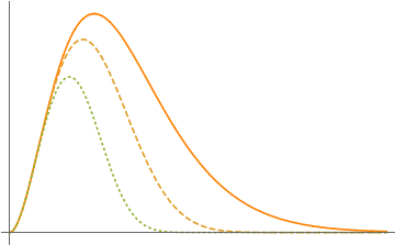
Figure 1: The shape of distribution $f_{\theta}(\omega)$ for three different values of deformation parameter theta: $\theta=0$ (continuous line), $\theta=0.1$ (dashed line) and $\theta=0.2$ (dotted line). In all three cases we fix temperature $T=1$ and parameter $m=1$.

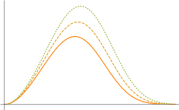
Figure 2: The shape of distribution $f_{\theta}(\omega)$ for three different values of temperature: $T=1$ (continuous line), $T=1.1$ (dashed line) and $T=1.2$ (dotted line). In all three cases we fix the deformation parameter $\theta=1$ and parameter $m=1$.

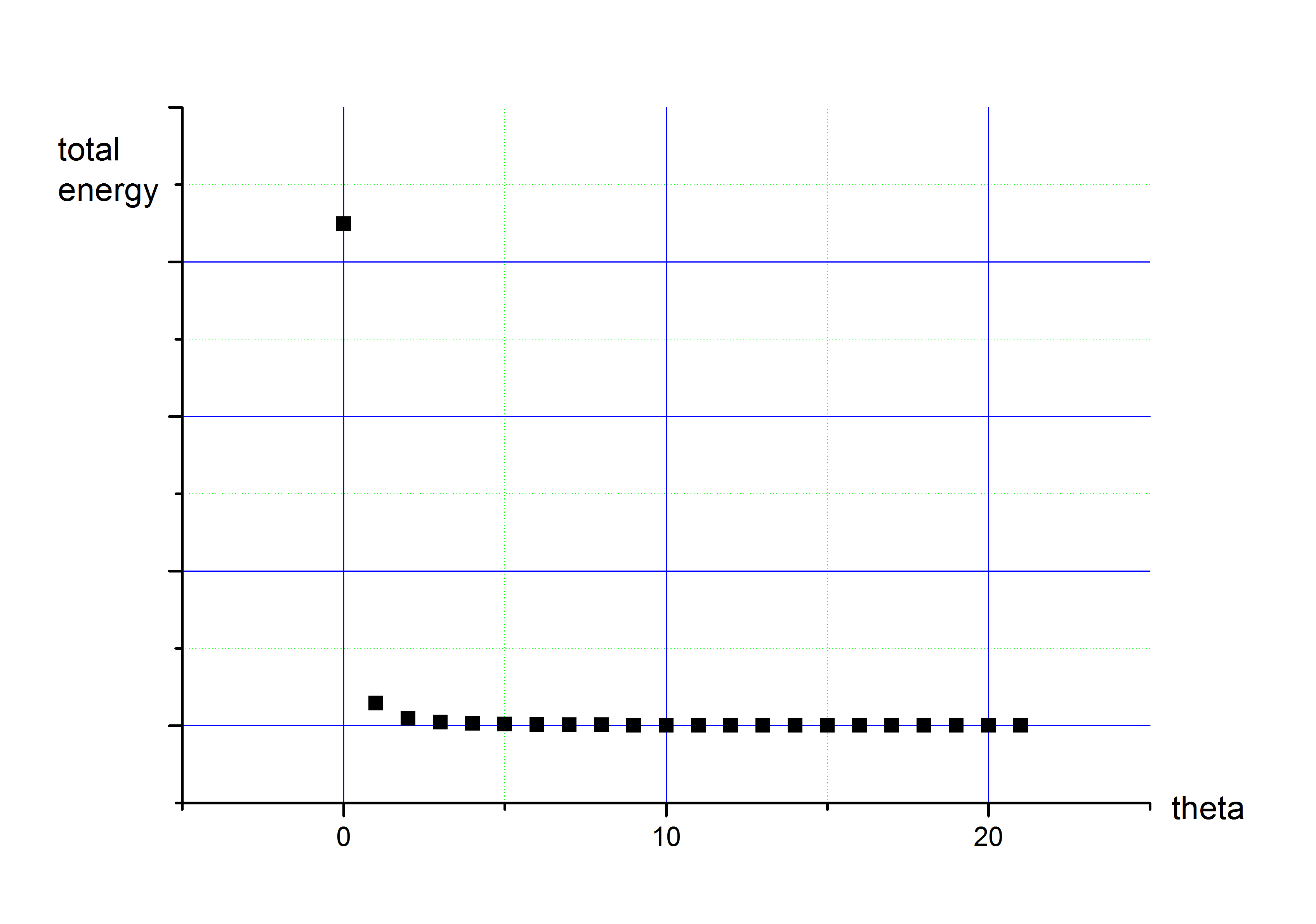
Figure 3: The values of total radiation energy $u_{\theta}$ as a function of the deformation parameter $\theta=0$, 1, 2, $\dots$, 21 for fixed temperature $T=1$.

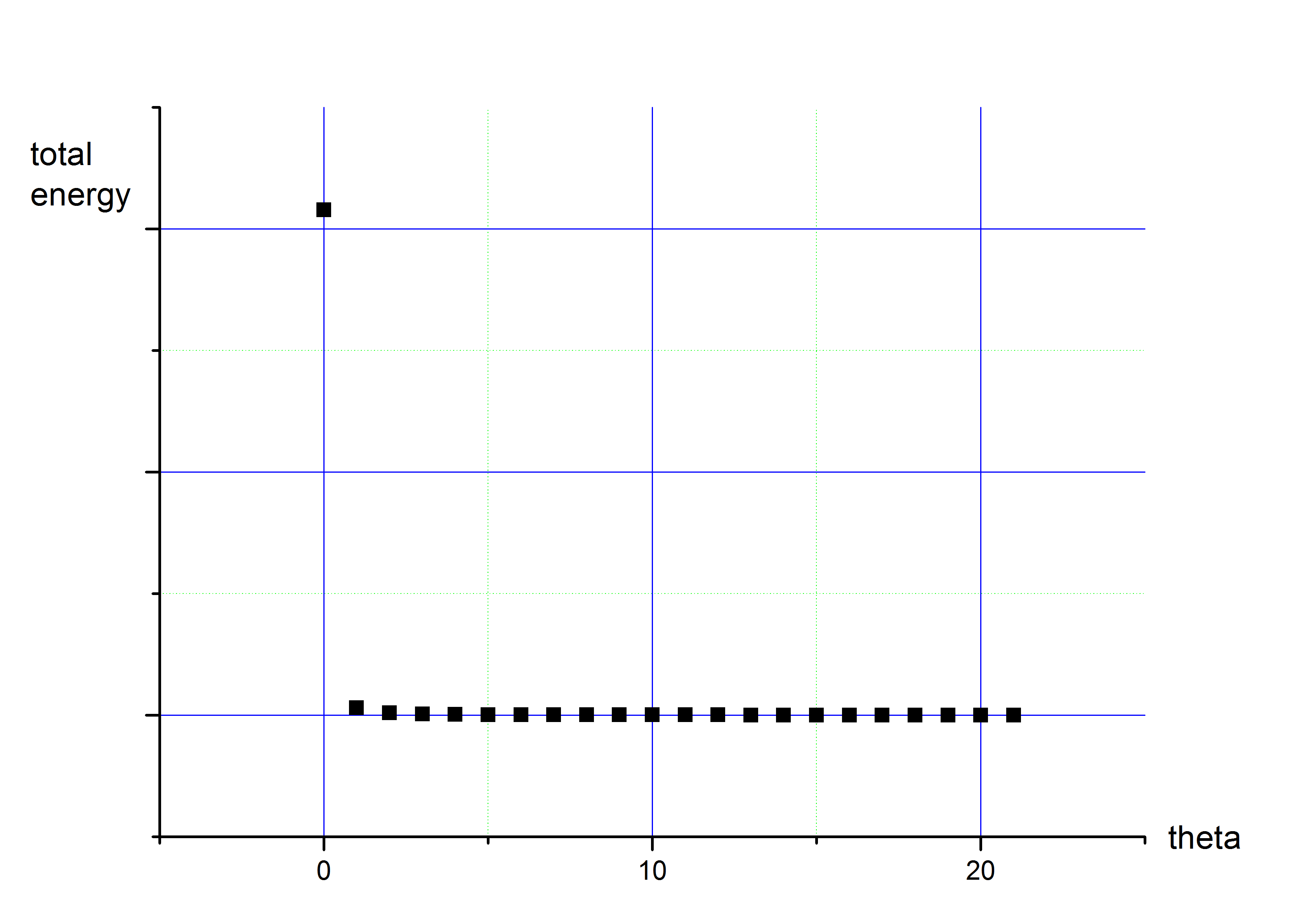
Figure 4: The values of total radiation energy $u_{\theta}$ as a function of the deformation parameter $\theta=0$, 1, 2, $\dots$, 21 for fixed temperature $T=2$.

References

- [1] H.S. Snyder, Phys. Rev. 72, 68 (1947)
- [2] S. Doplicher, K. Fredenhagen, J.E. Roberts, Phys. Lett. B 331, 39 (1994); Comm. Math. Phys. 172, 187 (1995); hep-th/0303037
- [3] A. Kempf and G. Mangano, Phys. Rev. D 55, 7909 (1997); hep-th/9612084
- [4] A. Connes, M.R. Douglas, A. Schwarz, JHEP 9802, 003 (1998); hep-th/9711162
- [5] N. Seiberg and E. Witten, JHEP 9909, 032 (1999); hep-th/9908142
- [6] A. Deriglazov, JHEP 0303, 021 (2003); hep-th/0211105
- [7] S. Ghosh, Phys. Lett. B 648, 262 (2007)
- [8] M. Chaichian, M.M. Sheikh-Jabbari, A. Tureanu, Phys. Rev. Lett. 86, 2716 (2001); hep-th/0010175
- [9] Kh.P. Gnatenko, V.M. Tkachuk, Phys. Lett. A 378, 3509 (2014); arXiv: 1407.6495 [quant-ph]
- [10] P. Kosinski, J. Lukierski, P. Maslanka, Phys. Rev. D 62, 025004 (2000); hep-th/9902037
- [11] M. Chaichian, P. Prešnajder and A. Tureanu, Phys. Rev. Lett. 94, 151602 (2005); hep-th/0409096
- [12] G. Fiore, J. Wess, Phys. Rev. D 75, 105022 (2007); hep-th/0701078
- [13] V. Chari, A. Pressley, ”A Guide to Quantum Groups”, Cambridge University Press, Cambridge, 1994
- [14] L.A. Takhtajan, ”Introduction to Quantum Groups”; in Clausthal Proceedings, Quantum groups 3-28 (see High Energy Physics Index 29 (1991) No. 12256)
- [15] S. Zakrzewski, ”Poisson Structures on the Poincare group”; q-alg/9602001
- [16] Y. Brihaye, E. Kowalczyk, P. Maslanka, ”Poisson-Lie structure on Galilei group”; math/0006167
- [17] M. Daszkiewicz, Mod. Phys. Lett. A27 (2012) 1250083; arXiv: 1205.0319 [hep-th]
- [18] R. Oeckl, J. Math. Phys. 40, 3588 (1999)
- [19] M. Chaichian, P.P. Kulish, K. Nashijima, A. Tureanu, Phys. Lett. B 604, 98 (2004); hep-th/0408069
- [20] M. Daszkiewicz, Mod. Phys. Lett. A 23, 505 (2008); arXiv: 0801.1206 [hep-th]
- [21] J. Lukierski, A. Nowicki, H. Ruegg and V.N. Tolstoy, Phys. Lett. B 264, 331 (1991)
- [22] S. Giller, P. Kosinski, M. Majewski, P. Maslanka and J. Kunz, Phys. Lett. B 286, 57 (1992)
- [23] J. Lukierski and M. Woronowicz, Phys. Lett. B 633, 116 (2006); hep-th/0508083
- [24] O. Ogievetsky, W.B. Schmidke, J. Wess, B. Zumino, Comm. Math. Phys. 150, 495 (1992)
- [25] P. Aschieri, L. Castellani, A.M. Scarfone, Eur. Phys. J. C 7, 159 (1999); q-alg/9709032
- [26] J.M. Romero and J.D. Vergara, Mod. Phys. Lett. A 18, 1673 (2003); hep-th/0303064
- [27] J.M. Romero, J.A. Santiago, J.D. Vergara, Phys. Lett. A 310, 9 (2003); hep-th/0211165
- [28] Y. Miao, X. Wang, S. Yu, Annals Phys. 326, 2091 (2011); arXiv: 0911.5227 [math-ph]
- [29] A. Kijanka, P. Kosinski, Phys. Rev. D 70, 12702 (2004); hep-th/0407246
- [30] M. Daszkiewicz, C.J. Walczyk, Phys. Rev. D 77, 105008 (2008); arXiv: 0802.3575 [math-ph]
- [31] E. Harikumar, A.K. Kapoor, Mod. Phys. Lett. A 25, 2991 (2010); arXiv: 1003.4603 [hep-th]
- [32] P.R. Giri, P. Roy, Eur. Phys.J. C 57, 835 (2008); arXiv: 0803.4090 [hep-th]
- [33] J.D. Anderson, P.A. Laing, E.L. Lau, A.S. Lin, M.M. Nieto, S.G. Turyshev, Phys. Rev. Lett. 81, 2858 (1998); gr-qc/9808081
- [34] O.F. Dayi, A. Jellal, J. Math. Phys. 43, 4592 (2002); hep-th/0111267
- [35] S. Dulat, K. Li, Chin. Phys. C 32, 92 (2008); arXiv: 0802.1118 [math-ph]
- [36] B. Basu, S. Ghosh, Phys. Lett. A 346, 133 (2005); cond-mat/0503266
- [37] A. Kokado, T. Okamura, T. Saito, ”Noncommutative Hall Effect”; hep-th/0210194
- [38] P.R. Giri, P. Roy, Eur. Phys. J. C 57, 835 (2008); arXiv: 0803.4090 [hep-th]
- [39] M. Daszkiewicz, Acta Phys. Polon. B 44, 59 (2013); arXiv: 1302.0827 [hep-th]
- [40] M. Daszkiewicz, Acta Phys. Polon. B 45, 2047 (2014); arXiv: 1412.5922 [hep-th]
- [41] A.M. Fatollahi, M. Hajirahimi, Phys. Lett. B 641, 381 (2006); hep-th/0611225
- [42] A.M. Fatollahi, M. Hajirahimi, Europhys. Lett. 75, 542 (2006); astro-ph/0607257
- [43] M. Planck, Annalen der Physik 4, 553 (1901)
- [44] K. Huang, ”Statistical Mechanics” 2nd ed. John Willey and Sons, 1987