Laguerre polynomial excited coherent states generated by multiphoton catalysis: Nonclassicality and Decoherence

Abstract

We theoretically introduce a new kind of non-Gaussian state—–Laguerre polynomial excited coherent states by using the multiphoton catalysis which actually can be considered as a block comprising photon number operator. It is found that the normalized factor is related to the two-variable Hermite polynomials. We then investigate the nonclassical properties in terms of Mandel’s Q parameter, quadrature squeezing, second correlation, and the negativity of Wigner function (WF). It is shown that all these properties are related to the amplitude of coherent state, catalysis number and unbalanced beam splitter (BS). In particular, the maximum degree of squeezing can be enhanced as catalysis number and keeps a constant for single-photon catalysis. In addition, we examine the effect of decoherence by Wigner function, which show that the negative region, characteristic time of decoherence and structure of WF are affected by catalysis number and unbalanced BS. Our work provides a general analysis about how to prepare theoretically polynomials quantum states.

Keywords: nonclassical property; Laguerre polynomials excitation; squeezing; Wigner function

PACS: 03.65 -a. 42.50.Dv

I Introduction

Nonclassical state has an important role in understanding deeply some fundamental problems in the field of quantum mechanics. In order to realize this purpose, many experimental and theoretical protocols have been proposed to generate and manipulate such nonclassical quantum states 1 ; 2 ; 2a ; 3 ; 4 ; 4a ; 5 ; 6 ; 6a ; 7 . In these protocols, the photon addition $a^{{\dagger}}$, as a non-Gaussian operation, can create a nonclassical state from any classical state 2 ; 7 . In addition, practically realizable non-Gaussian operations including the photon subtraction $a$ or addition $a^{{\dagger}}$ or the superposition of both were used to improve the nonclassicality, the degree of entanglement, the fidelity of continuous variable teleportation, loophole-free tests of Bell’s inequality, and quantum computing, as well as the performance of quantum-key-distribution 3 ; 8 ; 9 ; 10 ; 11 ; 12 ; 13 ; 14 . For example, the quantum commutation rules have been probed experimentally by using addition and subtraction of single photons to/from a light field 4 ; 4a .

In addition, the multi-photon process has experimentally an theoretically attracted much attention 7 ; 15 ; 16 ; 17 ; 18 ; 19 ; 20 ; 21 . For example, the multi-photon excited coherent state has been introduced by Agarwl, and the corresponding nonclassical properties and experimental preparation are discussed by using parametric down-conversion and homodyne tomography technology 7 ; 22 ; 23 ; 24 ; 25 ; 26 ; 27 . Single photon addition is used theoretically to improve the performance of quantum-key-distribution 13 . Recently, multiple-photon subtraction and addition have been used to enhance the degree of entanglement for two-mode squeezed vacuum (TMSV) and the fidelity of teleportation with continuous 19 ; 20 ; 28 ; 29 . It is shown that the highest entanglement, the fidelity and some squeezing properties can be improved for the TMSV with symmetric multi-photon subtraction operations. Both two non-Gaussian operations can actually be realized by using the linear optical elements such as beam splitter and conditional measurement on ancillary outcome, which is probabilistic but more feasible in the laboratory compared with nonlinear process.

On the other hand, it is interesting to notice that Hermite polynomial states can be considered as the minimum uncertain states 30 ; 31 , on which are focused by some researchers 14 ; 32 ; 33 . For instance, a generalized Hermite polynomial’s operation has been theoretically introduced and operated on single-mode squeezed vacuum and coherent state 32 ; 33 , such as $H_{n}\left(Q\right)\left|\alpha\right\rangle$ and $H_{n}\left(\mu a+\nu a^{\dagger}\right)S\left(r\right)\left|0\right\rangle$ where $Q=(a+a^{\dagger})/\sqrt{2}$ is the coordinate operator and $\left|\alpha\right\rangle$ is the Glauber coherent state, and $S\left(r\right)\left|0\right\rangle$ is the single-mode squeezed vacuum. It is found that all these nonclassicalities can be enhanced by Hermite polynomial operation and two adjustable parameters 33 . However, there is no scheme proposed to generate such these polynomial states. The implementation of such non-Gaussian operations is still a very challenging task 34 .

In order to prepare the non-Gaussian states, excepting for photon addition and subtraction or both, the quantum catalysis is also a feasible strategy to generate nonclassical quantum states 35 ; 17 . The analogy to catalysis is to perform a measurement with the same number of photons as ancillary mode on one output, which can generate an effective nonlinearity. In this paper, we shall introduce a new kind of non-Gaussian quantum states—–Laguerre polynomial excited coherent states (LPECSs), which can be produced by using beam splitter and a special conditional measurement (multi-photon catalysis) on one of two outports. Then we investigate the nonclassical properties according to the Mandel’s Q parameter and second-order correlation function, photon-number distribution, squeezing property as well as the Wigner function. Particularly, we also discuss the decoherence effect of thermal channel on the LPECSs by deriving analytically the Wigner function. There is no report about this non-Gaussian state generated by multiphoton catalysis before, including the effect of decoherence on the nonclassicality.

This work is arranged as follows. In Sec. II, we propose the protocol for generating such a kind of non-Gaussian state by using the heralded interference and conditional measurement. In Sec. III, we derive the normalization factor, which is important for further discussing the statistical properties of the state. It is shown that the factor is related to the two-variable Hermite polynomials. In Sec. IV, we present the statistical properties of the state, such as photon-number distribution, squeezing, etc. Secs. V and VI are devoted to investigating the nonclassicality in terms of the negativity of Wigner function without and with the effect of decoherence of the thermal channel, respectively. Our conclusions and discussions are presented in the last section.

II The generation of the LPECSs

The scheme for generating an optical state $\left|\Psi\right\rangle_{out}$ by the heralded interference and conditional measuring $m$ photons is shown in Fig.1. In Fig.1, an arbitrary input pure state $\left|\varphi\right\rangle_{in}$ and an $m-$photon Fock state $\left|m\right\rangle_{a}$ are sent on an asymmetrical beam splitter (BS), and a number measurement is performed on one of the two outports.

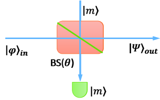
Figure 1: (Color online) An optical state $\left|\Psi\right\rangle_{out}$ is generated by the interference between an arbitrary input pure state $\left|\varphi\right\rangle_{in}$ and an $m-$photon Fock state (at a beam splitter of reflectivity $\left|r\right|^{2}=1-\left|t\right|^{2}$), conditional measuring $m$ photons at one output.

If we have a conditional measurement with $m$ photons at one output port (see Fig.1), then the conditioned state at the other output is given by

$$\left|\Psi\right\rangle_{out}=N_{m}\left.{}_{a}\left\langle m\right|B\left(\theta\right)\left|m\right\rangle_{a}\right.\left|\varphi\right\rangle_{in},$$ (1)

where $N_{m}$ is the normalization factor, and $B\left(\theta\right)=\exp\left\{\theta(a^{\dagger}b-ab^{\dagger})\right\}$ is the BS operator, and $r=\sin\theta$, $t=\cos\theta$. BS operator is actually an entangling operator 36a .When $\theta=\pi/4$, $B\left(\pi/4\right)$ is the symmetrical BS. In order to further obtain the expression in Eq.(1), we first derive the matrix element ${}_{a}\left\langle m\right|B\left(\theta\right)\left|m\right\rangle_{a}$. Using the normal ordering form of $B\left(\theta\right)$ 36 :

$$B\left(\theta\right) =\colon\exp\left\{\left(\cos\theta-1\right)\left(a^{{\dagger}}a+b^{{\dagger}}b\right)\right.$$

$$+\left.\left(a^{\dagger}b-ab^{\dagger}\right)\sin\theta\right\}\colon,$$ (2)

and the coherent state representation of Fock state, i.e.,

$$\left|m\right\rangle=\frac{1}{\sqrt{m!}}\frac{\partial^{m}}{\partial\alpha^{m}}\left.\left\|\alpha\right\rangle\right|_{\alpha=0},\left\|\alpha\right\rangle=\exp\left(\alpha a^{\dagger}\right)\left|0\right\rangle,$$ (3)

we can derive

$$\hat{B}_{m} \equiv\left.{}_{a}\left\langle m\right|B\left(\theta\right)\left|m\right\rangle_{a}\right.$$

$$=\frac{\left(-\cos\theta\right)^{m}}{m!}\colon H_{m,m}\left(b^{{\dagger}}\tan\theta,b\tan\theta\right)\colon e^{b^{{\dagger}}b\ln\cos\theta}$$

$$=\cos^{m}\theta\colon L_{m}\left(b^{{\dagger}}b\tan^{2}\theta\right)\colon e^{b^{{\dagger}}b\ln\cos\theta},$$ (4)

where $L_{m}\left(.\right)$ is the Laguerre polynomials, $H_{m,m}\left(x,y\right)$ is the two-variable Hermite polynomials, and we have used the operator identity $\colon\exp\{\left(e^{\lambda}-1\right)b^{{\dagger}}b\}\colon=e^{\lambda b^{{\dagger}}b}$ and $e^{\lambda b^{{\dagger}}b}be^{-\lambda b^{{\dagger}}b}=e^{-\lambda}b$ and the relation $\left(-1\right)^{m}/m!H_{m,m}\left(x,y\right)=L_{m}\left(xy\right)$. Thus, for any input state, the output state can be expressed as $\left|\Psi\right\rangle_{out}\rightarrow\hat{B}_{m}\left|\varphi\right\rangle_{in}$. It will be convenient to further discuss some properties of the output states by using Eq.(4). From Eq.(4), we can see that the process, accompanying with $m$-photon Fock state input and $m$-photon measured, can be seen as a kind of Laguerre polynomials operation of number operator within normal ordering form.

When the input state $\left|\varphi\right\rangle_{in}$ is the coherent state $\left|z\right\rangle$, then the output state is given by

$$\left|\Psi\right\rangle_{out} =N_{m}\cos^{m}\theta\colon L_{m}\left(b^{{\dagger}}b\tan^{2}\theta\right)\colon e^{b^{{\dagger}}b\ln\cos\theta}\left|z\right\rangle$$

$$=N_{m}e^{-\frac{1}{2}\left|z\right|^{2}\sin^{2}\theta}\cos^{m}\theta L_{m}\left(\mu b^{{\dagger}}\right)\left|z\cos\theta\right\rangle$$

$$\equiv\bar{N}_{m}L_{m}\left(\mu b^{{\dagger}}\right)\left|z\cos\theta\right\rangle,$$ (5)

where we have set $\mu=z\cos\theta\tan^{2}\theta,$ $\bar{N}_{m}=N_{m}\cos^{m}\theta\exp[-\frac{1}{2}\left|z\right|^{2}\sin^{2}\theta]$ and we have used the formula

$$g^{b^{{\dagger}}b}\left|\alpha\right\rangle=\exp\left[\frac{1}{2}\left(g^{2}-1\right)\left|\alpha\right|^{2}\right]\left|g\alpha\right\rangle.$$ (6)

It is clear that Eq.(5) is just the Laguerre polynomials excited coherent state (LPECSs) generated by the condition measurement. Let us note that the scaling $\cos\theta$ of the coherent state $z$ can be understood as a loss process. This character is a result of the process itself. For the case of $\theta=0$ corresponding to the perfect transmission ($t=1,r=0$), we see $\left|\Psi\right\rangle_{out}\rightarrow\left|z\right\rangle$, as expected. When $m=0$, $1$, the output states become $\left|\Psi\right\rangle_{out}=\left|z\cos\theta\right\rangle$, and $\left|\Psi\right\rangle_{out}=\bar{N}_{1}\left(1-\mu b^{{\dagger}}\right)\left|z\cos\theta\right\rangle$, respectively. The former is still a coherent state with a smaller amplitude $z\cos\theta$ comparing with that of the initial input state, which means that even when for instance $m=0$ (without photon detected) the average number of photon at the output is $\left|z\right|^{2}\cos^{2}\theta,$ not $\left|z\right|^{2},$ i.e., the average numbers of photon are not conservation for the input-output state at the process of quantum catalysis; And the latter corresponds to a superposition of coherent state and excited coherent state.

III Normalization of the LPECSs

Next, we derive the normalization of the LPECSs, which is important for discussing the statistical properties of quantum states. Using the normalized condition $1=\left.{}_{out}\left\langle\Psi\right|\left.\Psi\right\rangle_{out}\right.$ and the completeness relation $\int d^{2}\alpha\left|\alpha\right\rangle\left\langle\alpha\right|/\pi=1$ of coherent state, as well as

$$\left\langle z\cos\theta\right|\left.\alpha\right\rangle=\exp\left\{-\frac{\left|z\right|^{2}}{2}\cos^{2}\theta-\frac{1}{2}\left|\alpha\right|^{2}+z^{\ast}\alpha\cos\theta\right\},$$ (7)

we can derive

$$\bar{N}_{m}^{-2} =\left\langle z\cos\theta\right|L_{m}\left(\mu^{\ast}b\right)L_{m}\left(\mu b^{{\dagger}}\right)\left|z\cos\theta\right\rangle$$

$$=\int\frac{d^{2}\alpha}{\pi}\left|L_{m}\left(\mu^{\ast}\alpha\right)\right|^{2}\left|\left\langle z\cos\theta\right|\left.\alpha\right\rangle\right|^{2}$$

$$=\int\frac{d^{2}\alpha}{\pi}\left|L_{m}\left(\mu^{\ast}\alpha\right)\right|^{2}e^{-\left|z\right|^{2}\cos^{2}\theta-\left|\alpha\right|^{2}+\left(z^{\ast}\alpha+z\alpha^{\ast}\right)\cos\theta}.$$ (8)

Using the sum representation of Laguerre polynomial

$$L_{m}\left(x\right)=\sum_{l=0}^{m}\binom{m}{l}\frac{(-1)^{l}}{l!}x^{l},$$ (9)

we can rewrite Eq.(8) as the following form

$$\bar{N}_{m}^{-2} =\sum_{l,k=0}^{m}\binom{m}{l}\binom{m}{k}\frac{(-1)^{l+k}}{l!k!}\mu^{k}\mu^{\ast l}$$

$$\times e^{-\left|z\right|^{2}\cos^{2}\theta}\int\frac{d^{2}\alpha}{\pi}\alpha^{\ast k}\alpha^{l}e^{-\left|\alpha\right|^{2}+\left(z^{\ast}\alpha+z\alpha^{\ast}\right)\cos\theta}$$

$$=\sum_{l,k=0}^{m}\binom{m}{l}\binom{m}{k}\frac{(-1)^{k}\mu^{k}\mu^{\ast l}}{l!k!}H_{k,l}\left(z^{\ast}\cos\theta,-z\cos\theta\right),$$ (10)

where we have used the following integration formula

$$H_{m,n}\left(\xi,\eta\right)=(-1)^{n}e^{\xi\eta}\int\frac{d^{2}z}{\pi}z^{n}z^{\ast m}e^{-\left|z\right|^{2}+\xi z-\eta z^{\ast}}.$$ (11)

Eq.(10) is the analytical expression of normalization factor for the output state $\left|\Psi\right\rangle_{out}$, which is related to the two-variable Hermite polynomials. $\bar{N}_{m}^{-2}$ is a real number which can be seen directly from Eq.(8). In particular, when $m=1$ corresponding to the single-photon catalysis, we have $\bar{N}_{1}^{-2}=(1-\left|z\right|^{2}\sin^{2}\theta)^{2}+\left|z\right|^{2}\cos^{2}\theta\tan^{4}\theta$ which is in accordance with 17 .

In a similar way to deriving Eq.(10), we can calculate the matrix element $\left\langle b^{q}b^{{\dagger}p}\right\rangle$ as

$$\left\langle b^{q}b^{{\dagger}p}\right\rangle =\sum_{l,k=0}^{m}\binom{m}{l}\binom{m}{k}\frac{(-1)^{q+k}}{l!k!}\mu^{k}\mu^{\ast l}$$

$$\times\bar{N}_{m}^{2}H_{k+p,l+q}\left(z^{\ast}\cos\theta,-z\cos\theta\right),$$ (12)

which will be often used in the next calculation for discussing the nonclassical properties of the LPECSs.

IV Nonclassical properties of the LPECSs

In this section, we shall discuss the nonclassical properties of the LPECSs by using Mandel’s $\mathfrak{Q}$ parameter and second-order correlation function, photon-number distribution, as well as squeezing property.

IV.1 Mandel’s $\mathfrak{Q}$ parameter

First, let us examine the sub-Possion statistical property using the Mandel $\mathfrak{Q}$-parameter 37 , whose definition can be given by

$$\mathfrak{Q} =\frac{\left\langle\left(b^{{\dagger}}b\right)^{2}\right\rangle-\left\langle b^{{\dagger}}b\right\rangle^{2}}{\left\langle b^{{\dagger}}b\right\rangle}-1$$

$$=\frac{\left\langle b^{2}b^{{\dagger}2}\right\rangle-\left\langle bb^{{\dagger}}\right\rangle^{2}-2\left\langle bb^{{\dagger}}\right\rangle+1}{\left\langle bb^{{\dagger}}\right\rangle-1}.$$ (13)

The quantum state shall satisfy the sub-Poissonian statistics when the condition $\mathfrak{Q}<0$ is achieved. The super-Poissonian, Poissonian statistics correspond to $\mathfrak{Q}>0$ and $\mathfrak{Q}=0$, respectively. For simplicity, here we have converted the expression of $\mathfrak{Q}$ to the anti-normally ordering form. Using Eq.(12), we can get the analytical expression of $\mathfrak{Q}$ but do not give them here due to its long and cumbersome.

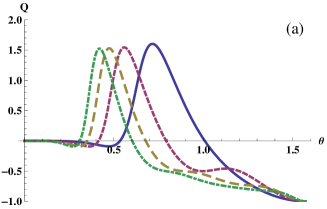
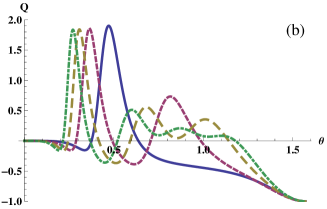
Figure 2: (Color online) The $\mathfrak{Q}$-parameter as the function of ${\small\theta}$ for several different values $m=1,2,3,4,$ and (a) ${\small z}$=1, (b) ${\small z}$=2. The highest peaks from right to left correspond to m=1,2,3,4, respectively.

In order to see clearly the variation of Mandel’s $\mathfrak{Q}$ parameter with the input amplitude $z$ and the asymmetrical BS ($\theta$), we plot the $\mathfrak{Q}$ parameter in Fig. 2 as the function of $\theta$ for some several different values of $z$ and $m$. Here, for simplicity, we take $z$ as a real number. From Fig. 2, we can clearly see that, for a given small $z$ value ($z=1$), the $\mathfrak{Q}$ parameter can be negative ($m\neq 0$) when $\theta$ is less than a certain threshold value or when $\theta$ is larger than a one. Both threshold values decrease as $m$ increases; while for a large value $z$($z=2$), the main peaks become more narrow and the corresponding threshold values become smaller than those for the case of small value of input amplitude. These imply that the output state presents obvious nonclassicality which can be modulated the transmission factor.

IV.2 Second-Order Correlation Function

Notice that the condition $\mathfrak{Q}<0$ is actually a sufficient condition indicating the nonclassical property. That is to say, when $\mathfrak{Q}>0$ the state also maybe nonclassical. Next, we will further discuss the second-order correlation function for the LPECSs, which is typically used to find the statistical character of intensity fluctuations. The second-order correlation function is defined by 38

$$g^{(2)}=\frac{\left\langle b^{{\dagger}2}b^{2}\right\rangle}{\left\langle b^{{\dagger}}b\right\rangle^{2}}=\frac{\left\langle b^{2}b^{{\dagger}2}-4bb^{{\dagger}}+2\right\rangle}{\left(\left\langle bb^{{\dagger}}\right\rangle-1\right)^{2}}.$$ (14)

Theoretically, using the result $\left\langle b^{q}b^{{\dagger}p}\right\rangle$ in Eq.(12) we can get the analytical expression of $g^{(2)}$.

In Fig. 3, we plot the $g^{(2)}$ correlation function as the function of $\theta$ for some several different values of $\left|z\right|^{2}$ and $m$. From Fig. 3 we can see that there are some regions which present clearly the antibunching effect with $g^{(2)}<1$, bunching effect with $1<g^{(2)}\leqslant 2$ and super-bunching effect with $2<g^{(2)}$ 39 . The antibunching effect, a nonclassical indicator, can be observed for both high and low reflectivities (see Fig. 3 (a)). The main peaks become more narrow and the maximal values of peaks become smaller than those for the small amplitude case. The latter is different from the case of $\mathfrak{Q}$-parameter. In addition, the positions of peaks move to the left as the increasing $m$. For instance, for $\left|z\right|^{2}=1$, the peaks corresponding to $m=1,2,3,4$ are centered around $\theta=0.68,0.53,0.45,0.39$, which attain the corresponding measured values of $g^{(2)}=6.93,6.83,6.76,6.72$, respectively. It is clear that all these values of peaks are over the limit of thermal states which is not a signature of nonclassicality; For $m=1$, in the regions of $\theta<0.47$ and $\theta>0.90$, the signature of nonclassicality appears and becomes more clear in the region of $\theta>0.90$ with the increasing $\theta$. These cases are similar for $m=2,3,4$.

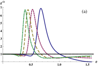
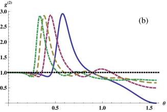
Figure 3: (Color online) The second order correlation function $g^{(2)}$as the function of ${\small\theta}$ for several different values $m=1,2,3,4,$ and (a) $\left|{\small z}\right|^{2}$=1, (b) $\left|{\small z}\right|^{2}$=2. The highest peaks from right to left correspond to m=1,2,3,4, respectively. When $m=0,$$g^{(2)}=1$ corresponding to the classical bound.

IV.3 Photon number distribution

Next, let us consider the photon-number distribution (PND) of the LPECSs. In this field, the PND of finding $n$ photons can be calculated as

$$p_{n}=\left|\bar{N}_{m}\right|^{2}\left|\left\langle n\right|L_{m}\left(\mu b^{{\dagger}}\right)\left|z\cos\theta\right\rangle\right|^{2}.$$ (15)

In order to obtain the explicit form of $p_{n}$, we first evaluate the matrix element $\left\langle n\right|L_{m}\left(\mu b^{{\dagger}}\right)\left|z\cos\theta\right\rangle$. Using the coherent representation of number state in Eq.(3) and the sum representation of Laguerre polynomials in Eq. (9), we have

$$\left\langle n\right|L_{m}\left(\mu b^{{\dagger}}\right)\left|z\cos\theta\right\rangle$$

$$=\frac{1}{\sqrt{n!}}\frac{\partial^{n}}{\partial\alpha^{\ast n}}L_{m}\left(\mu\alpha^{\ast}\right)\left\langle\alpha\right\|\left|z\cos\theta\right\rangle_{\alpha^{\ast}=0}$$

$$=\frac{e^{-\frac{1}{2}\left|z\right|^{2}\cos^{2}\theta}}{\sqrt{n!}}\frac{\partial^{n}}{\partial\alpha^{\ast n}}L_{m}\left(\mu\alpha^{\ast}\right)\left.e^{\alpha^{\ast}z\cos\theta}\right|_{\alpha^{\ast}=0}$$

$$=\frac{e^{-\frac{1}{2}\left|z\right|^{2}\cos^{2}\theta}}{\sqrt{n!}}\sum_{l=0}^{m}\binom{m}{l}\frac{(-\mu)^{l}}{l!}\frac{\partial^{n}}{\partial\alpha^{\ast n}}\alpha^{\ast l}\left.e^{\alpha^{\ast}z\cos\theta}\right|_{\alpha^{\ast}=0}$$

$$=\frac{e^{-\frac{1}{2}\left|z\right|^{2}\cos^{2}\theta}}{\sqrt{n!}}\sum_{l=0}^{m}\binom{m}{l}\binom{n}{l}(-\mu)^{l}\left(z\cos\theta\right)^{n-l},$$ (16)

thus the PND is given by

$$p_{n} =\frac{\left|\bar{N}_{m}\right|^{2}}{n!}e^{-\left|z\right|^{2}\cos^{2}\theta}$$

$$\times\left|\sum_{l=0}^{m}\binom{m}{l}\binom{n}{l}(-\mu)^{l}\left(z\cos\theta\right)^{n-l}\right|^{2}.$$ (17)

It is easy to see that Eq.(17) just reduces to the PND of the coherent state $\left|z\cos\theta\right\rangle$ when $m=0$, i.e., $p_{n}=\frac{1}{n!}e^{-\left|z\right|^{2}\cos^{2}\theta}\left|z\cos\theta\right|^{2n}$, as expected.

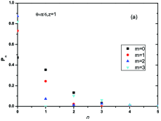
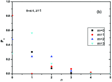
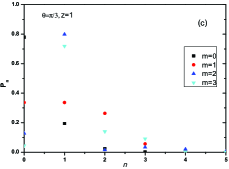
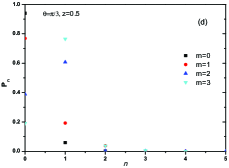
Figure 4: (Color online) The photon-number distribution of the LPECSs as a function of $n$ for several different parameters $\theta$, $m$ and $z$. (a) $\theta=\pi/6,z=1;$ (b) $\theta=\pi/4,z=1;$ (c) $\theta=\pi/3,z=1;$ (d) $\theta=\pi/3,z=0.5.$

In Fig. 4, the PND is plotted for several different parameters $\theta$, $m$ and $z$, from which we can see that (i) the peak of PND is mainly located at $n=0$ for the case of $m=0$ and different values of $\theta$ and $z$ (see Figs. 4.(a)-(d)); (ii) by modulating the order $m$ of Laguerre polynomials, we may change the position and value of the peak. For example, the maximum values of peaks at $n=0$ increase as $m$ increase (see Fig. 4(a)); (iii) for $m=1,2,3$, the PND is mainly distributed at $n=1$ and the maximum values of peaks modulated by beam splitter ($\theta$), which implies that we can prepare single photon Fock state by this conditional measurement for a given amplitude of input coherent state; for instance, when $\theta=\pi/4$ and $m=3$, we can get a single-photon in a success probability of $0.57$ (see Fig. 4(b)), while for $\theta=\pi/3$ the probabilities are 0.80 and 0.72 for $m=2,3$ (see Fig. 4(c)), respectively. This is to say, we can achieve the single-photon at a smaller measured $m$ when increasing the value of $\theta$ for a given $z$; (iv) for a small amplitude value of z (see Fig. 4(d)), we can increase the measured $m$ to obtain the single-photon in a higher probability (say when $m=2,3$, probability=0.61 and 0.77). Thus we can not only modify the PND but also achieve single-photon Fock state by the quantum catalysis rather than photon-subtraction (photon-loss).

IV.4 Squeezing properties

Now, we investigate the squeezing properties of the LPECSs via the quadrature variance $\left(\triangle Q\right)^{2}<1$ or $\left(\triangle P\right)^{2}<1$ which indicates the squeezing or sub-Poissonian statistics. The quadrature components of the optical field is given by $Q=(b+b^{{\dagger}})/\sqrt{2}$ and $P=(b-b^{{\dagger}})/(i\sqrt{2})$. Thus the quadrature variances can be expressed as the following anti-normally ordering forms

$$\left(\triangle Q\right)^{2} =\left\langle Q^{2}\right\rangle-\left\langle Q\right\rangle^{2}$$

$$=\frac{1}{2}\left\{\left\langle b^{2}\right\rangle-\left\langle b\right\rangle^{2}+\left\langle b^{{\dagger}2}\right\rangle-\left\langle b^{{\dagger}}\right\rangle^{2}\right.$$

$$\left.+2\left\langle bb^{{\dagger}}\right\rangle-2\left\langle b\right\rangle\left\langle b^{{\dagger}}\right\rangle-1\right\},$$ (18)

and

$$\left(\triangle P\right)^{2} =\left\langle P^{2}\right\rangle-\left\langle P\right\rangle^{2}$$

$$=\frac{1}{2}\left\{-\left\langle b^{2}\right\rangle+\left\langle b\right\rangle^{2}-\left\langle b^{{\dagger}2}\right\rangle+\left\langle b^{{\dagger}}\right\rangle^{2}\right.$$

$$\left.+2\left\langle bb^{{\dagger}}\right\rangle-2\left\langle b\right\rangle\left\langle b^{{\dagger}}\right\rangle-1\right\}.$$ (19)

Using Eq.(12) we can get the analytical expressions for the variance of the quadratures, but are not given here. Next, we shall discuss the squeezing properties by numerical calculation.

In Fig. 5, we plot these optimal quadrature variances as a function of the input amplitudes for several different values of $m$ by minimizing variances $\left(\triangle Q\right)^{2}$ over $\theta$ from 0 to $\pi/2$. Here, we take a logarithmic scale, i.e. units of dB whose definition is given by dB$[Q]=10\log_{10}[\left(\triangle Q\right)^{2}/\left(\triangle Q\right)_{vac}^{2}]$ and dB$[P]=10\log_{10}[\left(\triangle P\right)^{2}/\left(\triangle P\right)_{vac}^{2}],$ where $\left(\triangle Q\right)_{vac}^{2}$ and $\left(\triangle P\right)_{vac}^{2}$ corresponding to the vacuum variances of $1/2$ for our definition of quadrature components. In Fig. 5(a), it is clearly seen that (i) when $m=1$, the optimal squeezing is 1.249 dB below the shot-noise limit and it is independent of the input amplitude $z$; (ii) the optimal values of squeezing or the minimum variances monotonously increase as $m$ for a given amplitude $z$, and decrease as $z$ for $m=2,3,4$. These results indicate that the squeezing can be enhanced by increasing measured $m$ photons or reducing the amplitude $z$. Fig. 5(b) shows the $\theta$ values corresponding to the largest squeezing effect as a function of $z$, from which we can see that the $\theta$ value decreases as $m$ for a given $z$ and monotonously decreases as $z$ for a given $m$.

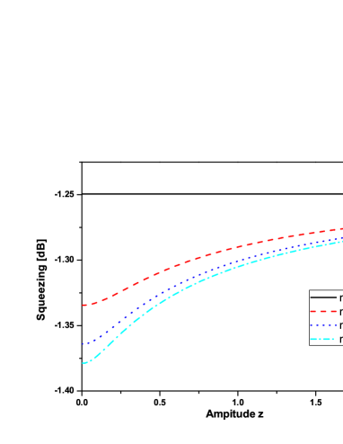
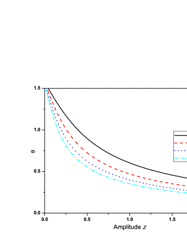
Figure 5: (Color online) (a) The optimal squeezing effect as a function of the input amplitude $z$ by minimizing the variances of quadrature component $Q$over $\theta$; (b) the $\theta$values corresponding to the optimal squeezing effect as a function of $z$.

Next, we further consider the squeezing properties of the LPECSs by introducing another quadrature operator $Q_{\varphi}=ae^{-i\varphi}+a^{\dagger}e^{i\varphi}$. Thus the squeezing can be characterized by the minimum value $\left\langle\triangle^{2}Q_{\varphi}\right\rangle$ $<1$ with respect to $\varphi$, or by the normal ordering form $\left\langle\colon\triangle^{2}Q_{\varphi}\colon\right\rangle<0$. Upon expanding the terms of $\left\langle\colon\triangle^{2}Q_{\varphi}\colon\right\rangle$, one can minimize its value over the whole angle $\varphi$. The optimized nonclassical depth over the phases is found to be 40

$$S_{opt}=-2\left|\left\langle a^{\dagger 2}\right\rangle-\left\langle a^{\dagger}\right\rangle^{2}\right|+2\left\langle aa^{\dagger}\right\rangle-2\left|\left\langle a^{\dagger}\right\rangle\right|^{2}-2.$$ (20)

The negative value of $S_{opt}$ in the range $\left[-1,\text{ }0\right)$ implies squeezing (or nonclassical). Using Eq.(12) we can get the expression of $S_{opt}$. In particular, when $m=0$ (the case of coherent output), $S_{opt}=0$, as expected. In Fig. 6 we plot the $S_{opt}$ as a function of $\theta$ for some different values of $m$ and $z$, from which we can see that there is a region of $\theta$ for representing the negative value of $S_{opt},$ and the region becomes smaller with the increasing $m$ and $z.$ For a given $m$ or $z$, the region becomes narrower for a bigger $z$ or $m$. For more discussions about higher-order nonclassical effects of quantum state, we refer to Refs.41 ; 42 ; 43 ; 44 .

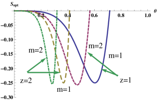
Figure 6: (Color online) The degree of squeezing Sopt of the LPECSs as the function of $\theta$ for different values of $m$and $z$.

V Wigner distribution of the LPECSs

In this section, we shall discuss the quasi-probability distribution, Wigner function, whose negativity may be considered as a good indicator of the nonclassicality. For the single-mode case, the Wigner function can be calculated as

$$W\left(\gamma\right)=\mathtt{tr}(\rho\Delta(\gamma)),$$ (21)

where $\Delta(\gamma)$ is the single-mode Wigner operator 45 , defined by

$$\Delta(\gamma)=e^{2\left|\gamma\right|^{2}}\int\frac{d^{2}\alpha}{\pi^{2}}\left|\alpha\right\rangle\left\langle-\alpha\right|e^{-2(\alpha\gamma^{\ast}-\gamma\alpha^{\ast})},$$ (22)

and $\left|z\right\rangle=\exp\left(zb^{{\dagger}}-z^{\ast}b\right)\left|0\right\rangle$ is Glauber coherent state. Substituting Eqs.(5) and (22) into Eq.(21) and using Eq.(7), the Wigner function of can be derived as

$$W_{m}\left(\gamma\right)=\left|\bar{N}_{m}\right|^{2}e^{2\left|\gamma\right|^{2}-\left|z\right|^{2}\cos^{2}\theta}\Theta\left(\mu,\mu^{\ast}\right),$$ (23)

where

$$\Theta\left(\mu,\mu^{\ast}\right) =\int\frac{d^{2}\alpha}{\pi^{2}}L_{m}\left(-\mu\alpha^{\ast}\right)L_{m}\left(\mu^{\ast}\alpha\right)$$

$$\times e^{-\left|\alpha\right|^{2}+\alpha\left(z^{\ast}\cos\theta-2\gamma^{\ast}\right)-\alpha^{\ast}\left(z\cos\theta-2\gamma\right)}.$$ (24)

It is easy to see that the Wigner function $W\left(\gamma\right)$ is a real number in phase space, since $\Theta^{\ast}\left(\mu,\mu^{\ast}\right)=\Theta\left(\mu,\mu^{\ast}\right)$.

Furthermore, using Eqs.(9) and (11) we can finally obtain the Wigner function

$$W_{m}\left(\gamma\right)=W_{0}\left(\gamma\right)F_{m}\left(\gamma\right),$$ (25)

where $W_{0}\left(\gamma\right)=1/\pi\exp\{-2\left|\gamma-z\cos\theta\right|^{2}\}$ is just the Wigner function of coherent state $\left|z\cos\theta\right\rangle$, and the non-Gaussian item $F_{m}\left(\gamma\right)$ is defined by

$$F_{m}\left(\gamma\right) =\left|\bar{N}_{m}\right|^{2}\sum_{j,l=0}^{m}\frac{\mu^{l}\mu^{\ast j}}{l!j!}\binom{m}{j}\binom{m}{l}$$

$$\times H_{l,j}\left(z^{\ast}\cos\theta-2\gamma^{\ast},z\cos\theta-2\gamma\right),$$ (26)

which is from the presence of conditionally measured $m$ photons. In particular, when $m=1,$ then we have

$$F_{1}\left(\gamma\right) =\left|\bar{N}_{1}\right|^{2}\{1+\left|\mu\right|^{2}(1-\left|z\cos\theta-2\gamma\right|^{2})$$

$$+[\mu\left(z^{\ast}\cos\theta-2\gamma^{\ast}\right)+c.c]\}.$$ (27)

The negative region of Wigner function will be decided by $F_{1}\left(\gamma\right)<0$.

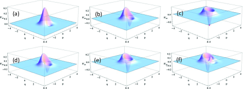
Figure 7: (Color online) The Wigner function distribution in phase space with z=1 for some different values of m and $\theta$. The first and second rows correspond to m=1,2, respectively. And $\theta\$are equal to $\pi/5,\pi/4,\pi/3$from left to right for each column.

In Fig. 7, we plot the Wigner distributions in phase space for several different parameter values of $m$ and $\theta$ with $z=1$, from which it is clearly seen that there are some obvious negative regions of the Wigner function in the phase space which is an indicator of the nonclassicality of the state. Furthermore, these negative areas are modulated not only by $m$, but also by $\theta$. For example, for a given $\theta=\pi/5$ (see Figs. 7 (a) and (d)), there is a bigger negative volume of the Wigner function for the case of $m=2$ than that for $m=1$; and for a given $m=1$, the negative volume of the Wigner function becomes bigger as $\theta$ increases (see Fig.7 (a)-(c)). Actually, the structure of the Wigner function will be affected by the input amplitude $z$. In order to clearly see these above points, we further quantify the negative volume of the Wigner function, defined by $\delta=\frac{1}{2}[\int_{-\infty}^{\infty}dqdp\left|W(q,p)\right|-1]$ with $\gamma=(q+ip)/\sqrt{2}$. In table I, we present some values of negative volume of the Wigner function for different $m$, $\theta$, and $z$. It is clearly seen that the effects on the nonclassicality are different due to the changing of parameters $m$, $\theta$, and $z$.

TABLE I: Negative volume $\delta$ of the WF
case	z=1			z=2
case	$\theta$=$\frac{\pi}{5}$	$\theta$=$\frac{\pi}{4}$	$\theta$=$\frac{\pi}{3}$	$\theta$=$\frac{\pi}{5}$	$\theta$=$\frac{\pi}{4}$	$\theta$=$\frac{\pi}{3}$
m=1	0.023	0.115	0.205	0.163	0.115	0.122
m=2	0.116	0.180	0.207	0.149	0.271	0.297
m=3	0.164	0.188	0.212	0.242	0.307	0.412

VI Decoherence in thermal environment

In this section, we consider the decoherence of the LPECSs by analytically deriving the Wigner function in thermal environment. When the quantum state evolves in a thermal environment associated with Born-Markivian approximation, the evolution of density operator can be described by the following master equation 46

$$\frac{d\rho}{dt} =\kappa(\tilde{n}+1)(2a\rho a^{\dagger}-a^{\dagger}a\rho-\rho a^{\dagger}a)$$ (28)

$$+\kappa\tilde{n}\left(2a^{\dagger}\rho a-aa^{\dagger}\rho-\rho aa^{\dagger}\right),$$

where $\kappa$ denotes the dissipative coefficient and $\tilde{n}$ represents the average thermal photon number of the lossy channel. Using the entangled state representation, we have derived the sum representation of Klaus operator and the evolution of the Wigner function governed by Eq.(28) 47 ; 48 . The latter is given by

$$W\left(\beta,\beta^{\ast},t\right)=\frac{2}{(2\tilde{n}+1)T}\int\frac{d^{2}\gamma}{\pi}W\left(\gamma,\gamma^{\ast}\right)e^{-2\frac{|\beta-\gamma e^{-\kappa t}|^{2}}{(2\tilde{n}+1)T}},$$ (29)

where $W\left(\gamma,\gamma^{\ast}\right)$ is the initial Wigner function and $T=1-e^{-2\kappa t}$. Then substituting Eq.(23) into Eq.(29) and using the following integration formula

$$\int\frac{d^{2}z}{\pi}e^{-\zeta\left|z\right|^{2}+\xi z+\eta z^{\ast}}=\frac{1}{\zeta}e^{\frac{\xi\eta}{\zeta}},\text{Re}\left(\zeta\right)>0,$$ (30)

we finally obtain

$$W\left(\beta,\beta^{\ast},t\right)=W_{0}\left(\beta,t\right)F_{m}\left(\beta,t\right),$$ (31)

where $W_{0}\left(\beta,t\right)=\frac{1}{\pi A}\exp\{-\allowbreak 2\left|\beta-\bar{z}e^{-\kappa t}\right|^{2}/A\}$ with $A=2\tilde{n}T+1\$and $\bar{z}=z\cos\theta$ is the evolution of Wigner function of coherent state $\left|z\cos\theta\right\rangle$ in thermal channel, and

$$F_{m}\left(\beta,t\right) =\left|\bar{N}_{m}\right|^{2}\sum_{j,l=0}^{m}\frac{\mu^{l}\mu^{\ast j}}{l!j!}\binom{m}{j}\binom{m}{l}\left(\sqrt{\frac{B}{A}}\right)^{l+j}$$

$$\times H_{l,j}\left(\frac{\bar{z}^{\ast}B-2\beta^{\ast}e^{-\kappa t}}{\sqrt{AB}},\frac{\bar{z}B-2\beta e^{-\kappa t}}{\sqrt{AB}}\right)$$

$$\left(B=e^{-2\kappa t}-(2\tilde{n}+1)T\right).$$ (32)

In particular, when $t=0$ Eqs.(31) and (32) just reduce to Eqs.(25) and (26), respectively.

In Fig. 8, we take the case with $m=1$ and $z=1$ as well as $\theta=\pi/3$ as an example for the evolution of Wigner function. From Fig. 8, due to the presence of decoherence, the negative region of Wigner function gradually disappears with the incasement of $\kappa t$. In addition, the characteristic time $\kappa t_{c}$, which means that there is always negative region for Wigner function in phase space when the decay time is less than $\kappa t_{c}$, is dependent not only on the catalytic photon number $m$, but also on the reflectivity of unbalanced BS. In order to see clearly this point, we plot the minimum negative values of Wigner function as a function of decay time $\kappa t$ in Fig. 9, from which it is clear that the minimum negative decreases monotonously as $\kappa t$; in addition, for instance, the characteristics times for $m=1$ are about $0.20,0.27$ and $0.30$ corresponding to $\theta=\pi/5,\pi/4,\pi/3$, respectively. There is a longer characteristic time for $\theta=\pi/3$ than that for $\theta=\pi/5,\pi/4.$ This point can be understood like that: because the case of $\theta=\pi/3$ has a higher reflectivity than that of $\theta=\pi/5,\pi/4$, thus the output state presents more properties of number state. Actually, the output state can be considered as the superposition of coherent state and number state in a certain form.

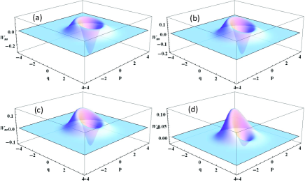
Figure 8: (Color online) The evolution of Wigner function distribution in phase space with $m=1,$ $\tilde{n}=0$. (a)-(d) $\kappa t=0,0.05,0.1,0.2.$

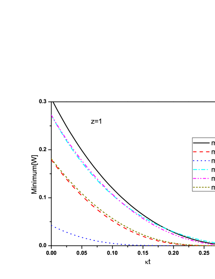
Figure 9: (Color online) The minimum value of negative Wigner function distribution in phase space as the function of the decay time $\kappa t$ for $m=1,2,$ $\tilde{n}=0$ and $z=1,$ $\theta=\pi/5,\pi/4,\pi/3.$

VII Conclusion

In this paper, we proposed a new kind of non-Gaussian state—-Laguerre polynomial excited coherent state by using multiphoton catalysis which is proposed firstly by Lvovsky and Mlynek. It is shown that the multiphoton catalysis can actually be seen as a block comprising photon number operator. We then considered the nonclassical properties of the LPECs when considering the coherent state as inputs. It is found that the state can present sub-Possion statistics, antibunching effect and squeezing behavior. All these properties can be modulated by the amplitude of coherent state, catalysis number and unbalanced BS. In particular, the maximum squeezing for the case of $m=1$ is kept to be constant ($\sim$1.249dB) by optimizing over unbalanced BS. The maximum squeezing can be improved by increasing $m$ and reducing the amplitude of coherent state. In addition, we also examined the decoherence behavior of the LPECs according to the negativity of Wigner function. It is found that the negative region, characteristic time of decoherence and structure of Wigner function are affected by catalysis number and unbalanced BS.

Here the generation of Laguerre polynomials excited state is just an example for opening the way approaching a series of non-Gaussian quantum state. Actually, by different herald inputs and different measurements, we can achieve some other non-Gaussian states such as Hermite polynomials excited squeezed states, etc. Our current work provides a general analysis about how to prepare theoretically such polynomials quantum states.

It would be interesting to extend this work to multi-mode case including how to realize the entanglement distillation and improve the fidelity of teleportation. On the other hand, non-Gaussian quantum states have a wide application in quantum information and quantum computation 49 . For example, by using photon-subtraction operator, a scheme is proposed to improve the performance of entanglement-based continuous-variable quantum-key-distribution protocol 12 . It is found that the subtraction operation can increase the secure distance and tolerable excess noise of the entanglement-based scheme, as well as the corresponding prepare-and-measure scheme. Recently, for another example, the single-photon-added coherent state has been used in quantum key distribution 13 . It is shown that the single-photon-added coherent source can greatly exceed all other existing sources in both BB84 protocol and the recently proposed measurement-device-independent quantum key distribution. These investigations are good examples for showing that it is possible to enhance the performance in the field of quantum information by preparing various non-Gaussian states. Thus, the applications of such non-Gaussian states including the LPECSs with continuous-variable in quantum information could be paid attention in the future.

Acknowledgments: This work is supported by a grant from the Qatar National Research Fund (QNRF) under the NPRP project 7-210-1-032. L. Y. Hu is supported by the China Scholarship Council (CSC) and the National Natural Science Foundation of China (Nos.11264018 and 11264015), as well as the Natural Science Foundation of Jiangxi Province (No. 20152BAB212006), the Research Foundation of the Education Department of Jiangxi Province of China (no GJJ14274).

References

- (1) D. Bouwmeester, A. K. Ekert, A. Zeilinger, The Physics of Quantum Information. Springer, Berlin (2000).
- (2) M. S. Kim, “Recent developments in photon-level operations on travelling light fields,” J. Phys. B 41, 133001-133018 (2008), and references therein.
- (3) A. Zavatta, V. Parigi, M. Bellini, “Experimental nonclassicality of single-photon-added thermal light states,” Phys. Rev. A 75, 052106 (2007).
- (4) A. Ourjoumtsev, A. Dantan, R. Tualle-Brouri, and P. Grangier, “Increasing Entanglement between Gaussian States by Coherent Photon Subtraction,” Phys. Rev. Lett. 98, 030502 (2007).
- (5) M. S. Kim, H. Jeong, A. Zavatta, V. Parigi, M. Bellini, “Scheme for Proving the Bosonic Commutation Relation Using Single-Photon Interference,” Phys. Rev. Lett. 101, 260401 (2008).
- (6) V. Parigi, A. Zavatta, M. S. Kim, and M. Bellini, “Probing quantum commutation rules by addition and subtraction of single photons to/from a light Ffield,” Science 317, 1890-1893 (2007).
- (7) S. Y. Lee, J. Park, S. W. Ji, C. H. Raymond Ooi, and H. W. Lee, “Nonclassicality generated by photon annihilation-then-creation and creation-then-annihilation operations,” J. Opt. Soc. Am. B 26, 1532-1537 (2009).
- (8) T. Opatrný, G. Kurizki and D.-G. Welsch, “Improvement on teleportation of continuous variables by photon subtraction via conditional measurement,” Phys. Rev. A 61, 032302 (2000).
- (9) T. Bartley, P. Crowley, A. Datta, J. Nunn, L. Zhang, and I. Walmsley, “Strategies for enhancing quantum entanglement by local photon subtraction,” Phys. Rev. A 87 022313 (2013).
- (10) G. S. Agarwal and K. Tara, “Nonclassical properties of states generated by the excitations on a coherent state,” Phys. Rev. A 43, 492 (1991).
- (11) D. E. Browne, J. Eisert, S. Scheel, and M. B. Plenio, “Driving non-Gaussian to Gaussian states with linear optics,” Phys. Rev. A 67, 062320-1-9 (2003).
- (12) H. Nha and H. J. Carmichael, “Proposed Test of Quantum Nonlocality for Continuous Variables,” Phys. Rev. Lett. 93, 020401-020404 (2004).
- (13) R. García-Patrón, J. Fiurášek, N. J. Cerf, J. Wenger, R. Tualle-Brouri, and P. Grangier, “Proposal for a Loophole-Free Bell Test Using Homodyne Detection,” Phys. Rev. Lett. 93, 130409 (2004).
- (14) S. D. Bartlett and B. C. Sanders, “Universal continuous-variable quantum computation: Requirement of optical nonlinearity for photon counting,” Phys. Rev. A 65, 042304 (2002).
- (15) Y. Yang, F. L. Li, “Nonclassicality of photon-subtracted and photon-added-then-subtracted Gaussian states,” J. Opt. Soc. Am. B, 26, 830-835 (2009).
- (16) P. Huang, G. Q. He, J. Fang, and G. H. Zeng, “Performance improvement of continuous-variable quantum key distribution via photon subtraction,” Phys. Rev. A 87, 012317 (2013).
- (17) D. Wang, M. Li, F. Zhu, Z. Q. Yin, W. Chen, Z. F. Han, G. C. Guo, and Q. Wang, “Quantum key distribution with the single-photon-added coherent source,” Phys. Rev. A 90, 062315 (2014).
- (18) Z. Wang, H. M. Li, and H. C Yuan, “Quasi-probability distributions and decoherence of Hermite-excited squeezed thermal states,” J. Opt. Soc. Am. B 31, 2163-2174 (2014).
- (19) M. Cooper, L. J. Wright, C. Soller, and B. J. Smith, “Experimental generation of multi-photon Fock states,” Optics Express 21, 5309-5317 (2013).
- (20) M. Yukawa, K. Miyata, T. Mizuta, H. Yonezawa, P. Marek, R. Filip, and A. Furusawa, “Generating superposition of up-to three photons for continuous variable quantum information processing, Optics Express, 21, 5529-5535 (2013).
- (21) T. J. Bartley, G. Donati, J. B. Spring, X. M. Jin, M. Barbieri, A. Datta, B. J. Smith, and I. A. Walmsley, “Multiphoton state engineering by heralded interference between single photons and coherent states,” Phys. Rev. A 86 043820 (2012).
- (22) E. Bimbard, N. Jain, A. MacRae and A. I. Lvovsky, Quantum-optical state engineering up to the two-photon level, Nature Photonics 4, 243-247 (2010).
- (23) C. Navarrete-Benlloch, R. Garcia-Patron, J. H. Shapiro, and N. J. Cerf, “Enhancing quantum entanglement by photon addition and subtraction,” Phys. Rev. A 86, 012328 (2012).
- (24) S. Wang, L. L. Hou, X. F. Chen, and X. F. Xu “Continuous-variable quantum teleportation with non-Gaussian entangled states generated via multiple-photon subtraction and addition,” Phys. Rev. A 91 063832 (2015).
- (25) J Fiurášek, “Engineering quantum operations on traveling light beams by multiple photon addition and subtraction,” Phys. Rev. A 80, 053822 (2009).
- (26) S. Sivakumar, “Studies on nonlinear coherent states,” J. Opt. B: Quantum Semiclass. Opt. 2, R61 (2000).
- (27) V V. Dodonov, M. A. Marchiolli, Y. A. Korennoy, V. I. Man’ko, Y. A. Moukhin, “Dynamical squeezing of photon-added coherent states,” Phys. Rev. A 58, 4087 (1998).
- (28) A. Zavatta, S. Viciani, and M. Bellini, “Quantum-to-classical transition with single-photon-added coherent states of light.,” Science 306, 660-662 (2004).
- (29) A. Zavatta, S. Viciani, and M. Bellini, “Single-photon excitation of a coherent state: Catching the elementary step of stimulated light emission,” Phys. Rev. A 72, 023820 (2005).
- (30) D. Kalamidas, C. C. Gerry and A. Benmoussa, “Proposal for generating a two-photon added coherent state via down-conversion with a single crystal,” Phys. Lett. A, 372, 1937-1940 (2008).
- (31) L. Y. Hu and H. Y. Fan, “Statistical properties of photon-added coherent state in a dissipative channel,” Phys. Scr. 79, 035004 (2009).
- (32) L. Y. Hu and Z. M. Zhang, “Statistical properties of coherent photon-added two-mode squeezed vacuum and its inseparability,” J. Opt. Soc. Am. B 30, 518-529 (2013).
- (33) L. Y. Hu, F. Jia and Z. M. Zhang, “Entanglement and nonclassicality of photon-added two-mode squeezed thermal state,” J. Opt. Soc. Am. B 29, 1456-1464 (2012).
- (34) J. A. Bergou, H. Mark, and D. Q. Yu, “Minimum uncertainty states for amplitude-squared squeezing: Hermite polynomial states” Phys. Rev. A 43, 515 (1999).
- (35) H. Y. Fan and X. Ye, “Hermite polynomial states in two-mode Fock space,” Phys. Lett. A 175, 387-390 (1993).
- (36) G. Ren, J. M. Du, H. J. Yu, and Y. J. Xu, “Nonclassical properties of Hermite polynomial’s coherent state,” J. Opt. Soc. Am. B 29, 3412 (2012).
- (37) S. Y. Liu, Y. Z. Li, L. Y. Hu, J. H. Huang, X. X. Xu and X. Y. Tao, “Nonclassical properties of Hermite polynomial excitation on squeezed vacuum and its decoherence in phase-sensitive reservoirs,” Laser Phys. Lett. 12, 045201 (2015).
- (38) K. Park, P. Marek, and R. Filip, “Nonlinear potential of a quantum oscillator induced by single photons,” Phys. Rev. A 90, 013804 (2014).
- (39) A. I. Lvovsky and J. Mlynek, “Quantum-Optical Catalysis: Generating Nonclassical States of Light by Means of Linear Optics,” Phys. Rev. Lett. 88, 250401 (2002).
- (40) R. Tahira, M. Ikram, H. Nha, and M. S. Zubairy, “Entanglement of Gaussian states using a beam splitter,” Phys. Rev. A 79, 023816 (2009).
- (41) F. Jia, X. X. Xu, C. J. Liu, J. H. Huang, L. Y. Hu, H. Y. Fan, “Decompositions of beam splitter operator and its entanglement function,” Acta Phys. Sin. 63, 220301 (2014).
- (42) L. Mandel, “Sub-Poissonian photon statistics in resonance fluorescence,” Opt. Lett. 4, 205–207 (1979).
- (43) M. O. Scully and M. S. Zubairy, Quantum Optics, Cambridge University Press, (Cambridge, UK) (1997).
- (44) T. Sh. Iskhakov, A. M. Pérez, K. Yu. Spasibko, M. V. Chekhova, and G. Leuchs, “Superbunched bright squeezed vacuum state,” Opt Lett. 37, 1919-1921 (2012).
- (45) C. K. Hong and L. Mandel, “Generation of higher-order squeezing of quantum electromagnetic field,” Phys. Rev. A 32, 974-982 (1985).
- (46) M. Hillery, “Amplitude-squared squeezing of the electromagnetic field,” Phys. Rev. A 36, 3796–3802 (1987).
- (47) C. T. Lee, “Higher-order criteria for nonclassical effects in photon statistics,” Phys. Rev. A 41, 1721-1723 (1990).
- (48) Z. M. Zhang, L. Xu, J. L. Chai, and F. L. Li, “A new kind of higher-order squeezing of radiation field,” Phys. Lett. A 150, 27-30 (1990).
- (49) C. K. Hong and L. Mandel, “Higher-order squeezing of a quantum field,” Phys. Rev. Lett. 54, 323-325 (1985).
- (50) Hong-yi Fan, H. R. Zaidi, “Application of IWOP technique to the generalized Weyl correspondence,” Phys. Lett. A 124, 303-307 (1987).
- (51) C. W. Gardiner and P. Zoller, Quantum Noise (Springer-Verlag, 2000).
- (52) H. Y. Fan and L. Y. Hu, “Operator-sum representation of density operators as solutions to master obtained via the entangled state approach,” Mod. Phys. Lett. B 22, 2435-2468 (2008).
- (53) L.-Y. Hu and H.-Y. Fan, “Time evolution of Wigner function in laser process derived by entangled state representation,” Opt. Commun. 282, 4379-4383 (2009).
- (54) H. Jeong and T. C. Ralph, Quantum Information with Continuous Variables of Atoms and Light, edited by N. J. Cerf, G. Leuchs, and E. S. Polzik (Imperial College Press, London, 2005).