Reduction of Nondeterministic Tree Automata

Abstract

We present an efficient algorithm to reduce the size of nondeterministic tree automata, while retaining their language. It is based on new transition pruning techniques, and quotienting of the state space w.r.t. suitable equivalences. It uses criteria based on combinations of downward and upward simulation preorder on trees, and the more general downward and upward language inclusions. Since tree-language inclusion is EXPTIME-complete, we describe methods to compute good approximations in polynomial time.

We implemented our algorithm as a module of the well-known libvata tree automata library, and tested its performance on a given collection of tree automata from various applications of libvata in regular model checking and shape analysis, as well as on various classes of randomly generated tree automata. Our algorithm yields substantially smaller and sparser automata than all previously known reduction techniques, and it is still fast enough to handle large instances.

1 Introduction

Background. Tree automata are a generalization of word automata that accept trees instead of words [13]. They have many applications in model checking [6, 5, 11], term rewriting [14], and related areas of formal software verification, e.g., shape analysis [3, 19, 17]. Several software packages for manipulating tree automata have been developed, e.g., MONA [8], Timbuk [15], Autowrite [14] and libvata [21], on which other verification tools like Forester [22] are based.

For nondeterministic automata, many questions about their languages are computationally hard. The language universality, equivalence and inclusion problems are PSPACE-complete for word automata and EXPTIME-complete for tree automata [13]. However, recently techniques have been developed that can solve many practical instances fairly efficiently. For word automata there are antichain techniques [2], congruence-based techniques [9] and techniques based on generalized simulation preorders [12]. The antichain techniques have been generalized to tree automata in [10, 20] and implemented in the libvata library [21]. Performance problems also arise in computing the intersection of several languages, since the product construction multiplies the numbers of states.

Automata Reduction. Our goal is to make tree automata more computationally tractable in practice. We present an efficient algorithm for the reduction of nondeterministic tree automata, in the sense of obtaining a smaller automaton with the same language, though not necessarily with the absolute minimal possible number of states. (In general, there is no unique nondeterministic automaton with the minimal possible number of states for a given language, i.e., there can be several non-isomorphic nondeterministic automata of minimal size. This holds even for word automata.) The reason to perform reduction is that the smaller reduced automaton is more efficient to handle in a subsequent computation. Thus there is an algorithmic tradeoff between the effort for reduction and the complexity of the problem later considered for this automaton. The main applications of reduction are the following: (1) Helping to solve hard problems like language universality/equivalence/inclusion. (2) If automata undergo a long chain of manipulations/combinations by operations like union, intersection, projection, etc., then intermediate results can be reduced several times on the way to keep the automata within a manageable size. (3) There are fixed-parameter tractable problems (e.g., in model checking where an automaton encodes a logic formula) where the size of one automaton very strongly influences the overall complexity, and must be kept as small as possible.

Our contribution. We present a reduction algorithm for nondeterministic tree automata. (The tool is available for download [7].) It is based on a combination of new transition pruning techniques for tree automata, and quotienting of the state space w.r.t. suitable equivalences. The pruning techniques are related to those presented for word automata in [12], but significantly more complex due to the fundamental asymmetry between the upward and downward directions in trees.

Transition pruning in word automata [12] is based on the observation that certain transitions can be removed (a.k.a pruned) without changing the language, because other ‘better’ transitions remain. One defines some strict partial order (p.o.) between transitions and removes all transitions that are not maximal w.r.t. this order. A strict p.o. between transitions is called good for pruning (GFP) iff pruning w.r.t. it preserves the language of the automaton. Note that pruning reduces not only the number of transitions, but also, indirectly, the number of states. By removing transitions, some states may become ‘useless’, in the sense that they are unreachable from any initial state, or that it is impossible to reach any accepting state from them. Such useless states can then be removed from the automaton without changing its language. One can obtain computable strict p.o. between transitions by comparing the possible backward- and forward behavior of their source- and target states, respectively. For this, one uses computable relations like backward/forward simulation preorder and approximations of backward/forward trace inclusion via lookahead- or multipebble simulations. Some such combinations of backward/forward trace/simulation orders on states induce strict p.o. between transitions that are GFP, while others do not [12]. However, there is always a symmetry between backward and forward, since finite words can equally well be read in either direction.

This symmetry does not hold for tree automata, because the tree branches as one goes downward, while it might ‘join in’ side branches as one goes upward. While downward simulation preorder (resp. downward language inclusion) between states in a tree automaton is a direct generalization of forward simulation preorder (resp. forward language inclusion) on words, the corresponding upward notions do not correspond to backward on words. Comparing upward behavior of states in tree automata depends also on the branches that ‘join in’ from the sides as one goes upward in the tree. Thus upward simulation/language inclusion is only defined relative to a given other relation that compares the downward behavior of states ‘joining in’ from the sides [1]. So one speaks of “upward simulation of the identity relation” or “upward simulation of downward simulation”. When one studies strict p.o. between transitions in tree automata in order to check whether they are GFP, one has combinations of three relations: the source states are compared by an upward relation $X(Y)$ of some downward relation $Y$, while the target states are compared w.r.t. some downward relation $Z$ (where $Z$ can be, and often must be, different from $Y$). This yields a richer landscape, and many counter-intuitive effects.

We provide a complete picture of which combinations of upward/downward simulation/trace inclusions are GFP on tree automata; cf. Figure 4. Since tree-(trace)language inclusion is EXPTIME-complete [13], we describe methods to compute good approximations of them in polynomial time. Finally, we also generalize results on quotienting of tree automata [18] to larger relations, such as approximations of trace inclusion.

We implemented our algorithm [7] as a module of the well-known libvata [21] tree automaton library, and tested its performance on a given collection of tree automata from various applications of libvata in regular model checking and shape analysis, as well as on various classes of randomly generated tree automata. Our algorithm yields substantially smaller automata than all previously known reduction techniques (which are mainly based on quotienting). Moreover, the thus obtained automata are also much sparser (i.e., use fewer transitions per state and less nondeterministic branching) than the originals, which yields additional performance advantages in subsequent computations.

2 Trees and Tree Automata

Trees. A ranked alphabet $\Sigma$ is a set of symbols together with a function $\#:\Sigma\rightarrow\mathbb{N}_{0}$. For $a\in\Sigma$, $\#{(a)}$ is called the rank of $a$. For $n\geq 0$, we denote by $\Sigma_{n}$ the set of all symbols of $\Sigma$ which have rank $n$.

We define a node as a sequence of elements of $\mathbb{N}$, where $\varepsilon$ is the empty sequence. For a node $v\in\mathbb{N}^{*}$, any node $v^{\prime}$ s.t. $v=v^{\prime}v^{\prime\prime}$, for some node $v^{\prime\prime}$, is said to be a prefix of $v$, and if $v^{\prime\prime}\neq\varepsilon$ then $v^{\prime}$ is a strict prefix of $v$. For a node $v\in\mathbb{N}^{*}$, we define the $i$-th child of $v$ to be the node $vi$, for some $i\in\mathbb{N}$. Given a ranked alphabet $\Sigma$, a tree over $\Sigma$ is defined as a partial mapping $t:\mathbb{N}^{*}\rightarrow\Sigma$ such that for all $v\in\mathbb{N}^{*}$ and $i\in\mathbb{N}$, if $vi\in dom(t)$ then (1) $v\in dom(t)$, and (2) $\#(t(v))\geq i$. In this paper we consider only finite trees.

Note that the number of children of a node $v$ may be smaller than $\#(t(v))$. In this case we say that the node is open. Nodes which have exactly $\#(t(v))$ children are called closed. Nodes which do not have any children are called leaves. A tree is closed if all its nodes are closed, otherwise it is open. By $\mathbb{C}(\Sigma)$ we denote the set of all closed trees over $\Sigma$ and by $\mathbb{T}(\Sigma)$ the set of all trees over $\Sigma$. A tree $t$ is linear iff every node in $dom(t)$ has at most one child.

The subtree of a tree $t$ at $v$ is defined as the tree $t_{v}$ such that $dom(t_{v})=\{v^{\prime}\mid vv^{\prime}\in dom(t)\}$ and $t_{v}(v^{\prime})=t(vv^{\prime})$ for all $v^{\prime}\in dom(t_{v})$. A tree $t^{\prime}$ is a prefix of $t$ iff $dom(t^{\prime})\subseteq dom(t)$ and for all $v\in dom(t^{\prime})$, $t^{\prime}(v)=t(v)$. For $t\in\mathbb{C}(\Sigma)$, the height of a node $v$ of $t$ is given by the function $h$: if $v$ is a leaf then $h(v)=1$, otherwise $h(v)=1+max(h(v1)),\ldots,h(v\#(t(v))))$. We define the height of a tree $t\in\mathbb{C}(\Sigma)$ as $h(\epsilon)$, i.e., as the number of levels of $t$.

Tree automata, top-down. A (finite, nondeterministic) top-down tree automaton (TDTA) is a quadruple $A=(\Sigma,Q,\delta,I)$ where $Q$ is a finite set of states, $I\subseteq Q$ is a set of initial states, $\Sigma$ is a ranked alphabet, and $\delta\subseteq Q\times\Sigma\times Q^{+}$ is the set of transition rules. A TDTA has an unique final state, which we represent by $\psi$. The transition rules satisfy that if $\langle q,a,\psi\rangle\in\delta$ then $\#(a)=0$, and if $\langle q,a,q_{1}\ldots q_{n}\rangle\in\delta$ (with $n>0$) then $\#(a)=n$.

A run of $A$ over a tree $t\in\mathbb{T}(\Sigma)$ (or a $t$-run in $A$) is a partial mapping $\pi:\mathbb{N}^{*}\rightarrow Q$ such that $v\in dom(\pi)$ iff either $v\in dom(t)$ or $v=v^{\prime}i$ where $v^{\prime}\in dom(t)$ and $i\leq\#(t(v^{\prime}))$. Further, for every $v\in dom(t)$, there exists either a) a rule $\langle q,a,\psi\rangle$ such that $q=\pi(v)$ and $a=t(v)$, or b) a rule $\langle{q},{a},q_{1}\dotsc q_{n}\rangle$ such that $q=\pi(v)$, $a=t(v)$, and $q_{i}=\pi(vi)$ for each $i:1\leq i\leq\#(a)$. A leaf of a run $\pi$ on $t$ is a node $v\in dom(\pi)$ such that $vi\in dom(\pi)$ for no $i\in\mathbb{N}$. We call it dangling if $v\not\in dom(t)$. Intuitively, the dangling nodes of a run over $t$ are all the nodes which are in $\pi$ but are missing in $t$ due to it being incomplete. Notice that dangling leaves of $\pi$ are children of open nodes of $t$. The prefix of depth $k$ of a run $\pi$ is denoted $\pi_{k}$. Runs are always finite since the trees we are considering are finite.

We write $t\stackrel{{\scriptstyle\pi}}{{\Longrightarrow}}q$ to denote that $\pi$ is a $t$-run of $A$ such that $\pi(\epsilon)=q$. We use $t\Longrightarrow q$ to denote that such run $\pi$ exists. A run $\pi$ is accepting if $t\stackrel{{\scriptstyle\pi}}{{\Longrightarrow}}q\in I$. The downward language of a state $q$ in $A$ is defined by $D_{A}(q)=\{t\in\mathbb{C}(\Sigma)\mid t\Longrightarrow q\}$, while the language of $A$ is defined by $L(A)=\bigcup_{q\in I}D_{A}(q)$. The upward language of a state $q$ in $A$, denoted $U_{A}(q)$, is then defined as the set of open trees $t$, such that there exists an accepting $t$-run $\pi$ with exactly one dangling leaf $v$ s.t. $\pi(v)=q$. We omit the $A$ subscript notation when it is implicit which automaton we are considering.

In the related literature, it is common to define a tree automaton bottom-up, reading a tree from the leaves to the root [13, 10, 20]. A bottom-up tree automaton (BUTA) can be obtained from a TDTA by reversing the direction of the transition rules and by swapping the roles between the initial states and the final states. See Appendix 0.A for an example of a tree automaton presented in both BUTA and TDTA form.

3 Simulations and Trace Inclusions

We consider different types of relations on states of a TDTA which under-approximate language inclusion. Note that words are but a special case of trees where every node has only one child, i.e., words are linear trees. Downward simulation/trace inclusion on TDTA corresponds to direct forward simulation/trace inclusion in special case of word automata, and upward corresponds to backward [12].

Forward simulation on word automata. Let $A=(\Sigma,Q,\delta,I,F)$ be a NFA. A direct forward simulation $\mathrel{D}$ is a binary relation on $Q$ such that if $q\mathrel{D}r$, then

1. $q\in F\Longrightarrow r\in F$, and

2. for any $\langle q,a,q^{\prime}\rangle\in\delta$, there exists $\langle r,a,r^{\prime}\rangle\in\delta$ such that $q^{\prime}\mathrel{D}r^{\prime}$.

The set of direct forward simulations on $A$ contains ${\it id}$ and is closed under union and transitive closure. Thus there is a unique maximal direct forward simulation on $A$, which is a preorder. We call it the direct forward simulation preorder on $A$ and write $\sqsubseteq^{\mathsf{di}}$.

Forward trace inclusion on word automata. Let $A=(\Sigma,Q,\delta,I,F)$ be a NFA and $w=\sigma_{1}\sigma_{2}\ldots\sigma_{n}\in\Sigma^{*}$ a word of length $n$. A trace of $A$ on $w$ (or a $w$-trace) starting at $q$ is a sequence of transitions $\pi=q_{0}\stackrel{{\scriptstyle\sigma_{1}}}{{\rightarrow}}q_{1}\stackrel{{\scriptstyle\sigma_{2}}}{{\rightarrow}}\cdots\stackrel{{\scriptstyle\sigma_{n}}}{{\rightarrow}}q_{n}$ such that $q_{0}=q$. The direct forward trace inclusion preorder $\subseteq^{di}$ is a binary relation on $Q$ such that $q\subseteq^{di}r$ iff

1. $(q\in F\Longrightarrow r\in F)$, and

2. for every word $w=\sigma_{1}\sigma_{2}\ldots\sigma_{n}\in\Sigma^{*}$ and for every $w$-trace (starting at $q$)
   $\pi_{q}=q\stackrel{{\scriptstyle\sigma_{1}}}{{\rightarrow}}q_{1}\stackrel{{\scriptstyle\sigma_{2}}}{{\rightarrow}}\cdots\stackrel{{\scriptstyle\sigma_{n}}}{{\rightarrow}}q_{n}$, there exists a $w$-trace (starting at $r$) $\pi_{r}=r\stackrel{{\scriptstyle\sigma_{1}}}{{\rightarrow}}r_{1}\stackrel{{\scriptstyle\sigma_{2}}}{{\rightarrow}}\cdots\stackrel{{\scriptstyle\sigma_{n}}}{{\rightarrow}}r_{n}$ such that ($q_{i}\in F\Longrightarrow r_{i}\in F$) for each $i:1\leq i\leq n$.

Since $\pi_{r}$ is required to preserve the acceptance of the states in $\pi_{q}$, trace inclusion is a strictly stronger notion than language inclusion (see Figure 7 in Appendix 0.A).
Downward simulation on tree automata. Let $A=(\Sigma,Q,\delta,I)$ be a TDTA. A downward simulation $D$ is a binary relation on $Q$ such that if $q\mathrel{D}r$, then

1. $(q=\psi\Longrightarrow r=\psi)$, and

2. for any $\langle{q},{a},q_{1}\dotsc q_{n}\rangle\in\delta$, there exists $\langle{r},{a},r_{1}\dotsc r_{n}\rangle\in\delta$ s.t. $q_{i}\,D\,r_{i}$ for $i:1\leq i\leq n$.

Since the set of all downward simulations on $A$ is closed under union and under reflexive and transitive closure (cf. Lemma 4.1 in [18]), it follows that there is one unique maximal downward simulation on $A$, and that relation is a preorder. We call it the downward simulation preorder on $A$ and write $\sqsubseteq^{\mathsf{dw}}$.

Downward trace inclusion on tree automata. Let $A=(\Sigma,Q,\delta,I)$ be a TDTA. The downward trace inclusion preorder $\subseteq^{\mathsf{dw}}$ is a binary relation on $Q$ s.t. $q\subseteq^{\mathsf{dw}}r$ iff for every tree $t\in\mathbb{C}(\Sigma)$ and for every $t$-run $\pi_{q}$ with $\pi_{q}(\epsilon)=q$ there exists another $t$-run $\pi_{r}$ s.t.

1. $\pi_{r}(\epsilon)=r$, and

2. ($\pi_{q}(v)=\psi\,\Longrightarrow\,\pi_{r}(v)=\psi$) for each leaf node $v\in dom(t)$.

Generally, one way of making downward language inclusion on the states of an automaton coincide with downward trace inclusion is by modifying the automaton to guarantee that 1) there is one unique final state which has no outgoing transitions, 2) from any other state, there is a path ending in that final state. Note that in a TDTA these two conditions are automatically satisfied: 1) since the final state is reached after reading a leaf of the tree, and 2) because only complete trees are in the language of the automaton. Thus, in a TDTA, downward language inclusion and downward trace inclusion coincide.

Backward simulation on word automata. Let $A=(\Sigma,Q,\delta,I,F)$ be a NFA. A backward simulation $\mathrel{B}$ is a binary relation on $Q$ s.t. if $q\mathrel{B}r$, then

1. ($q\in F\,\Longrightarrow\,r\in F$) and ($q\in I\,\Longrightarrow\,r\in I$), and

2. for any $\langle q^{\prime},a,q\rangle\in\delta$, there exists $\langle r^{\prime},a,r\rangle\in\delta$ s.t. $q^{\prime}\mathrel{B}r^{\prime}$.

Like for forward simulation, there is a unique maximal backward simulation on $A$, which is a preorder. We call it the backward simulation preorder on $A$ and write $\sqsubseteq^{\mathsf{bw}}$.

Backward trace inclusion on word automata. Let $A=(\Sigma,Q,\delta,I,F)$ be a NFA and $w=\sigma_{1}\sigma_{2}\ldots\sigma_{n}\in\Sigma^{*}$ a word of length $n$. A $w$-trace of $A$ ending at $q$ is a sequence of transitions $\pi=q_{0}\stackrel{{\scriptstyle\sigma_{1}}}{{\rightarrow}}q_{1}\stackrel{{\scriptstyle\sigma_{2}}}{{\rightarrow}}\cdots\stackrel{{\scriptstyle\sigma_{n}}}{{\rightarrow}}q_{n}$ such that $q_{n}=q$. The backward trace inclusion preorder $\subseteq^{\mathsf{bw}}$ is a binary relation on $Q$ such that $q\subseteq^{\mathsf{bw}}r$ iff

1. ($q\in F\Longrightarrow r\in F$) and ($q\in I\Longrightarrow r\in I$), and

2. for every word $w=\sigma_{1}\sigma_{2}\ldots\sigma_{n}\in\Sigma^{*}$ and for every $w$-trace (ending at $q$) $\pi_{q}=q_{0}\stackrel{{\scriptstyle\sigma_{1}}}{{\rightarrow}}q_{1}\stackrel{{\scriptstyle\sigma_{2}}}{{\rightarrow}}\cdots\stackrel{{\scriptstyle\sigma_{n}}}{{\rightarrow}}q$, there exists a $w$-trace (ending at $r$) $\pi_{r}=r_{0}\stackrel{{\scriptstyle\sigma_{1}}}{{\rightarrow}}r_{1}\stackrel{{\scriptstyle\sigma_{2}}}{{\rightarrow}}\cdots\stackrel{{\scriptstyle\sigma_{n}}}{{\rightarrow}}r$ such that ($q_{i}\in F\Longrightarrow r_{i}\in F\,\land\;q_{i}\in I\Longrightarrow r_{i}\in I$) for each $i:1\leq i\leq n$.

Upward simulation on tree automata. Let $A=(\Sigma,Q,\delta,I)$ be a TDTA. Given a binary relation $\mathrel{R}$ on $Q$, an upward simulation $U(R)$ induced by $\mathrel{R}$ is a binary relation on $Q$ such that if $q\mathrel{U(R)}r$, then

1. $(q=\psi\Longrightarrow r=\psi)$ and $(q\in I\Longrightarrow r\in I)$, and

2. for any $\langle{q^{\prime}},{a},q_{1}\dotsc q_{n}\rangle\in\delta$ with $q_{i}=q$ (for some $i:1\leq i\leq n$), there exists
   $\langle{r^{\prime}},{a},r_{1}\dotsc r_{n}\rangle\in\delta$ such that $r_{i}=r$, $q^{\prime}\mathrel{U(R)}r^{\prime}$ and $q_{j}\mathrel{R}r_{j}$ for each $j:1\leq j\neq i\leq n$.

Similarly to the case of downward simulation, for any given relation $R$, there is a unique maximal upward simulation induced by $R$ which is a preorder (cf. Lemma 4.2 in [18]). We call it the upward simulation preorder on $A$ induced by $R$ and write $\sqsubseteq^{\mathsf{up}}\!\!\!\;\!\!(R)$.

Upward trace inclusion on tree automata. Let $A=(\Sigma,Q,\delta,I)$ be a TDTA. Given a binary relation $\mathrel{R}$ on $Q$, the upward trace inclusion preorder $\subseteq^{\mathsf{up}}\!\!\!\;\!(R)$ induced by $\mathrel{R}$ is a binary relation on $Q$ such that $q\subseteq^{\mathsf{up}}\!\!\!\;\!(\mathrel{R})\,r$ iff $(q=\psi\Longrightarrow r=\psi)$ and the following holds: for every tree $t\in T(\Sigma)$ and for every $t$-run $\pi_{q}$ with $\pi_{q}(v)=q$ for some leaf $v$ of $t$, there exists a $t$-run $\pi_{r}$ s.t.

1. $\pi_{r}(v)=r$,

2. for all prefixes $v^{\prime}$ of $v$, $(\pi_{q}(v^{\prime})\in I\Longrightarrow\pi_{r}(v^{\prime})\in I)$, and

3. if $v^{\prime}x\in dom(\pi_{q})$, for some strict prefix $v^{\prime}$ of $v$ and some $x\in\mathbb{N}$ s.t. $v^{\prime}x$ is not a prefix of $v$, then $\pi_{q}(v^{\prime}x)\mathrel{R}\,\pi_{r}(v^{\prime}x)$.

Downward trace inclusion is EXPTIME-complete for TDTA [13], while forward trace inclusion is PSPACE-complete for word automata. The complexity of upward trace inclusion depends on the relation $R$ (e.g., it is PSPACE-complete for $R={\it id}$). In contrast, downward/upward simulation preorder is computable in polynomial time [1], but typically yields only small under-approximations of the corresponding trace inclusions.

4 Transition Pruning Techniques

We define pruning relations on a TDTA $A=(\Sigma,Q,\delta,I)$. The intuition is that certain transitions may be deleted without changing the language, because ‘better’ transitions remain. We perform this pruning (i.e., deletion) of transitions by comparing their endpoints over the same symbol $\sigma\in\Sigma$. Given two binary relations $R_{\mathsf{u}}$ and $R_{\mathsf{d}}$ on $Q$, we define the following relation to compare transitions.

$$P(R_{\mathsf{u}},R_{\mathsf{d}})=\{(\langle p,\sigma,r_{1}\cdots r_{n}\rangle,\langle p^{\prime},\sigma,r^{\prime}_{1}\cdots r^{\prime}_{n}\rangle)\,\mid\,p\mathrel{R_{\mathsf{u}}}p^{\prime}\mbox{ and }(r_{1}\cdots r_{n})\mathrel{\hat{R}_{\mathsf{d}}}(r^{\prime}_{1}\cdots r^{\prime}_{n})\},$$

where $\hat{R}_{\mathsf{d}}$ results from lifting $R_{\mathsf{d}}\subseteq Q\times Q$ to $\hat{R}_{\mathsf{d}}\subseteq Q^{n}\times Q^{n}$, as defined below. The function $P$ is monotone in the two arguments. If $t\,P\,t^{\prime}$ then $t$ may be pruned because $t^{\prime}$ is ‘better’ than $t$. We want $P(R_{\mathsf{u}},R_{\mathsf{d}})$ to be a strict partial order (p.o.), i.e., irreflexive and transitive (and thus acyclic). There are two cases in which $P(R_{\mathsf{u}},R_{\mathsf{d}})$ is guaranteed to be a strict p.o.: 1) $R_{\mathsf{u}}$ is some strict p.o. $<_{\mathsf{u}}$ and $\hat{R}_{\mathsf{d}}$ is the standard lifting $\hat{\leq}_{\mathsf{d}}$ of some p.o. $\leq_{\mathsf{d}}$ to tuples. I.e., $(r_{1}\cdots r_{n})\hat{\leq}_{\mathsf{d}}(r^{\prime}_{1}\cdots r^{\prime}_{n})$ iff $\forall_{1\leq i\leq n}\ldotp r_{i}\leq_{\mathsf{d}}r^{\prime}_{i}$. The transitions in each pair of $P(<_{\mathsf{u}},{\leq}_{\mathsf{d}})$ depart from different states and therefore the transitions are necessarily different. 2) $R_{\mathsf{u}}$ is some p.o. $\leq_{\mathsf{u}}$ and $\hat{R}_{\mathsf{d}}$ is the lifting $\hat{<}_{\mathsf{d}}$ of some strict p.o. $<_{\mathsf{d}}$ to tuples (defined below). In this case the transitions in each pair of $P(\leq_{\mathsf{u}},{<}_{\mathsf{d}})$ may have the same origin but must go to different tuples of states. Since for two tuples $(r_{1}\cdots r_{n})$ and $(r^{\prime}_{1}\cdots r^{\prime}_{n})$ to be different it suffices that $r_{i}\neq r^{\prime}_{i}$ for some $1\leq i\leq n$, we define $\hat{<}_{\mathsf{d}}$ as a binary relation such that $(r_{1}\cdots r_{n})\hat{<}_{\mathsf{d}}(r^{\prime}_{1}\cdots r^{\prime}_{n})$ iff $\forall_{1\leq i\leq n}\ldotp r_{i}\leq_{\mathsf{d}}r^{\prime}_{i}$, and $\exists_{1\leq i\leq n}\ldotp r_{i}<_{\mathsf{d}}r^{\prime}_{i}$.

Let $A=(\Sigma,Q,\delta,I)$ be a TDTA and let $P\subseteq\delta\times\delta$ be a strict partial order. The pruned automaton is defined as $Prune(A,P)=(\Sigma,Q,\delta^{\prime},I)$ where $\delta^{\prime}=\{(p,\sigma,r)\in\delta\mid\nexists(p^{\prime},\sigma,r^{\prime})\in\delta\ldotp(p,\sigma,r)\,P\,(p^{\prime},\sigma,r^{\prime})\}$. Note that the pruned automaton $Prune(A,P)$ is unique. The transitions are removed without requiring the re-computation of the relation $P$, which could be expensive. Since removing transitions cannot introduce new trees in the language, $L(Prune(A,P))\subseteq L(A)$. If the reverse inclusion holds too (so that the language is preserved), we say that $P$ is good for pruning (GFP), i.e., $P$ is GFP iff $L(Prune(A,P))=L(A)$.

We now provide a complete picture of which combinations of simulation and trace inclusion relations are GFP. Recall that simulations are denoted by square symbols $\sqsubseteq$ while trace inclusions are denoted by round symbols $\subseteq$. For every partial order $R$, the corresponding strict p.o. is defined as $R\backslash R^{-1}$.

$P(\subset^{\mathsf{bw}},\subset^{\mathsf{di}})$ is not GFP for word automata (see Fig. 2(a) in [12] for a counterexample). As mentioned before, words correspond to linear trees. Thus $P(\subset^{\mathsf{up}}\!\!\!\;\!(R),\subset^{\mathsf{dw}})$ is not GFP for tree automata (regardless of the relation $R$). Figure 1 presents several more counterexamples. For word automata, $P(\subset^{\mathsf{bw}},\sqsubseteq^{\mathsf{di}})$ and $P(\sqsubseteq^{\mathsf{bw}},\subset^{\mathsf{di}})$ are not GFP (Fig. 1b and 1c) even though $P(\subseteq^{\mathsf{bw}},\sqsubset^{\mathsf{di}})$ and $P(\sqsubset^{\mathsf{bw}},\subseteq^{\mathsf{di}})$ are (cf. [12]). Thus $P(\subset^{\mathsf{up}}\!\!\!\;\!(R),\sqsubseteq^{\mathsf{dw}})$ and $P(\sqsubseteq^{\mathsf{up}}\!\!\!\;\!\!(R),\subset^{\mathsf{dw}})$ are not GFP for tree automata (regardless of the relation $R$). For tree automata, $P(\sqsubset^{\mathsf{up}}\!\!\!\;\!(\sqsubset^{\mathsf{dw}}),{\it id})$ and $P(\sqsubset^{\mathsf{up}}\!\!\!\;\!(\subset^{\mathsf{dw}}),\sqsubset^{\mathsf{dw}})$ are not GFP (Fig. 1a and 1d). Moreover, a complex counterexample (see Fig. 8; App. 0.A) is needed to show that $P(\sqsubset^{\mathsf{up}}\!\!\!\;\!(\sqsubset^{\mathsf{dw}}),\subset^{\mathsf{dw}})$ is not GFP.

(a) $P(\sqsubset^{\mathsf{up}}\!\!\!\;\!(\sqsubset^{\mathsf{dw}}),{\it id})$ is not GFP: if we remove the blue transitions, the automaton no longer accepts the tree $a(c,d)$. We are considering $\Sigma_{0}=\{c,d\}$, $\Sigma_{1}=\{b\}$ and $\Sigma_{2}=\{a\}$.

(b) $P(\subset^{\mathsf{bw}},\sqsubseteq^{\mathsf{di}})$ is not GFP for words: if we remove the blue transitions, the automaton no longer accepts the word $aaa$.

(c) $P(\sqsubseteq^{\mathsf{bw}},\subset^{\mathsf{di}})$ is not GFP for words: if we remove the blue transitions, the automaton no longer accepts the word $aaa$.

(d) $P(\sqsubset^{\mathsf{up}}\!\!\!\;\!(\subset^{\mathsf{dw}}),\sqsubset^{\mathsf{dw}})$ is not GFP: if we remove the blue transitions, the tree $a(a(c,c),a(c,c))$ is no longer accepted. We are considering $\Sigma_{0}=\{c,d\}$, $\Sigma_{1}=\{b\}$ and $\Sigma_{2}=\{a\}$.

Figure 1: GFP counterexamples. A transition is drawn in dashed when a different transition by the same symbol departing from the same state already exists. We draw a transition in thick red when it is better than another transition (drawn in thin blue).

The following theorems and corollaries provide several relations which are GFP.

Theorem 4.1

For every strict partial order $R\,\subset\;\subseteq^{\mathsf{dw}}$, it holds that $P({\it id},R)$ is GFP.

Corollary 1

By Theorem 4.1, $P({\it id},\subset^{\mathsf{dw}})$ and $P({\it id},\sqsubset^{\mathsf{dw}})$ are GFP.

Theorem 4.2

For every strict partial order $R\,\subset\;\subseteq^{\mathsf{up}}\!\!\!\;\!({\it id})$, it holds that $P(R,{\it id})$ is GFP.

Corollary 2

By Theorem 4.2, $P(\subset^{\mathsf{up}}\!\!\!\;\!({\it id}),{\it id})$ and $P(\sqsubset^{\mathsf{up}}\!\!\!\;\!({\it id}),{\it id})$ are GFP.

Definition 1

Given a tree automaton $A$, a binary relation $W$ on its states is called a downup-relation iff the following condition holds: If $p\mathrel{W}q$ then for every tree $t\in\mathbb{T}(\Sigma)$ and accepting $t$-run $\pi$ from $p$ there exists an accepting $t$-run $\pi^{\prime}$ from $q$ such that $\forall_{v\,\in\,\mathbb{N}^{*}}\ \pi(v)\sqsubseteq^{\mathsf{up}}\!\!\!\;\!\!(W)\,\,\pi^{\prime}(v)$.

Lemma 1

Any relation $V$ satisfying 1) $V$ is a downward simulation, and 2) ${\it id}\,\subseteq\,V\,\subseteq\;\sqsubseteq^{\mathsf{up}}\!\!\!\;\!\!(V)$ is a downup-relation. In particular, ${\it id}$ is a downup-relation, but $\sqsubseteq^{\mathsf{dw}}$ and $\sqsubseteq^{\mathsf{up}}\!\!\!\;\!\!({\it id})$ are not.

Theorem 4.3

For every downup-relation $W$, it holds that $P(\sqsubset^{\mathsf{up}}\!\!\!\;\!(W),\subseteq^{\mathsf{dw}})$ is GFP.

Proof

Let $A^{\prime}=Prune(A,P(\sqsubset^{\mathsf{up}}\!\!\!\;\!(W),\subseteq^{\mathsf{dw}}))$. We show $L(A)\subseteq L(A^{\prime})$. If $t\in L(A)$ then there exists an accepting $t$-run $\hat{\pi}$ in $A$. We show that there is an accepting $t$-run $\hat{\pi}^{\prime}$ in $A^{\prime}$.

For each accepting $t$-run $\pi$ in $A$, let $\mathit{level}_{i}(\pi)$ be the tuple of states that $\pi$ visits at depth $i$ in the tree, read from left to right. Formally, let $(x_{1},\dots,x_{k})$ with $x_{j}\in\mathbb{N}^{i}$ be the set of all tree positions of depth $i$ s.t. $x_{j}\in dom(\pi)$, in lexicographically increasing order. Then $\mathit{level}_{i}(\pi)=(\pi(x_{1}),\dots,\pi(x_{k}))\in Q^{k}$. By lifting partial orders on $Q$ to partial orders on tuples, we can compare such tuples w.r.t. $\sqsubseteq^{\mathsf{up}}\!\!\!\;\!\!(W)$. We say that an accepting $t$-run $\pi$ is $i$-good iff it does not contain any transition from $A-A^{\prime}$ from any position $v\in\mathbb{N}^{*}$ with $|v|<i$. I.e., no pruned transition is used in the first $i$ levels of the tree.

We now define a strict partial order $<_{i}$ on the set of accepting $t$-runs in $A$. Let $\pi<_{i}\pi^{\prime}$ iff $\exists k\leq i.\ \mathit{level}_{k}(\pi)\mathrel{\sqsubset^{\mathsf{up}}\!\!\!\;\!(W)}\mathit{level}_{k}(\pi^{\prime})$ and $\forall l<k.\,\mathit{level}_{l}(\pi)\mathrel{\sqsubseteq^{\mathsf{up}}\!\!\!\;\!\!(W)}\mathit{level}_{l}(\pi^{\prime})$. Note that $<_{i}$ only depends on the first $i$ levels of the run. Given $A$, $t$ and $i$, there are only finitely many different such $i$-prefixes of accepting $t$-runs. By our assumption that $\hat{\pi}$ is an accepting $t$-run in $A$, the set of accepting $t$-runs in $A$ is non-empty. Thus, for any $i$, there must exist some accepting $t$-run $\pi$ in $A$ that is maximal w.r.t. $<_{i}$.

We now show that this $\pi$ is also $i$-good, by assuming the contrary and deriving a contradiction. Suppose that $\pi$ is not $i$-good. Then it must contain a transition $\langle p,\sigma,r_{1}\cdots r_{n}\rangle$ from $A-A^{\prime}$ used at the root of some subtree $t^{\prime}$ of $t$ at some level $j<i$. Since $A^{\prime}=Prune(A,P(\sqsubset^{\mathsf{up}}\!\!\!\;\!(W),\subseteq^{\mathsf{dw}}))$, there must exist another transition $\langle p^{\prime},\sigma,r_{1}^{\prime}\cdots r_{n}^{\prime}\rangle$ in $A^{\prime}$ s.t. (1) $(r_{1},\dots,r_{n})\subseteq^{\mathsf{dw}}(r_{1}^{\prime},\dots,r_{n}^{\prime})$ and (2) $p\mathrel{\sqsubset^{\mathsf{up}}\!\!\!\;\!(W)}p^{\prime}$.

First consider the implications of (2). Upward simulation propagates upward stepwise (though only in non-strict form after the first step). So $p^{\prime}$ can imitate the upward path of $p$ to the root of $t$, maintaining $\sqsubseteq^{\mathsf{up}}\!\!\!\;\!\!(W)$ between the corresponding states. The states on side branches joining in along the upward path from $p$ can be matched by $W$-larger states in joining side branches along the upward path from $p^{\prime}$. From Def. 1 we obtain that these $W$-larger states in $p^{\prime}$s joining side branches can accept their subtrees of $t$ via computations that are everywhere $\sqsubseteq^{\mathsf{up}}\!\!\!\;\!\!(W)$ larger than corresponding states in computations from $p$s joining side branches. So there must be an accepting run $\pi^{\prime}$ on $t$ s.t. (3) $\pi^{\prime}$ is at state $p^{\prime}$ at the root of $t^{\prime}$ and uses transition $\langle p^{\prime},\sigma,r_{1}^{\prime}\cdots r_{n}^{\prime}\rangle$ from $p^{\prime}$, and (4) for all $v\in\mathbb{N}^{*}$ where $t(v)\notin t^{\prime}$ we have $\pi(v)\mathrel{\sqsubseteq^{\mathsf{up}}\!\!\!\;\!\!(W)}\pi^{\prime}(v)$. Moreover, by conditions (1) and (3), $\pi^{\prime}$ can be extended from $r_{1}^{\prime},\dots,r_{n}^{\prime}$ to accept also the subtree $t^{\prime}$. Thus $\pi^{\prime}$ is an accepting $t$-run in $A$. By conditions (2) and (4) we obtain that $\forall l\leq j.\ \mathit{level}_{l}(\pi)\mathrel{\sqsubseteq^{\mathsf{up}}\!\!\!\;\!\!(W)}\mathit{level}_{l}(\pi^{\prime})$. By (2) we get even $\mathit{level}_{j}(\pi)\mathrel{\sqsubset^{\mathsf{up}}\!\!\!\;\!(W)}\mathit{level}_{j}(\pi^{\prime})$ and thus $\pi<_{j}\pi^{\prime}$. Since $j<i$ we also have $\pi<_{i}\pi^{\prime}$ and thus $\pi$ was not maximal w.r.t. $<_{i}$. Contradiction. So we have shown that for every $t\in L(A)$ there exists an $i$-good accepting run for every finite $i$.

If $t\in L(A)$ then there exists an accepting $t$-run $\hat{\pi}$ in $A$. Then there exists an accepting $t$-run $\hat{\pi}^{\prime}$ that is $i$-good, where $i$ is the height of $t$. Thus $\hat{\pi}^{\prime}$ is a run in $A^{\prime}$ and $t\in L(A^{\prime})$. ∎

Corollary 3

It follows from Lemma 1 and from the fact that GFP is downward closed that $P(\sqsubset^{\mathsf{up}}\!\!\!\;\!(V),\subseteq^{\mathsf{dw}})$, $P(\sqsubset^{\mathsf{up}}\!\!\!\;\!(V),\subset^{\mathsf{dw}})$, $P(\sqsubset^{\mathsf{up}}\!\!\!\;\!(V),\sqsubseteq^{\mathsf{dw}})$, $P(\sqsubset^{\mathsf{up}}\!\!\!\;\!(V),\sqsubset^{\mathsf{dw}})$, $P(\sqsubset^{\mathsf{up}}\!\!\!\;\!(V),{\it id})$, $P(\sqsubset^{\mathsf{up}}\!\!\!\;\!({\it id}),\subseteq^{\mathsf{dw}})$, $P(\sqsubset^{\mathsf{up}}\!\!\!\;\!({\it id}),\subset^{\mathsf{dw}})$, $P(\sqsubset^{\mathsf{up}}\!\!\!\;\!({\it id}),\sqsubseteq^{\mathsf{dw}})$ and $P(\sqsubset^{\mathsf{up}}\!\!\!\;\!({\it id}),\sqsubset^{\mathsf{dw}})$ are GFP.

Theorem 4.4

$P(\subseteq^{\mathsf{up}}\!\!\!\;\!(\sqsubseteq^{\mathsf{dw}}),\sqsubset^{\mathsf{dw}})$ is GFP.

Proof

Let $A^{\prime}=Prune(A,P(\subseteq^{\mathsf{up}}\!\!\!\;\!(\sqsubseteq^{\mathsf{dw}}),\sqsubset^{\mathsf{dw}}))$. We show $L(A)\subseteq L(A^{\prime})$. If $t\in L(A)$ then there exists an accepting $t$-run $\hat{\pi}$ in $A$. We show that there is an accepting $t$-run $\hat{\pi}^{\prime}$ in $A^{\prime}$.

For each accepting $t$-run $\pi$ in $A$, let $\mathit{level}_{i}(\pi)$ be the tuple of states that $\pi$ visits at depth $i$ in the tree, read from left to right. Formally, let $(x_{1},\dots,x_{k})$ with $x_{j}\in\mathbb{N}^{i}$ be the set of all tree positions of depth $i$ s.t. $x_{j}\in dom(\pi)$, in lexicographically increasing order. Then $\mathit{level}_{i}(\pi)=(\pi(x_{1}),\dots,\pi(x_{k}))\in Q^{k}$. By lifting partial orders on $Q$ to partial orders on tuples we can compare such tuples w.r.t. $\sqsubseteq^{\mathsf{dw}}$. We say that an accepting $t$-run $\pi$ is $i$-good if it does not contain any transition from $A-A^{\prime}$ from any position $v\in\mathbb{N}^{*}$ with $|v|<i$. I.e., no pruned transitions are used in the first $i$ levels of the tree.

We now show, by induction on $i$, the following property (C): For every $i$ and every accepting $t$-run $\pi$ in $A$ there exists an $i$-good accepting $t$-run $\pi^{\prime}$ in $A$ s.t. $\mathit{level}_{i}(\pi)\sqsubseteq^{\mathsf{dw}}\mathit{level}_{i}(\pi^{\prime})$.

The base case is $i=0$. Every accepting $t$-run $\pi$ in $A$ is trivially $0$-good itself and thus satisfies (C).

For the induction step, let $S$ be the set of all $(i-1)$-good accepting $t$-runs $\pi^{\prime}$ in $A$ s.t. $\mathit{level}_{i-1}(\pi)\sqsubseteq^{\mathsf{dw}}\mathit{level}_{i-1}(\pi^{\prime})$. Since $\pi$ is an accepting $t$-run, by induction hypothesis, $S$ is non-empty. Let $S^{\prime}\subseteq S$ be the subset of $S$ containing exactly those runs $\pi^{\prime}\in S$ that additionally satisfy $\mathit{level}_{i}(\pi)\sqsubseteq^{\mathsf{dw}}\mathit{level}_{i}(\pi^{\prime})$. From $\mathit{level}_{i-1}(\pi)\sqsubseteq^{\mathsf{dw}}\mathit{level}_{i-1}(\pi^{\prime})$ and the fact that $\sqsubseteq^{\mathsf{dw}}$ is preserved downward-stepwise, we obtain that $S^{\prime}$ is non-empty. Now we can select some $\pi^{\prime}\in S^{\prime}$ s.t.  $\mathit{level}_{i}(\pi^{\prime})$ is maximal, w.r.t. $\sqsubseteq^{\mathsf{dw}}$, relative to the other runs in $S^{\prime}$. We claim that $\pi^{\prime}$ is $i$-good and $\mathit{level}_{i}(\pi)\sqsubseteq^{\mathsf{dw}}\mathit{level}_{i}(\pi^{\prime})$. The second part of this claim holds because $\pi^{\prime}\in S^{\prime}$.

We show that $\pi^{\prime}$ is $i$-good by contraposition. Suppose that $\pi^{\prime}$ is not $i$-good. Then it must contain a transition $\langle p,\sigma,r_{1}\cdots r_{n}\rangle$ from $A-A^{\prime}$. Since $\pi^{\prime}$ is $(i-1)$-good, this transition must start at depth $(i-1)$ in the tree. Since $A^{\prime}=Prune(A,P(\subseteq^{\mathsf{up}}\!\!\!\;\!(\sqsubseteq^{\mathsf{dw}}),\sqsubset^{\mathsf{dw}}))$, there must exist another transition $\langle p^{\prime},\sigma,r_{1}^{\prime}\cdots r_{n}^{\prime}\rangle$ in $A^{\prime}$ s.t. $p\mathrel{\subseteq^{\mathsf{up}}\!\!\!\;\!(\sqsubseteq^{\mathsf{dw}})}p^{\prime}$ and $(r_{1},\dots,r_{n})\sqsubset^{\mathsf{dw}}(r_{1}^{\prime},\dots,r_{n}^{\prime})$. From the definition of $\subseteq^{\mathsf{up}}\!\!\!\;\!(\sqsubseteq^{\mathsf{dw}})$ we obtain that there exists another accepting $t$-run $\pi_{1}$ in $A$ (that uses the transition $\langle p^{\prime},\sigma,r_{1}^{\prime}\cdots r_{n}^{\prime}\rangle$) s.t. $\mathit{level}_{i}(\pi^{\prime})\sqsubset^{\mathsf{dw}}\mathit{level}_{i}(\pi_{1})$. The run $\pi_{1}$ is not necessarily $i$-good or $(i-1)$-good. However, by induction hypothesis, there exists some accepting $t$-run $\pi_{2}$ in $A$ that is $(i-1)$-good and satisfies $\mathit{level}_{i-1}(\pi_{1})\sqsubseteq^{\mathsf{dw}}\mathit{level}_{i-1}(\pi_{2})$. Since $\sqsubseteq^{\mathsf{dw}}$ is preserved stepwise, there also exists an accepting $t$-run $\pi_{3}$ in $A$ (that coincides with $\pi_{2}$ up-to depth $(i-1)$), which is $(i-1)$-good and satisfies $\mathit{level}_{i}(\pi_{1})\sqsubseteq^{\mathsf{dw}}\mathit{level}_{i}(\pi_{3})$. In particular, $\pi_{3}\in S^{\prime}$.

From $\mathit{level}_{i}(\pi^{\prime})\sqsubset^{\mathsf{dw}}\mathit{level}_{i}(\pi_{1})$ and $\mathit{level}_{i}(\pi_{1})\sqsubseteq^{\mathsf{dw}}\mathit{level}_{i}(\pi_{3})$ we obtain $\mathit{level}_{i}(\pi^{\prime})\sqsubset^{\mathsf{dw}}\mathit{level}_{i}(\pi_{3})$. This contradicts our condition above that $\pi^{\prime}$ must be $\mathit{level}_{i}$ maximal w.r.t. $\sqsubseteq^{\mathsf{dw}}$ in $S^{\prime}$. This concludes the induction step and the proof of property (C).

If $t\in L(A)$ then there exists an accepting $t$-run $\hat{\pi}$ in $A$. By property (C), there exists an accepting $t$-run $\hat{\pi}^{\prime}$ that is $i$-good, where $i$ is the height of $t$. Therefore $\hat{\pi}^{\prime}$ does not use any transition from $A-A^{\prime}$ and is thus also a run in $A^{\prime}$. So we obtain $t\in L(A^{\prime})$. ∎

Corollary 4

It follows from Theorem 4.4 and the fact that GFP is downward closed that $P(\subset^{\mathsf{up}}\!\!\!\;\!(\sqsubseteq^{\mathsf{dw}}),\sqsubset^{\mathsf{dw}})$, $P(\sqsubseteq^{\mathsf{up}}\!\!\!\;\!\!(\sqsubseteq^{\mathsf{dw}}),\sqsubset^{\mathsf{dw}})$, $P(\sqsubset^{\mathsf{up}}\!\!\!\;\!(\sqsubseteq^{\mathsf{dw}}),\sqsubset^{\mathsf{dw}})$, $P(\subseteq^{\mathsf{up}}\!\!\!\;\!({\it id}),\sqsubset^{\mathsf{dw}})$, $P(\subset^{\mathsf{up}}\!\!\!\;\!({\it id}),\sqsubset^{\mathsf{dw}})$, $P(\sqsubseteq^{\mathsf{up}}\!\!\!\;\!\!({\it id}),\sqsubset^{\mathsf{dw}})$ and $P({\it id},\sqsubset^{\mathsf{dw}})$ are GFP.

5 State Quotienting Techniques

A classic method for reducing the size of automata is state quotienting. Given a suitable equivalence relation on the set of states, each equivalence class is collapsed into just one state. From a preorder $\sqsubseteq$ one obtains an equivalence relation $\equiv\;:=\;\sqsubseteq\!\cap\!\sqsupseteq$. We now define quotienting w.r.t. $\equiv$. Let $A=(\Sigma,Q,\delta,I)$ be a TDTA and let $\sqsubseteq$ be a preorder on $Q$. Given $q\in Q$, we denote by $[q]$ its equivalence class w.r.t $\equiv$. For $P\subseteq Q$, $[P]$ denotes the set of equivalence classes $[P]=\{[p]\,|\,p\in P\}$. We define the quotient automaton w.r.t. $\equiv$ as $A/\!\equiv\;:=\;(\Sigma,[Q],\delta_{A/\!\equiv},[I])$, where $\delta_{A/\!\equiv}=\{\langle[q],\sigma,[q_{1}]\ldots[q_{n}]\rangle\mid\langle q,\sigma,q_{1}\ldots q_{n}\rangle\in\delta_{A}\}$. It is trivial that $L(A)\subseteq L(A/\!\!\equiv)$ for any $\equiv$. If the reverse inclusion also holds, i.e., if $L(A)=L(A/\!\!\equiv)$, we say that $\equiv$ is good for quotienting (GFQ).

It was shown in [18] that $\sqsubseteq^{\mathsf{dw}}\!\!\cap\!\sqsupseteq^{\mathsf{dw}}$ and $\sqsubseteq^{\mathsf{up}}\!\!\!\;\!\!({\it id})\cap\sqsupseteq^{\mathsf{up}}\!\!({\it id})$ are GFQ. Here we generalize this result from simulation to trace equivalence. Let $\equiv^{\mathsf{dw}}\;:=\;\subseteq^{\mathsf{dw}}\!\!\cap\!\supseteq^{\mathsf{dw}}$ and $\equiv^{\mathsf{up}}\!\!(R):=\;\subseteq^{\mathsf{up}}\!\!\!\;\!(R)\cap\supseteq^{\mathsf{up}}\!\!\!\;\!(R)$.

Theorem 5.1

$\equiv^{\mathsf{dw}}$ is GFQ.

Theorem 5.2

$\equiv^{\mathsf{up}}\!\!({\it id})$ is GFQ.

In Figure 9 (cf. Appendix 0.A) we present a counterexample showing that $\equiv\,:=\,\sqsubseteq^{\mathsf{up}}\!\!\!\;\!\!(\sqsubseteq^{\mathsf{dw}}\!\!\cap\!\sqsupseteq^{\mathsf{dw}})\,\cap\sqsupseteq^{\mathsf{up}}\!\!(\sqsubseteq^{\mathsf{dw}}\!\!\cap\!\sqsupseteq^{\mathsf{dw}})$ is not GFQ. This is an adaptation from the Example 5 in [18], where the inducing relation is referred to as the downward bisimulation equivalence and the automata are seen bottom-up.

One of the best methods previously known for reducing TA performs state quotienting based on a combination of downward and upward simulation [4]. However, this method cannot achieve any further reduction on an automaton which has been previously reduced with the techniques we described above (cf. Theorem 0.C.1 in Appendix 0.C).

6 Lookahead Simulations

Simulation preorders are generally not very good under-approximations of trace inclusion, since they are much smaller on many automata. Thus we consider better approximations that are still efficiently computable.

For word automata, more general lookahead simulations were introduced in [12]. These provide a practically useful tradeoff between the computational effort and the size of the obtained relations. Lookahead simulations can also be seen as a particular restriction of the more general (but less practically useful) multipebble simulations [16]. We generalize lookahead simulations to tree automata in order to compute good under-approximations of trace inclusions.

Intuition by Simulation Games. Normal simulation preorder on labeled transition graphs can be characterized by a game between two players, Spoiler and Duplicator. Given a pair of states $(q_{0},r_{0})$, Spoiler wants to show that $(q_{0},r_{0})$ is not contained in the simulation preorder relation, while Duplicator has the opposite goal. Starting in the initial configuration $(q_{0},r_{0})$, Spoiler chooses a transition $q_{0}\stackrel{{\scriptstyle\sigma}}{{\rightarrow}}q_{1}$ and Duplicator must imitate it stepwise by choosing a transition with the same symbol $r_{0}\stackrel{{\scriptstyle\sigma}}{{\rightarrow}}r_{1}$. This yields a new configuration $(q_{1},r_{1})$ from which the game continues. If a player cannot move the other wins. Duplicator wins every infinite game. Simulation holds iff Duplicator wins.

In normal simulation, Duplicator only knows Spoiler’s very next step (see above), while in $k$-lookahead simulation Duplicator knows Spoiler’s $k$ next steps in advance (unless Spoiler’s move ends in a deadlocked state - i.e., a state with no transitions). As the parameter $k$ increases, the $k$-lookahead simulation relation becomes larger and thus approximates the trace inclusion relation better and better. Trace inclusion can also be characterized by a game. In the trace inclusion game, Duplicator knows all steps of Spoiler in the entire game in advance.

For every fixed $k$, $k$-lookahead simulation is computable in polynomial time, though the complexity rises quickly in $k$: it is doubly exponential for downward- and single exponential for upward lookahead simulation (due to the downward branching of trees). A crucial trick makes it possible to practically compute it for nontrivial $k$: Spoiler’s moves are built incrementally, and Duplicator need not respond to all of Spoiler’s announced $k$ next steps, but only to a prefix of them, after which he may request fresh information [12]. Thus Duplicator just uses the minimal lookahead necessary to win the current step.

Lookahead downward simulation. We say that a tree $t$ is $k$-bounded iff for all leaves $v$ of $t$, either a) $|v|=k$, or b) $|v|<k$ and $v$ is closed. Let $A=(\Sigma,Q,\delta,I)$ be a TDTA. A $k$-lookahead downward simulation $L^{k-\mathsf{dw}}$ is a binary relation on $Q$ such that if $q\mathrel{L^{k-\mathsf{dw}}}r$, then $(q=\psi\Longrightarrow r=\psi)$ and the following holds: Let $\pi_{k}$ be a run on a $k$-bounded tree $t_{k}$ with $\pi(\epsilon)=q$ s.t. every leaf node of $\pi_{k}$ is either at depth $k$ or downward-deadlocked (i.e., no more downward transitions exist). Then there must exist a run $\pi_{k}^{\prime}$ over a nonempty prefix $t_{k}^{\prime}$ of $t_{k}$ s.t. (1) $\pi_{k}^{\prime}(\epsilon)=r$, and (2) for every leaf $v$ of $\pi_{k}^{\prime}$,  ​​ $\pi_{k}(v)\mathrel{L^{k-\mathsf{dw}}}\pi_{k}^{\prime}(v)$. Since, for given $A$ and $k\geq 1$, lookahead downward simulations are closed under union, there exists a unique maximal one that we call the $k$-lookahead downward simulation on $A$, denoted by $\sqsubseteq^{k\textrm{-}\mathsf{dw}}$. While $\sqsubseteq^{k\textrm{-}\mathsf{dw}}$ is trivially reflexive, it is not transitive in general (cf. [12], App. B). Since we only use it as a means to under-approximate the transitive trace inclusion relation $\subseteq^{\mathsf{dw}}$ (and require a preorder to induce an equivalence), we work with its transitive closure $\preceq^{k\textrm{-}\mathsf{dw}}:=(\sqsubseteq^{k\textrm{-}\mathsf{dw}})^{+}$. In particular, $\preceq^{k\textrm{-}\mathsf{dw}}\ \subseteq\ \subseteq^{\mathsf{dw}}$.

Lookahead upward simulation. Let $A=(\Sigma,Q,\delta,I)$ be a TDTA. A $k$-lookahead upward simulation on $A$ induced by a relation $R$ is a binary relation $\mathrel{L^{k-\mathsf{up}}(R)}$ on $Q$ s.t. if $q\mathrel{L^{k-\mathsf{up}}(R)}r$, then $(q=\psi\Longrightarrow r=\psi)$ and the following holds: Let $\pi$ be a run over a tree $t\in\mathbb{T}(\Sigma)$ with $\pi(v)=q$ for some bottom leaf $v$ s.t. either $|v|=k$ or $0<|v|<k$ and $\pi(\epsilon)$ is upward-deadlocked (i.e., no more upward transitions exist).

Then there must exist $v^{\prime},v^{\prime\prime}$ such that $v=v^{\prime}v^{\prime\prime}$ and $|v^{\prime\prime}|\geq 1$ and a run $\pi^{\prime}$ over $t_{v^{\prime}}$ s.t. the following holds. (1) $\pi^{\prime}(v^{\prime\prime})=r$, (2) ${\pi(v^{\prime})}\mathrel{L^{k-\mathsf{up}}(R)}{\pi^{\prime}(\epsilon)}$, (3) $\pi(v^{\prime}x)\in I\Longrightarrow\pi^{\prime}(x)\in I$ for all prefixes $x$ of $v^{\prime\prime}$, (4) If $v^{\prime}xy\in dom(\pi)$ for some strict prefix $x$ of $v^{\prime\prime}$ and some $y\in\mathbb{N}$ where $xy$ is not a prefix of $v^{\prime\prime}$ then ${\pi(v^{\prime}xy)}\mathrel{R}{\pi^{\prime}(xy)}$.

Since, for given $A$, $k\geq 1$ and $R$, lookahead upward simulations are closed under union, there exists a unique maximal one that we call the $k$-lookahead upward simulation induced by $R$ on $A$, denoted by $\sqsubseteq^{k\textrm{-}\mathsf{up}}\!\!(R)$. Since both $R$ and $\sqsubseteq^{k\textrm{-}\mathsf{up}}\!\!(R)$ are not necessarily transitive, we first compute its transitive closure, $R^{+}$, and we then compute $\preceq^{k\textrm{-}\mathsf{up}}\!\!(R):=(\sqsubseteq^{k\textrm{-}\mathsf{up}}\!\!(R^{+}))^{+}$, which under-approximates the upward trace inclusion $\subseteq^{\mathsf{up}}\!\!\!\;\!(R^{+})$.

7 Experiments

Our tree automata reduction algorithm (tool available [7]) combines transition pruning techniques (Sec. 4) with quotienting techniques (Sec. 5). Trace inclusions are under-approximated by lookahead simulations (Sec. 6) where higher lookaheads are harder to compute but yield better approximations. The parameters $x,y\geq 1$ describe the lookahead for downward/upward lookahead simulations, respectively. Downward lookahead simulation is harder to compute than upward lookahead simulation, since the number of possible moves is doubly exponential in $x$ (due to the downward branching of the tree) while for upward-simulation it is only single exponential in $y$. We use $(x,y)$ as $(1,1)$, $(2,4)$ and $(3,7)$.

Besides pruning and quotienting, we also use the operation ${\it RU}$ that removes useless states, i.e., states that either cannot be reached from any initial state or from which no tree can be accepted. Let ${\it Op}(x,y)$ be the following sequence of operations on tree automata: ${\it RU}$, quotienting with $\preceq^{x\textrm{-}\mathsf{dw}}$, pruning with $P({\it id},\prec^{x\textrm{-}\mathsf{dw}})$, ${\it RU}$, quotienting with $\preceq^{y\textrm{-}\mathsf{up}}\!\!({\it id})$, pruning with $P(\prec^{y\textrm{-}\mathsf{up}}\!\!({\it id}),{\it id})$, pruning with $P(\sqsubset^{\mathsf{up}}\!\!\!\;\!({\it id}),\preceq^{x\textrm{-}\mathsf{dw}})$, ${\it RU}$, quotienting with $\preceq^{y\textrm{-}\mathsf{up}}\!\!({\it id})$, pruning with $P(\preceq^{y\textrm{-}\mathsf{up}}\!\!(\sqsubseteq^{\mathsf{dw}}),\sqsubset^{\mathsf{dw}})$, ${\it RU}$. It is language preserving by the Theorems of Sections 4 and 5. The order of the operations is chosen according to some considerations of efficiency. (No order is ideal for all instances.)

Our algorithm ${\it Heavy}(1,1)$ just iterates ${\it Op}(1,1)$ until a fixpoint is reached. For efficiency reasons, the general algorithm ${\it Heavy}(x,y)$ does not iterate ${\it Op}(x,y)$, but uses a double loop: it iterates the sequence ${\it Heavy}(1,1){\it Op}(x,y)$ until a fixpoint is reached.

We compare the reduction performance of several algorithms.

RU:

${\it RU}$. (Previously present in libvata.)

RUQ:

${\it RU}$ and quotienting with $\sqsubseteq^{\mathsf{dw}}$. (Previously present in libvata.)

RUQP:

RUQ, plus pruning with $P({\it id},\sqsubset^{\mathsf{dw}})$. (Not in libvata, but simple.)

Heavy:

${\it Heavy}(1,1)$, ${\it Heavy}(2,4)$ and ${\it Heavy}(3,7)$. (New.)

We tested these algorithms on three sets of automata from the libvata distribution. The first set are 27 moderate-sized automata (87 states and 816 transitions on avg.) derived from regular model checking applications. Heavy(1,1), on avg., reduced the number of states and transitions to 27% and 14% of the original sizes, resp. (Note the difference between ‘to’ and ‘by’.) In contrast, RU did not perform any reduction in any case, RUQ, on avg., reduced the number of states and transitions only to 81% and 80% of the original sizes and RUQP reduced the number of states and transitions to 81% and 32% of the original sizes; cf. Fig. 2. The average computation times of Heavy(1,1), RUQP, RUQ and RU were, respectively, 0.05s, 0.03s, 0.006s and 0.001s.

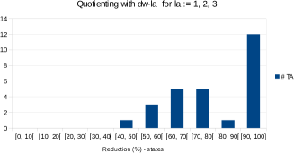
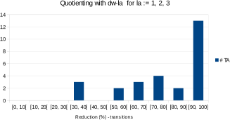
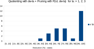
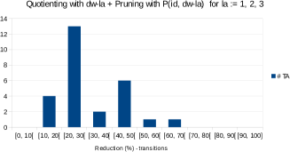
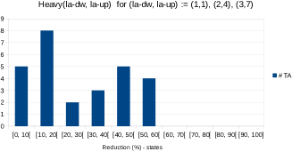
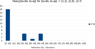
Figure 2: Reduction of 27 moderate-sized tree automata by methods RUQ (top row), RUQP (middle row), and Heavy (bottom row). A bar of height $h$ at an interval $[x,x+10[$ means that $h$ of the 27 automata were reduced to a size between $x\%$ and $(x+10)\%$ of their original size. The reductions in the numbers of states/transitions are shown on the left/right, respectively. On this set of automata, the methods Heavy(2,4) and Heavy(3,7) gave exactly the same results as Heavy(1,1).

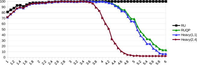
Figure 3: Reduction of Tabakov-Vardi random tree automata with $n=100,s=2$ and ${\it ad}=0.8$. The $x$-axis gives the transition density ${\it td}$, and the $y$-axis gives the average number of states after reduction with the various methods (smaller is better). Each data point is the average of 400 random automata. Note that Heavy(2,4) reduces much better than Heavy(1,1) for ${\it td}\geq 3.5$. Computing Heavy(x,y) for even higher $x,y$ is very slow on (some instances of) random automata.

The second set are 62 larger automata (586 states and 8865 transitions, on avg.) derived from regular model checking applications. Heavy(1,1), on avg., reduced the number of states and transitions to 4.2% and 0.7% of the original sizes. In contrast, RU did not perform any reduction in any case, RUQ, on avg., reduced the number of states and transitions to 75.2% and 74.8% of the original sizes and RUQP reduced the number of states and transitions to 75.2% and 15.8% of the original sizes; cf. Table 2 in App.0.D. The average computation times of Heavy(1,1), RUQP, RUQ and RU were, respectively, 2.7s, 2.1s, 0.2s and 0.02s.

The third set are 14,498 automata (57 states and 266 transitions on avg.) from the shape analysis tool Forester [22]. Heavy(1,1), on avg., reduced the number of states/transitions to 76.4% and 67.9% of the original, resp. RUQ and RUQP reduced the states and transitions only to 94% and 88%, resp. The average computation times of Heavy(1,1), RUQP, RUQ and RU were, respectively, 0.21s, 0.014s, 0.004s, and 0.0006s.

Due to the particular structure of the automata in these 3 sample sets, ${\it Heavy}(2,4)$ and ${\it Heavy}(3,7)$ had hardly any advantage over ${\it Heavy}(1,1)$. However, in general they can perform significantly better.

We also tested the algorithms on randomly generated tree automata, according to a generalization of the Tabakov-Vardi model of random word automata [23]. Given parameters $n,s$, ${\it td}$ (transition density) and ${\it ad}$ (acceptance density), it generates tree automata with $n$ states, $s$ symbols (each of rank 2), $n*{\it td}$ randomly assigned transitions for each symbol, and $n*{\it ad}$ randomly assigned leaf rules. Figure 3 shows the results of reducing automata of varying ${\it td}$ with different methods.

8 Summary and Conclusion

The tables in Figure 4 and Figure 5 summarize all our results on pruning and quotienting, respectively. Note that negative results propagate to larger relations and positive results propagate to smaller relations (i.e., GFP/GFQ is downward closed).

The experiments show that our Heavy(x,y) algorithm can significantly reduce the size of many classes of nondeterministic tree automata, and that it is sufficiently fast to handle instances with hundreds of states and thousands of transitions.

		$R_{\mathsf{d}}$
$R_{\mathsf{u}}\backslash R_{i}$		${\it id}$	$\sqsubset^{\mathsf{dw}}$	$\sqsubseteq^{\mathsf{dw}}$	$\subset^{\mathsf{dw}}$	$\subseteq^{\mathsf{dw}}$
${\it id}$	${\it id}$	$\--$	$\checkmark$	$\--$	$\checkmark$	$\--$
$\sqsubset^{\mathsf{up}}$	${\it id}$	$\checkmark$	$\checkmark$	$\checkmark$	$\checkmark$	$\checkmark$
	$\sqsubset^{\mathsf{dw}}$	$\times$	$\checkmark$	$\times$	$\times$	$\times$
	$\sqsubseteq^{\mathsf{dw}}$	$\times$	$\checkmark$	$\times$	$\times$	$\times$
	downup-rel.	$\checkmark$	$\checkmark$	$\checkmark$	$\checkmark$	$\checkmark$
	$\subset^{\mathsf{dw}}$	$\times$	$\times$	$\times$	$\times$	$\times$
	$\subseteq^{\mathsf{dw}}$	$\times$	$\times$	$\times$	$\times$	$\times$
$\sqsubseteq^{\mathsf{up}}$	${\it id}$	$\--$	$\checkmark$	$\--$	$\times$	$\--$
	$\sqsubset^{\mathsf{dw}}$	$\--$	$\checkmark$	$\--$	$\times$	$\--$
	$\sqsubseteq^{\mathsf{dw}}$	$\--$	$\checkmark$	$\--$	$\times$	$\--$
	$\subset^{\mathsf{dw}}$	$\--$	$\times$	$\--$	$\times$	$\--$
	$\subseteq^{\mathsf{dw}}$	$\--$	$\times$	$\--$	$\times$	$\--$
$\subset^{\mathsf{up}}$	${\it id}$	$\checkmark$	$\checkmark$	$\times$	$\times$	$\times$
	$\sqsubset^{\mathsf{dw}}$	$\times$	$\checkmark$	$\times$	$\times$	$\times$
	$\sqsubseteq^{\mathsf{dw}}$	$\times$	$\checkmark$	$\times$	$\times$	$\times$
	$\subset^{\mathsf{dw}}$	$\times$	$\times$	$\times$	$\times$	$\times$
	$\subseteq^{\mathsf{dw}}$	$\times$	$\times$	$\times$	$\times$	$\times$
$\subseteq^{\mathsf{up}}$	${\it id}$	$\--$	$\checkmark$	$\--$	$\times$	$\--$
	$\sqsubset^{\mathsf{dw}}$	$\--$	$\checkmark$	$\--$	$\times$	$\--$
	$\sqsubseteq^{\mathsf{dw}}$	$\--$	$\checkmark$	$\--$	$\times$	$\--$
	$\subset^{\mathsf{dw}}$	$\--$	$\times$	$\--$	$\times$	$\--$
	$\subseteq^{\mathsf{dw}}$	$\--$	$\times$	$\--$	$\times$	$\--$

Figure 4: GFP relations $P({R_{\mathsf{u}}(R_{i})},{R_{\mathsf{d}}})$ for tree automata. Relations which are GFP are marked with $\checkmark$, those which are not are marked with $\times$ and $\--$ is used to mark relations where the test does not apply due to them being reflexive (and therefore not asymmetric).

$R$
$\subseteq^{\mathsf{dw}}$		$\checkmark$
$\sqsubseteq^{\mathsf{dw}}$		$\checkmark$
$\sqsubseteq^{\mathsf{up}}$	${\it id}$	$\checkmark$
	$\sqsubset^{\mathsf{dw}}$	$\--$
	$\sqsubseteq^{\mathsf{dw}}$	$\times$
	$\subset^{\mathsf{dw}}$	$\--$
	$\subseteq^{\mathsf{dw}}$	$\times$
$\subseteq^{\mathsf{up}}$	${\it id}$	$\checkmark$
	$\sqsubset^{\mathsf{dw}}$	$\--$
	$\sqsubseteq^{\mathsf{dw}}$	$\times$
	$\subset^{\mathsf{dw}}$	$\--$
	$\subseteq^{\mathsf{dw}}$	$\times$

Figure 5: GFQ relations $R$ for tree automata. Relations which are GFQ are marked with $\checkmark$ and those which are not are marked with $\times$. The relations marked with $\--$ are not even reflexive in general (unless all transitions are linear; in this case we have a word automaton and these relations are the same as $\sqsubseteq^{\mathsf{up}}\!\!\!\;\!\!({\it id})$ and $\subseteq^{\mathsf{up}}\!\!\!\;\!({\it id})$, respectively).

Appendix 0.A Examples and Counterexamples for Tree Automata

(a) $A_{BU}=(\Sigma,Q,\delta_{BU},F=\{q_{1},q_{2}\})$.

(b) $A_{TD}=(\Sigma,Q,\delta_{TD},I=\{q_{1},q_{2}\})$.

(c) The trees accepted by $A_{BU}$ and $A_{TD}$.

Figure 6: Let $\Sigma$ be a ranked alphabet such that $\Sigma_{0}=\{d,e\}$, $\Sigma_{1}=\{c\}$ and $\Sigma_{2}=\{a,b\}$. Consider the BUTA $A_{BU}$ and the TDTA $A_{TD}$, where $Q=\{q_{1},\ldots,q_{5}\}$ and $\delta_{BU}=\{\langle\psi,e,q_{4}\rangle,\langle\psi,d,q_{5}\rangle,\langle q_{4},c,q_{3}\rangle,\langle q_{5},c,q_{3}\rangle,\langle q_{3}q_{4},a,q_{1}\rangle,\langle q_{3}q_{4},b,q_{2}\rangle\}$. $A_{TD}$ is obtained from $A_{BU}$ by reversing the transition rules in $\delta_{BU}$ and by swapping the roles of the accepting and the final states. The language accepted by the automata is $L=\{a(e,c(d)),a(e,c(e)),b(e,c(d)),b(e,c(e))\}$, as represented in c).

(a) Automaton $A_{1}$.

(b) Automaton $A_{2}$.

      

Figure 7: An example of two NFAs for which language inclusion holds but trace inclusion does not: the trace for $aa$ does not preserve acceptance in the second state in $A_{2}$.

In Figure 6, we present two examples of TA, a BUTA and a TDTA, where the second is obtained from the first. We draw the automata vertically, either bottom-up or top-down (depending on if it is a BUTA or a TDTA), to make the reading of an input tree more natural. The example in Figure 7 shows that language inclusion on NFAs (and, more generally, on TA) does not imply trace inclusion.

(a) Consider the macros $T_{1}$ and $T_{2}$. They are used in $b)$ to introduce new transitions and new states in the third level of the automaton as here defined. Note that each of the intermediate states in $T_{2}$ is smaller w.r.t $\subset^{\mathsf{dw}}$ than the intermediate state in $T_{1}$. Thus, when the first state in $T_{2}$ is smaller w.r.t $\sqsubset^{\mathsf{up}}\!\!\!\;\!(\sqsubset^{\mathsf{dw}})$ than the first state in $T_{1}$, each of the $d$-transitions in $T_{2}$ is a blue one w.r.t. the $d$-transition in $T_{1}$, which is red. Let us also consider the symbols $x$ and $y$ of rank $1$. We can extend a macro $T$ by adding transitions from the first state to some new state by $x$, by $y$ or by both and we denote these by $T_{x}$, $T_{y}$ or $T_{x+y}$, respectively.

(b) We consider $\Sigma_{0}=\{b,c\}$, $\Sigma_{1}=\{d,x,y,z\}$ and $\Sigma_{2}=\{a\}$. The dashed arrows represent transitions by $z$ from/to some new state. Each of the six initial states has an $a$-transition to one of the states from $7$ to $12$ on the left and one of the states from $7^{\prime}$ to $12^{\prime}$ on the right. Any state $n^{\prime}$ on the right side of the automaton does exactly the same downwardly as the state $n$ on the left side, and thus needs not be expanded in the figure. We abbreviate $\sqsubset^{\mathsf{up}}\!\!\!\;\!(\sqsubset^{\mathsf{dw}})$ to simply $\sqsubset^{\mathsf{up}}$ and $\sqsubseteq^{\mathsf{up}}\!\!\!\;\!\!(\sqsubset^{\mathsf{dw}})$ to $\sqsubseteq^{\mathsf{up}}$.

Figure 8: $P(\sqsubset^{\mathsf{up}}\!\!\!\;\!(\sqsubset^{\mathsf{dw}}),\subset^{\mathsf{dw}})$ is not GFP since the automaton presented in $b)$ cannot read the full binary tree of $a$’s with height $3$ without using a blue transition: a run starting in state $1$ encounters a blue transition from $7$, as illustrated in the figure; and since $7^{\prime}$ and $8^{\prime}$ do the same downwardly as $7$ and $8$, respectively, and since $7^{\prime}\sqsubset^{\mathsf{up}}8^{\prime}$, we have that there is a blue transition from $7^{\prime}$ as well, and so $2$ cannot be used either; since $17\sqsubset^{\mathsf{up}}18$ we have that, as explained in $a)$, there is a blue transition departing from $17$, thus a run starting at $3$ too cannot be used; and since $9$ is downwardly imitated by $9^{\prime}$, a run using this state finds a blue transition as well, and so $4$ is not safe; since $23\sqsubset^{\mathsf{up}}24$, a blue transition from $23$ exists and so $5$ cannot be used; finally, since $11$ is imitated by $11^{\prime}$, we have that a run using this state encounters a blue transition as well, and so $6$ too is not safe.

(a) Automaton $A$.

(b) Automaton $A/\equiv$.

Figure 9: $\equiv\,:=\,\sqsubseteq^{\mathsf{up}}\!\!\!\;\!\!(\sqsubseteq^{\mathsf{dw}}\!\!\cap\!\sqsupseteq^{\mathsf{dw}})\,\cap\sqsupseteq^{\mathsf{up}}\!\!(\sqsubseteq^{\mathsf{dw}}\!\!\cap\!\sqsupseteq^{\mathsf{dw}})$ is not GFQ. We are considering $\Sigma_{0}=\{a,b\}$ and $\Sigma_{2}=\{c\}$.
Computing all the necessary relations to quotient $A$ w.r.t. $\equiv$, we obtain $\sqsubseteq^{\mathsf{dw}}\,=\{(p,q),(r,s)\}=\sqsupseteq^{\mathsf{dw}}$ and $\sqsubseteq^{\mathsf{up}}\!\!\!\;\!\!(\sqsubseteq^{\mathsf{dw}}\!\!\cap\!\sqsupseteq^{\mathsf{dw}})=\{(q,r),(r,q)\}$. Thus $\equiv\;=\{(q,r),(r,q)\}$. Computing $A/\!\!\equiv$, we verify that $c(b,a)$ is now accepted by the automaton $A/\!\!\equiv$, while it was not in the language of $A$.

Appendix 0.B Proofs of Theorems

Theorem 4.1. For every strict partial order $R\,\subset\;\subseteq^{\mathsf{dw}}$, it holds that $P({\it id},R)$ is GFP.

Proof

Let $A^{\prime}=Prune(A,P({\it id},R))$. We show $L(A)\subseteq L(A^{\prime})$. If $t\in L(A)$ then there exists an accepting $t$-run $\pi$ in $A$. We show that there exists an accepting $t$-run $\pi^{\prime}$ in $A^{\prime}$.

We will call an accepting $t$-run $\tilde{\pi}$ in $A$ $i$-good if its first $i$ levels use only transitions of $A^{\prime}$. Formally, for every node $v\in dom(t)$ with $|v|<i$, $\langle\tilde{\pi}(v),t(v),\tilde{\pi}(v1)\ldots\tilde{\pi}(v\#(t(v)))\rangle$ is a transition of $A^{\prime}$. By induction on $i$, we will show that there exists an $i$-good accepting run on $t$ for every $i\leq h(t)$. In the base case $i=0$, the claim is trivially true since every accepting $t$-run of $A$, and particularly $\pi$, is $0$-good.

For the induction step, let us assume that the claim holds for some $i$. Since $A$ is finite, for every transition ${\it trans}$ there are only finitely many $A$-transitions ${\it trans}^{\prime}$ such that ${\it trans}\mathrel{P({\it id},R)}{\it trans}^{\prime}$. And since $P({\it id},R)$ is transitive and irreflexive, for each transition ${\it trans}$ in $A$ we have that either 1) ${\it trans}$ is maximal w.r.t. $P({\it id},R)$, or 2) there exists a $P({\it id},R)$-larger transition ${\it trans}^{\prime}$ which is maximal w.r.t. $P({\it id},R)$. Thus for every state $p$ and every symbol $\sigma$, there exists a transition by $\sigma$ departing from $p$ which is still in $A^{\prime}$.

Therefore, for every $i$-good accepting run $\pi^{i}$ on $t$, one easily obtains an accepting run $\pi^{i+1}$ which is $(i+1)$-good. In the first $i$ levels of $t$, $\pi^{i+1}$ is identical to $\pi^{i}$. In the $(i+1)$-th level of $t$, we have that for any transition ${\it trans}=\langle\pi^{i}(v),t(v),\pi^{i}(v1)\ldots\pi^{i}(v\#(t(v)))\rangle$, for $|v|=i$, either ${\it trans}$ is $P({\it id},R)$-maximal, and so we take $\pi^{i+1}(vj):=\pi^{i}(vj)$ for all $1\leq j\leq\#(t(v))$, or there exists a $P({\it id},R)$-larger transition ${\it trans}^{\prime}=\langle\pi^{i}(v),t(v),q_{1}\ldots q_{\#(t(v))}\rangle$ that is $P({\it id},R)$-maximal. By the definition of $P({\it id},R)$, we have that $(\pi^{i}(v1)\ldots\pi^{i}(v\#(t(v))))\mathrel{\hat{R}}(q_{1}\ldots q_{\#(t(v))})$, and we take $\pi^{i+1}(vj):=q_{j}$ for all $1\leq j\leq\#(t(v)))$. Since ${R}\subset{\subseteq^{\mathsf{dw}}}$, we have that for every $1\leq j\leq\#t(v)$, there is a run $\pi_{j}$ of $A$ such that $t_{v_{j}}\stackrel{{\scriptstyle\pi_{j}}}{{\Longrightarrow}}q_{j}$. The run $\pi^{i+1}$ on $t$ can hence be completed from every $q_{j}$ by the run $\pi_{j}$, which concludes the proof of the induction step.

Since a $h(t)$-good run is a run in $A^{\prime}$, the theorem is proven. ∎

Theorem 4.2. For every strict partial order $R\,\subset\;\subseteq^{\mathsf{up}}\!\!\!\;\!({\it id})$, it holds that $P(R,{\it id})$ is GFP.

Proof

Let $A^{\prime}=Prune(A,P(R,{\it id}))$. We will show that for every accepting run $\pi$ of $A$ on a tree $t$, there exists an accepting run $\hat{\pi}$ of $A^{\prime}$ on $t$.

Let us first define some auxiliary notation. For an accepting run $\pi$ of $A$ on a tree $t$, ${\it bad}(\pi)$ is the smallest subtree of $t$ which contains all nodes $v$ of $t$ where $\pi$ uses a transition of $A-A^{\prime}$, i.e., a transition which is not $P(R,{\it id})$-maximal (where by $\pi$ using a transition at node $v$ we mean that the symbol of the transition is $t(v)$, $\pi(v)$ is the left-hand side of the transition, and the vector of $\pi$-values of children of $v$ is its right-hand side). We will use the following auxiliary claim.

• For every accepting run $\pi$ of $A$ on a tree $t$ with $|{\it bad}(\pi)|>1$, there is an accepting run $\pi^{\prime}$ of $A$ on $t$ where ${\it bad}(\pi^{\prime})$ is a proper subtree of ${\it bad}(\pi)$.

To prove (C), assume that $v$ is a leaf of ${\it bad}(\pi)$ labeled by a transition $\langle{p},{\sigma},r_{1}\dotsc r_{n}\rangle$. By the definition of $P(R,{\it id})$ and by the minimality of ${\it bad}(\pi)$, there exists a $P(R,{\it id})$-maximal transition $\tau=\langle{p^{\prime}},{\sigma},r_{1}\dotsc r_{n}\rangle$ where $p\mathrel{\subset^{\mathsf{up}}\!\!\!\;\!({\it id})}p^{\prime}$. Since $p\mathrel{\subset^{\mathsf{up}}\!\!\!\;\!({\it id})}p^{\prime}$, it follows from the definition of $\subset^{\mathsf{up}}\!\!\!\;\!({\it id})$ that there exists a run $\pi^{\prime}$ of $A$ on $t$ that differs from $\pi$ only in labels of prefixes of $v$ (including $v$ itself) with $\pi^{\prime}(v)=p^{\prime}$. In other words, ${\it bad}(\pi^{\prime})$ differs from ${\it bad}(\pi)$ only in that it does not contain a certain subtree rooted by some ancestor of $v$. This subtree contains at least $v$ itself, since $\pi^{\prime}$ uses the $P(R,{\it id})$-maximal transition $\tau$ to label $v$. The tree ${\it bad}(\pi^{\prime})$ is hence a proper subtree of ${\it bad}(\pi)$, which concludes the proof of (C).

With (C) in hand, we are ready to prove the lemma. By finitely many applications of (C), starting from $\pi$, we obtain an accepting run $\hat{\pi}$ on $t$ where ${\it bad}(\hat{\pi})$ is empty (we only need finitely many applications since ${\it bad}(\pi)$ is a finite tree, and every application of (C) yields a run with a strictly smaller ${\it bad}$ subtree). Thus $\hat{\pi}$ is using only $P(R,{\it id})$-maximal transitions. Since $R$ and hence also $P(R,{\it id})$ are strict p.o., $A^{\prime}=Prune(A,P(R,{\it id}))$ contains all $P(R,{\it id})$-maximal transitions of $A$, which means that $\hat{\pi}$ is an accepting run of $A^{\prime}$ on $t$. ∎

Theorem 5.1. $\equiv^{\mathsf{dw}}$ is GFQ.

Proof

Let $A^{\prime}:=A/\!\!\equiv^{\mathsf{dw}}$. It is trivial that $L(A)\subseteq L(A^{\prime})$. For the reverse inclusion, we will show by induction on the height $i$ of $t$, that for any tree $t$, if $t\in D_{A^{\prime}}([q])$ for some $[q]\in[Q]$, then $t\in D_{A}(q)$. This guarantees $L(A^{\prime})\subseteq L(A)$ since if $[q]\in[I]$ then there is some $q^{\prime}\in I$ such that $q^{\prime}\equiv^{\mathsf{dw}}q$ and thus, by the definition of $\equiv^{\mathsf{dw}}$, $D_{A}(q^{\prime})=D_{A}(q)$.

In the base case $i=1$, $t$ is a leaf-node $\sigma$, for some $\sigma\in\Sigma$. By hypothesis, $t\in L(A^{\prime})$. So there exists $[q]\in[I]$ such that $t\Longrightarrow_{A^{\prime}}[q]$. So $\langle[q],\sigma,[\psi]\rangle\in\delta_{A^{\prime}}$. Since $[\psi]=\{\psi\}$, there exists $q^{\prime}\in[q]$ such that $\langle q^{\prime},\sigma,\psi\rangle\in\delta_{A}$. Since $[q]\in[I]$ there is some $q^{\prime\prime}\in I$ with $q^{\prime\prime}\equiv^{\mathsf{dw}}q\equiv^{\mathsf{dw}}q^{\prime}$. We have $t\in D_{A}(q^{\prime})=D_{A}(q^{\prime\prime})\subseteq L(A)$.

Let us now consider $i>1$. Let $\sigma$ be the root of the tree $t$, and let $t_{1},t_{2},\ldots,t_{n}$, where $n=\#(\sigma)$, denote each of the immediate subtrees of $t$. As we assume $t\in L(A^{\prime})$, there exists $[q]\in[I]$ such that $\langle[q],\sigma,[q_{1}][q_{2}]\ldots[q_{n}]\rangle\in\delta_{A^{\prime}}$, for some $[q_{1}],[q_{2}],\ldots,[q_{n}]\in[Q]$, such that $t_{i}\in D_{A^{\prime}}([q_{i}])$ for every $i$. By the definition of $\delta_{A^{\prime}}$, there are $q_{1}^{\prime}\in[q_{1}]$, $q_{2}^{\prime}\in[q_{2}]$, $\ldots$, $q_{n}^{\prime}\in[q_{n}]$ and $q^{\prime}\in[q]$, such that $\langle q^{\prime},\sigma,q_{1}^{\prime}q_{2}^{\prime}\ldots q_{n}^{\prime}\rangle\in\delta_{A}$. By induction hypothesis, we obtain $t_{i}\in D_{A}(q_{i})$ for every $i$. Since $q_{i}\equiv^{\mathsf{dw}}q_{i}^{\prime}$, it follows that $t_{i}\in D_{A}(q_{i}^{\prime})$ for every $i$ and thus $t\in D_{A}(q^{\prime})$. By $q\equiv^{\mathsf{dw}}q^{\prime}$, we conclude that $t\in D_{A}(q)$. ∎

Theorem 5.2. $\equiv^{\mathsf{up}}\!\!({\it id})$ is GFQ.

Proof

Let $\equiv\;:=\;\equiv^{\mathsf{up}}\!\!({\it id})$ and $A^{\prime}:=A/\!\equiv$. It is trivial that $L(A)\subseteq L(A^{\prime})$. For the reverse inclusion, we will show, by induction on the height $h$ of $t$, that for any tree $t$, if $t\in D_{A^{\prime}}([q])$ for some $[q]\in[Q]$, then $t\in D_{A}(q^{\prime})$ for some $q^{\prime}\in[q]$. This guarantees $L(A^{\prime})\subseteq L(A)$ since if $[q]\in[I]$ then, given that $\equiv$ preserves the initial states, $q^{\prime}\in I$.

In the base case $h=1$, the tree is a leaf-node $\sigma$, for some $\sigma\in\Sigma$. By hypothesis, $t\in L(A^{\prime})$. So there exists a $[q]\in[I]$ such that $t\Longrightarrow_{A^{\prime}}[q]$, and so $\langle[q],\sigma,[\psi]\rangle\in\delta_{A^{\prime}}$. By the definition of $\delta_{A^{\prime}}$ and since $[\psi]=\{\psi\}$ ($\equiv$ preserves acceptance), we have that there exists $q^{\prime}\in[q]$ such that $\langle q^{\prime},\sigma,\psi\rangle\in\delta_{A}$, and hence $t\Longrightarrow_{A}q^{\prime}$.

Let us now consider $h>1$. As we assume $t\in D_{A^{\prime}}([q])$, there must exist a transition $\langle[q],\sigma,[q_{1}]\ldots[q_{n}]\rangle\in\delta_{A^{\prime}}$, for $n=\#\sigma$ and some $[q_{1}],\ldots,[q_{n}]\in[Q]$ such that $t_{i}\in D_{A^{\prime}}([q_{i}])$ for every $i:0\leq i\leq n$, where the $t_{i}$s are the subtrees of $t$. We define the following auxiliary notion: a transition $\langle r,\sigma,r_{1}\ldots r_{n}\rangle$ of $A$ satisfying $r\in[q]$ and $\forall_{1\leq k\leq n}\ldotp r_{k}\in[q_{k}]$ is said to be $j$-good iff $\forall_{1\leq k\leq j}\ldotp t_{k}\in D_{A}(r_{k})$. We will use induction on $j$ to show that there is a $j$-good transition for any $j$, which implies that there is some state $\hat{r}\in[q]$ such that $t\in D_{A}(\hat{r})$.

The base case is $j=0$. By the definition of $\delta_{A^{\prime}}$ and the fact that $\langle[q],\sigma,[q_{1}]\ldots[q_{n}]\rangle\in\delta_{A^{\prime}}$, there exist $q_{1}^{\prime}\in[q_{1}]$, $\ldots$, $q_{n}^{\prime}\in[q_{n}]$ and $q^{\prime}\in[q]$ such that $\langle q^{\prime},\sigma,q_{1}^{\prime}\ldots q_{n}^{\prime}\rangle\in\delta_{A}$. This transition is trivially $0$-good.

To show the induction step, assume a transition $\mathit{trans}=\langle r,\sigma,r_{1}\ldots r_{n}\rangle$ that is $j$-good for $j\geq 0$, i.e., each $r_{i}$ is in $[q_{i}]$, $r\in[q]$, and $\forall_{1\leq i\leq j}\ldotp t_{i}\in D_{A}(r_{i})$. By the hypothesis of the outer induction on $h$, there is $r_{j+1}^{\prime}\in[r_{i+1}]$ such that $t_{j+1}\in D_{A}(r_{j+1}^{\prime})$. Notice that $r_{j+1}\equiv r^{\prime}_{j+1}$. Since $\mathit{trans}$ is a transition of $A$, there is a run $\pi^{\prime}$ of $A$ on a tree $t^{\prime}$ of the height 1 with the root symbol $\sigma$, and where $\pi^{\prime}(1)=r_{1},\ldots,\pi^{\prime}(n)=r_{n}$, and $\pi^{\prime}(\epsilon)=r$. Since $r_{j+1}\equiv r^{\prime}_{j+1}$, then, by the definition of $\equiv$, there is another $t^{\prime}$-run $\pi^{\prime\prime}$ such that $r^{\prime}=\pi^{\prime\prime}(\epsilon)\in[q]$, $\pi^{\prime\prime}(j+1)=r^{\prime}_{j+1}$, and $\forall_{i\neq j+1}\ldotp\pi^{\prime\prime}(i)=\pi^{\prime}(i)=r_{i}$. This run uses the transition $\mathit{trans}^{\prime}=\langle r^{\prime},\sigma,r_{1}\ldots r_{j}r^{\prime}_{j+1}r_{j+2}\ldots r_{n}\rangle$ in $A$. Since $\mathit{trans}$ is $j$-good and $t_{j+1}\in D_{A}(r^{\prime}_{j+1})$, we have that $\mathit{trans}^{\prime}$ is $(j+1)$-good. This concludes the inner induction on $j$, showing that there exists an $n$-good transition. Hence $t\in D_{A}(\hat{r})$ for some $\hat{r}\in[q]$, which proves the outer induction on the height $h$ of the tree, concluding the whole proof. ∎

Appendix 0.C Combined Preorder

In [4], the authors introduce the notion of combined preorder on an automaton and prove that its induced equivalence relation is GFQ. Let $\oplus$ be an operator defined as follows: given two preorders $H$ and $S$ over a set $Q$, for $x,y\in Q$, $x(H\oplus S)y$ iff $(i)\;x(H\circ S)y$ and $(ii)\;\forall z\in Q\,:\,yHz\,\Longrightarrow\,x(H\circ S)z$. Let $D$ be a downward simulation preorder and $U$ an upward simulation preorder induced by $D$. A combined preorder $W$ is defined as $W\,=\,D\,\oplus\,U^{-1}$. Since we have $D\,\oplus\,U^{-1}\;\subseteq\;D\,\circ\,U^{-1}$, for any states $x,y$ such that $x(D\,\oplus\,U^{-1})y$, there exists a state $z$, called a mediator, such that $x\,D\,z$ and $y\,U\,z$.

In the following, Lemmas 2 and 3 are used by Theorem 0.C.1 to show that any quotienting with the equivalence relation induced by a combined preorder is subsumed by Heavy(1,1). We use the maximal downward simulation $\sqsubseteq^{\mathsf{dw}}$ and the maximal upward simulation $\sqsubseteq^{\mathsf{up}}\!\!\!\;\!\!(\sqsubseteq^{\mathsf{dw}})$ in our proof. Note that any automaton $A$ which has been reduced with Heavy(1,1) satisfies $(1)\;A\,=\,A/(\sqsubseteq^{\mathsf{dw}}\!\cap\sqsupseteq^{\mathsf{dw}})\,=\,A/(\sqsubseteq^{\mathsf{up}}\!\!\!\;\!\!({\it id})\cap\sqsupseteq^{\mathsf{up}}\!\!({\it id}))$ due to the repeated quotienting, and $(2)\;A\,=\,Prune(A,P(\sqsubseteq^{\mathsf{up}}\!\!\!\;\!\!(\sqsubseteq^{\mathsf{dw}}),\sqsubset^{\mathsf{dw}}))$ due to the repeated pruning.

Lemma 2

Let $A$ be an automaton and $p$ and $q$ two states. If 1) $A\,=\,A/(\sqsubseteq^{\mathsf{dw}}\cap\sqsupseteq^{\mathsf{dw}})$ and 2) $A\,=\,Prune(A,P(\sqsubseteq^{\mathsf{up}}\!\!\!\;\!\!(\sqsubseteq^{\mathsf{dw}}),\sqsubset^{\mathsf{dw}}))$, then $(p\sqsubseteq^{\mathsf{dw}}q\land p(\sqsubseteq^{\mathsf{up}}\!\!\!\;\!\!(\sqsubseteq^{\mathsf{dw}}))q)\,\Longrightarrow\,p=q$.

Proof

From 1) it follows that $\sqsubseteq^{\mathsf{dw}}$ is antisymmetric, so if $p\sqsubseteq^{\mathsf{dw}}q$ then $p\sqsubset^{\mathsf{dw}}q\lor p=q$.

From $p(\sqsubseteq^{\mathsf{up}}\!\!\!\;\!\!(\sqsubseteq^{\mathsf{dw}}))q$, it follows that for any transition $\langle p^{\prime},\sigma,p_{1}\ldots p_{i}\ldots p_{\#(\sigma)}\rangle$ with $p_{i}=p$ there exists a transition $\langle q^{\prime},\sigma,q_{1}\ldots q_{i}\ldots q_{\#(\sigma)}\rangle$ with $q_{i}=q$ such that $p^{\prime}(\sqsubseteq^{\mathsf{up}}\!\!\!\;\!\!(\sqsubseteq^{\mathsf{dw}}))q^{\prime}$ and $p_{j}\sqsubseteq^{\mathsf{dw}}q_{j}$ for all $j:1\leq j\neq i\leq\#(\sigma)$. From $p=p_{i}\sqsubseteq^{\mathsf{dw}}q_{i}=q$, we have that $(p_{1}\ldots p\ldots p_{\#(\sigma)})\,\hat{\sqsubseteq}^{\mathsf{dw}}\,(q_{1}\ldots q\ldots q_{\#(\sigma)})$. From 2) it follows that there is no $k:1\leq k\leq\#(\sigma)$ such that $p_{k}\sqsubset^{\mathsf{dw}}q_{k}$. In particular, $\neg(p\sqsubset^{\mathsf{dw}}q)$. Thus we conclude that $p=q$. ∎

Lemma 3

Let $A$ be an automaton and $p$ and $q$ two states. If $A\,=\,A/(\sqsubseteq^{\mathsf{dw}}\cap\sqsupseteq^{\mathsf{dw}})$, then $(p\sqsubseteq^{\mathsf{up}}\!\!\!\;\!\!(\sqsubseteq^{\mathsf{dw}})q)\land(q\sqsubseteq^{\mathsf{up}}\!\!\!\;\!\!(\sqsubseteq^{\mathsf{dw}})p)\Longrightarrow(p\sqsubseteq^{\mathsf{up}}\!\!\!\;\!\!({\it id})q)\land(q\sqsubseteq^{\mathsf{up}}\!\!\!\;\!\!({\it id})p)$.

Proof

Since $A=A/(\sqsubseteq^{\mathsf{dw}}\cap\sqsupseteq^{\mathsf{dw}})$, for any two states $x$ and $y$ we have that $(x\sqsubseteq^{\mathsf{dw}}y)\,\Longrightarrow\,(x\sqsubset^{\mathsf{dw}}y\lor x=y)$.

Let $p$ and $q$ be states s.t. $p\sqsubseteq^{\mathsf{up}}\!\!\!\;\!\!(\sqsubseteq^{\mathsf{dw}})q$ and $q\sqsubseteq^{\mathsf{up}}\!\!\!\;\!\!(\sqsubseteq^{\mathsf{dw}})p$. By the definition of $\sqsubseteq^{\mathsf{up}}\!\!\!\;\!\!(\sqsubseteq^{\mathsf{dw}})$ it follows that for any transition $\langle p^{\prime},\sigma,p_{1}\ldots p_{i}\ldots p_{\#(\sigma)}\rangle$ with $p_{i}=p$ there exists a transition $\langle q^{\prime},\sigma,q_{1}\ldots q_{i}\ldots q_{\#(\sigma)}\rangle$ with $p^{\prime}\sqsubseteq^{\mathsf{up}}\!\!\!\;\!\!(\sqsubseteq^{\mathsf{dw}})q^{\prime}$ and $q_{i}=q$ such that for any $j:1\leq j\neq i\leq\#(\sigma)\cdot p_{j}\sqsubseteq^{\mathsf{dw}}q_{j}$, and vice-versa. We can thus construct an infinite sequence of matching transitions where, for every index $j\neq i$, the sequence of states at component $j$ is $\sqsubseteq^{\mathsf{dw}}$-increasing. However, since $A$ only has a finite number of states (and transitions), all these sequences must converge to some equivalence class w.r.t. $\sqsubseteq^{\mathsf{dw}}\cap\sqsupseteq^{\mathsf{dw}}$. Thus, for any transition $\langle p^{\prime},\sigma,p_{1}\ldots p_{i}\ldots p_{\#(\sigma)}\rangle$ with $p_{i}=p$ there exists a transition $\langle q^{\prime},\sigma,q_{1}\ldots q_{i}\ldots q_{\#(\sigma)}\rangle$ with $p^{\prime}\sqsubseteq^{\mathsf{up}}\!\!\!\;\!\!(\sqsubseteq^{\mathsf{dw}})q^{\prime}$ and $q_{i}=q$ such that for any $j:1\leq j\neq i\leq\#(\sigma)\cdot p_{j}\sqsubseteq^{\mathsf{dw}}q_{j}\wedge q_{j}\sqsubseteq^{\mathsf{dw}}p_{j}$, and vice-versa. However, since $A=A/(\sqsubseteq^{\mathsf{dw}}\cap\sqsupseteq^{\mathsf{dw}})$, we obtain that $p_{j}=q_{j}$ for $j:1\leq j\neq i\leq\#(\sigma)$. By repeating the same argument for the new pair of states $p^{\prime}$ and $q^{\prime}$, we get that $(p\sqsubseteq^{\mathsf{up}}\!\!\!\;\!\!({\it id})q)\land(q\sqsubseteq^{\mathsf{up}}\!\!\!\;\!\!({\it id})p)$ as required. Hence $(\sqsubseteq^{\mathsf{up}}\!\!\!\;\!\!(\sqsubseteq^{\mathsf{dw}})\cap(\sqsubseteq^{\mathsf{up}}\!\!\!\;\!\!(\sqsubseteq^{\mathsf{dw}}))^{-1})\;\subseteq\;(\sqsubseteq^{\mathsf{up}}\!\!\!\;\!\!({\it id})\cap(\sqsubseteq^{\mathsf{up}}\!\!\!\;\!\!({\it id}))^{-1})$. ∎

Theorem 0.C.1

Let $A$ be an automaton such that:
$(1)\;A\,=\,A/(\sqsubseteq^{\mathsf{dw}}\!\cap\sqsupseteq^{\mathsf{dw}})\,=\,A/(\sqsubseteq^{\mathsf{up}}\!\!\!\;\!\!({\it id})\cap\sqsupseteq^{\mathsf{up}}\!\!({\it id}))$, and
$(2)\;A\,=\,Prune(A,P(\sqsubseteq^{\mathsf{up}}\!\!\!\;\!\!(\sqsubseteq^{\mathsf{dw}}),\sqsubset^{\mathsf{dw}}))$.
Then $A=A/(W\cap W^{-1})$, where $W=\;\;\sqsubseteq^{\mathsf{dw}}\oplus(\sqsubseteq^{\mathsf{up}}\!\!\!\;\!\!(\sqsubseteq^{\mathsf{dw}}))^{-1}$.

Proof

We show that $(p\,W\,q)\land(q\,W\,p)\;\Longrightarrow\;p=q$, which implies $A\,=\,A/(W\cap W^{-1})$. Let $p\,W\,q$ and $q\,W\,p$, then by the definition of $W$, there exist mediators $r$ such that $p\sqsubseteq^{\mathsf{dw}}r$ and $q\sqsubseteq^{\mathsf{up}}\!\!\!\;\!\!(\sqsubseteq^{\mathsf{dw}})r$ and $s$ such that $q\sqsubseteq^{\mathsf{dw}}s$ and $p\sqsubseteq^{\mathsf{up}}\!\!\!\;\!\!(\sqsubseteq^{\mathsf{dw}})s$. By the definition of $W$, we have that $p\,(\sqsubseteq^{\mathsf{dw}}\circ(\sqsubseteq^{\mathsf{up}}\!\!\!\;\!\!(\sqsubseteq^{\mathsf{dw}}))^{-1})\,s$ and $q\,(\sqsubseteq^{\mathsf{dw}}\circ(\sqsubseteq^{\mathsf{up}}\!\!\!\;\!\!(\sqsubseteq^{\mathsf{dw}}))^{-1})\,r$. Thus, there exist mediators $t$ such that $p\sqsubseteq^{\mathsf{dw}}t$ and $s\sqsubseteq^{\mathsf{up}}\!\!\!\;\!\!(\sqsubseteq^{\mathsf{dw}})t$ and $u$ such that $q\sqsubseteq^{\mathsf{dw}}u$ and $r\sqsubseteq^{\mathsf{up}}\!\!\!\;\!\!(\sqsubseteq^{\mathsf{dw}})u$. By the transitivity of $\sqsubseteq^{\mathsf{up}}\!\!\!\;\!\!(\sqsubseteq^{\mathsf{dw}})$ we obtain that $p\sqsubseteq^{\mathsf{up}}\!\!\!\;\!\!(\sqsubseteq^{\mathsf{dw}})t$ and $q\sqsubseteq^{\mathsf{up}}\!\!\!\;\!\!(\sqsubseteq^{\mathsf{dw}})u$. From 1), 2) and Lemma 2 we obtain that $p=t$ and $q=u$. So we have $s\sqsubseteq^{\mathsf{up}}\!\!\!\;\!\!(\sqsubseteq^{\mathsf{dw}})p$ and $r\sqsubseteq^{\mathsf{up}}\!\!\!\;\!\!(\sqsubseteq^{\mathsf{dw}})q$. By Lemma 3 we obtain that $s\sqsubseteq^{\mathsf{up}}\!\!\!\;\!\!(id)p$ and $p\sqsubseteq^{\mathsf{up}}\!\!\!\;\!\!(id)s$, and $r\sqsubseteq^{\mathsf{up}}\!\!\!\;\!\!(id)q$ and $q\sqsubseteq^{\mathsf{up}}\!\!\!\;\!\!(id)r$. Thus by (1) we obtain that $p=s$ and $q=r$. Since $p\sqsubseteq^{\mathsf{dw}}r$ and $q\sqsubseteq^{\mathsf{dw}}s$, we conclude that $p=q$. ∎

Appendix 0.D More Data from the Experiments

TA name	$\#Q_{i}$	$\#Delta_{i}$	$\#Q_{f}$	$\#Delta_{f}$	Q reduction	Delta reduction	Time(s)
A0053	54	159	27	66	50	41.509434	0.015
A0054	55	241	28	93	50.909088	38.589211	0.024
A0055	56	182	27	73	48.214287	40.10989	0.017
A0056	57	230	24	55	42.105263	23.913044	0.017
A0057	58	245	24	58	41.379311	23.67347	0.020
A0058	59	257	25	65	42.372883	25.291828	0.019
A0059	60	263	24	59	40	22.43346	0.022
A0060	61	244	32	111	52.459015	45.491802	0.034
A0062	63	276	32	112	50.793655	40.579708	0.029
A0063	64	571	11	23	17.1875	4.028021	0.027
A0064	65	574	11	23	16.923077	4.006969	0.024
A0065	66	562	11	23	16.666668	4.092527	0.026
A0070	71	622	11	23	15.492958	3.697749	0.016
A0080	81	672	26	58	32.098763	8.630952	0.043
A0082	83	713	26	65	31.325302	9.116409	0.047
A0083	84	713	26	65	30.952381	9.116409	0.048
A0086	87	1402	26	112	29.885057	7.988588	0.103
A0087	88	1015	12	23	13.636364	2.26601	0.060
A0088	89	1027	12	23	13.483146	2.239532	0.063
A0089	90	1006	12	21	13.333334	2.087475	0.064
A0111	112	1790	11	42	9.821428	2.346369	0.139
A0117	118	2088	25	106	21.186441	5.076628	0.177
A0120	121	1367	12	21	9.917356	1.536211	0.068
A0126	127	1196	11	23	8.661418	1.923077	0.083
A0130	131	1504	11	23	8.396947	1.529255	0.044
A0172	173	1333	11	23	6.358381	1.725431	0.098
A0177	178	1781	26	58	14.606741	3.256597	0.085
Average	87.07	816.04	19.78	53.59	26.97	13.94	0.052

Table 1: Results on reducing the 27 moderate-sized tree automata (from libvata’s regular model checking examples) with our ${\it Heavy}(1,1)$ algorithm. The columns give the name of each automaton, $\#Q_{i}$: its original number of states, $\#Delta_{i}$: its original number of transitions, $\#Q_{f}$: the number of states after reduction, $\#Delta_{f}$: the number of transitions after reduction, the reduction ratio for states in percent $100*\#Q_{f}/\#Q_{i}$ (smaller is better), the reduction ratio for transitions in percent $100*\#Delta_{f}/\#Delta_{i}$ (smaller is better), and the computation time in seconds. Note that the reduction ratios for transitions are smaller than the ones for states, i.e., the automata get not only smaller but also sparser. Experiments run on Intel 3.20GHz i5-3470 CPU.

Tables 1 and  2 show the results of reducing two automata samples from libvata’s regular model checking examples with our ${\it Heavy}(1,1)$ algorithm. The first sample (Table 1) contains 27 automata of moderate size while the second one (Table 2) contains 62 larger automata. In both tables the columns give the name of each automaton, $\#Q_{i}$: original number of states, $\#Delta_{i}$: original number of transitions, $\#Q_{f}$: states after reduction, $\#Delta_{f}$: transitions after reduction, the reduction ratio for states in percent $100*\#Q_{f}/\#Q_{i}$ (smaller is better), the reduction ratio for transitions in percent $100*\#Delta_{f}/\#Delta_{i}$ (smaller is better), and the computation time in seconds. Note that the reduction ratios for transitions are smaller than the ones for states, i.e., the automata get sparser. The experiments were run on Intel 3.20GHz i5-3470 CPU.

TA name	$\#Q_{i}$	$\#Delta_{i}$	$\#Q_{f}$	$\#Delta_{f}$	Q reduction	Delta reduction	Time(s)
A246	247	2944	11	42	4.45	1.43	0.40
A301	302	4468	12	21	3.97	0.47	0.29
A310	311	3343	24	52	7.72	1.56	0.59
A312	313	3367	11	23	3.51	0.68	0.21
A315	316	3387	24	52	7.59	1.54	0.58
A320	321	3623	26	65	8.10	1.79	0.56
A321	322	3407	24	52	7.45	1.53	0.62
A322	323	3651	35	100	10.84	2.74	0.67
A323	324	6199	26	112	8.02	1.81	1.48
A328	329	3517	26	58	7.90	1.65	0.50
A329	330	5961	24	100	7.27	1.68	1.36
A334	335	3936	11	23	3.28	0.58	0.72
A335	336	3738	26	58	7.74	1.55	0.56
A339	340	5596	12	21	3.53	0.38	0.49
A348	349	3681	11	23	3.15	0.62	0.27
A354	355	3522	24	52	6.76	1.48	0.70
A355	356	3895	25	55	7.02	1.41	0.45
A369	370	4134	24	52	6.49	1.26	0.31
A387	388	4117	24	52	6.19	1.26	0.51
A390	391	5390	11	23	2.81	0.43	1.15
A400	401	5461	11	23	2.74	0.42	1.36
A447	448	7924	12	23	2.68	0.29	2.55
A483	484	5592	25	55	5.17	0.98	0.51
A487	488	4891	16	28	3.28	0.57	0.33
A488	489	8493	12	21	2.45	0.25	2.86
A489	490	8516	12	21	2.45	0.25	2.93
A491	492	8708	12	21	2.44	0.24	3.03
A493	494	7523	12	21	2.43	0.28	0.69
A494	495	8533	12	21	2.42	0.25	2.97
A496	497	8618	12	21	2.41	0.24	2.81
A498	499	8612	12	21	2.40	0.24	3.10
A501	502	8632	12	21	2.39	0.24	2.95
A532	533	8867	12	23	2.25	0.26	3.20
A569	570	8351	26	58	4.56	0.69	0.98
A589	590	9606	12	21	2.03	0.22	3.20
A620	621	9218	12	21	1.93	0.23	1.45
A646	647	6054	19	34	2.94	0.56	0.65
A667	668	8131	26	58	3.89	0.71	1.12
A670	671	11021	34	76	5.07	0.69	5.80
A673	674	11157	25	55	3.71	0.49	5.38
A676	677	11043	34	76	5.02	0.69	5.85
A678	679	11172	26	56	3.83	0.50	5.32
A679	680	11032	34	76	5.00	0.69	5.88
A689	690	11207	31	71	4.49	0.63	5.59
A691	692	11047	34	76	4.91	0.69	5.61
A692	693	11066	34	76	4.91	0.69	6.10
A693	694	11188	34	76	4.90	0.68	6.05
A694	695	11191	34	76	4.89	0.68	6.09
A695	696	11070	34	76	4.89	0.69	5.80
A700	701	11245	36	81	5.14	0.72	6.13
A701	702	11244	36	83	5.13	0.74	6.00
A703	704	11255	34	76	4.83	0.68	6.09
A723	724	9376	26	58	3.59	0.62	1.28
A728	729	11903	12	21	1.65	0.18	2.97
A756	757	8884	26	58	3.43	0.65	1.34
A837	838	13038	11	23	1.31	0.18	5.34
A881	882	15575	12	21	1.36	0.13	3.36
A980	981	21109	12	21	1.22	0.10	4.64
A1003	1004	21302	12	21	1.20	0.10	3.99
A1306	1307	19699	25	55	1.91	0.28	2.88
A1404	1405	18839	24	52	1.71	0.28	3.09
A2003	2004	30414	24	52	1.20	0.17	6.98
Average	586.21	8865.85	21.32	47.74	4.19	0.72	2.69

Table 2: Results on reducing the 62 larger automata (those not called moderate-sized) from libvata.

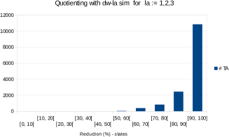
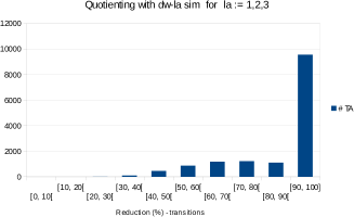
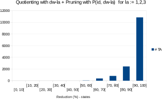
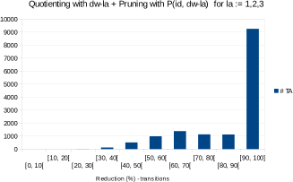
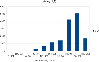
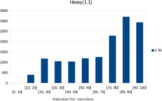
Figure 10: Reduction of 14498 tree automata from the Forester tool [22], by methods RUQ (top row), RUQP (middle row), and Heavy (bottom row). A bar of height $h$ at an interval $[x,x+10[$ means that $h$ of the 14498 automata were reduced to a size between $x\%$ and $(x+10)\%$ of their original size. The reductions in the numbers of states/transitions are shown on the left/right, respectively. Heavy(1,1) performed significantly better than RUQ and RUQP . Using lookaheads higher than 1 made hardly any difference in this sample set.

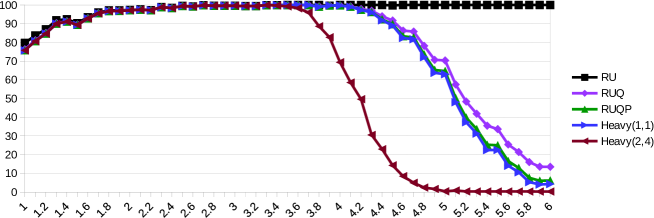
(a) This chart illustrates how the average number of transitions after reduction (in percent of the original number) with each method ($y$-axis) varied with the transition density $td$ of the sample ($x$-axis) being used (smaller is better). Note that Heavy(2,4) reduces much better than Heavy(1,1) for ${\it td}\geq 3.5$.

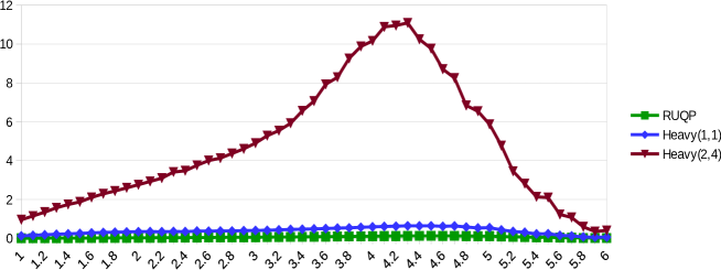
(b) This chart illustrates how the average time (in seconds) taken by each method ($y$-axis) varied with the transition density ${\it td}$ of the sample ($x$-axis) being used. Heavy(1,1) is significantly faster than Heavy(2,4), which has its time peak at ${\it td}=4.3$. RUQP is slightly faster than Heavy(1,1) and at ${\it td}=4.5$ it has its highest average value ($0.13$s).

Figure 11: Reduction of Tabakov-Vardi random tree automata with $n=100$, $s=2$ and ${\it ad}=0.8$. The top chart shows the average reduction in terms of number of transitions obtained with the various methods, while the bottom chart shows how long they took. Each data point in the charts is the average of 400 random automata.

References

- [1] P. A. Abdulla, A. Bouajjani, L. Holík, L. Kaati, and T. Vojnar. Computing simulations over tree automata. In TACAS, volume 4963 of LNCS, pages 93–108, 2008.
- [2] P. A. Abdulla, Y.-F. Chen, L. Holík, R. Mayr, and T. Vojnar. When simulation meets antichains. In J. Esparza and R. Majumdar, editors, TACAS, volume 6015 of Lecture Notes in Computer Science, pages 158–174. Springer, 2010.
- [3] P. A. Abdulla, L. Holík, B. Jonsson, O. Lengál, C. Q. Trinh, and T. Vojnar. Verification of heap manipulating programs with ordered data by extended forest automata. In D. V. Hung and M. Ogawa, editors, ATVA, volume 8172 of Lecture Notes in Computer Science, pages 224–239. Springer, 2013.
- [4] P. A. Abdulla, L. Holík, L. Kaati, and T. Vojnar. A uniform (bi-)simulation-based framework for reducing tree automata. Electr. Notes Theor. Comput. Sci., 251:27–48, 2009.
- [5] P. A. Abdulla, A. Legay, J. d’Orso, and A. Rezine. Simulation-based iteration of tree transducers. In Proc. TACAS ’05-11th Int. Conf. on Tools and Algorithms for the Construction and Analysis of Systems, volume 3440 of Lecture Notes in Computer Science, 2005.
- [6] P. A. Abdulla, A. Legay, J. d’Orso, and A. Rezine. Tree Regular Model Checking: A Simulation-Based Approach. J. Log. Algebr. Program., 69(1-2):93–121, 2006.
- [7] R. Almeida, L. Holík, and R. Mayr. HeavyMinOTAut. http://tinyurl.com/pm2b4qk, 2015.
- [8] D. Basin, N. Karlund, and A. Møller. Mona. http://www.brics.dk/mona, 2015.
- [9] F. Bonchi and D. Pous. Checking NFA equivalence with bisimulations up to congruence. In Principles of Programming Languages (POPL), Rome, Italy. ACM, 2013.
- [10] A. Bouajjani, P. Habermehl, L. Holík, T. Touili, and T. Vojnar. Antichain-based universality and inclusion testing over nondeterministic finite tree automata. In O. H. Ibarra and B. Ravikumar, editors, CIAA, volume 5148 of Lecture Notes in Computer Science, pages 57–67. Springer, 2008.
- [11] A. Bouajjani, P. Habermehl, A. Rogalewicz, and T. Vojnar. Abstract regular tree model checking of complex dynamic data structures. In SAS, volume 4134 of LNCS, pages 52–70, 2006.
- [12] L. Clemente and R. Mayr. Advanced automata minimization. In 40th Annual ACM SIGPLAN-SIGACT Symposium on Principles of Programming Languages, POPL, pages 63–74. ACM, 2013.
- [13] H. Comon, M. Dauchet, R. Gilleron, C. Löding, F. Jacquemard, D. Lugiez, S. Tison, and M. Tommasi. Tree automata techniques and applications. Available on: http://www.grappa.univ-lille3.fr/tata, 2008. release November, 18th 2008.
- [14] I. Durand. Autowrite. http://dept-info.labri.fr/~idurand/autowrite, 2015.
- [15] T. G. et al. Timbuk. http://www.irisa.fr/celtique/genet/timbuk/, 2015.
- [16] K. Etessami. A hierarchy of polynomial-time computable simulations for automata. In CONCUR, volume 2421 of LNCS, pages 131–144, 2002.
- [17] P. Habermehl, L. Holík, A. Rogalewicz, J. Simácek, and T. Vojnar. Forest automata for verification of heap manipulation. In Computer Aided Verification - 23rd International Conference, CAV 2011, Snowbird, UT, USA, July 14-20, 2011. Proceedings, pages 424–440, 2011.
- [18] L. Holík. Simulations and Antichains for Efficient Handling of Finite Automata. PhD thesis, Faculty of Information Technology of Brno University of Technology, 2011.
- [19] L. Holík, O. Lengál, A. Rogalewicz, J. Simácek, and T. Vojnar. Fully automated shape analysis based on forest automata. In CAV, volume 8044 of LNCS, pages 740–755, 2013.
- [20] L. Holík, O. Lengál, J. Simácek, and T. Vojnar. Efficient inclusion checking on explicit and semi-symbolic tree automata. In ATVA, volume 6996 of LNCS, pages 243–258, 2011.
- [21] O. Lengál, J. Simácek, and T. Vojnar. Libvata: highly optimised non-deterministic finite tree automata library. http://www.fit.vutbr.cz/research/groups/verifit/tools/libvata/, 2015.
- [22] O. Lengál, J. Simácek, T. Vojnar, P. Habermehl, L. Holík, and A. Rogalewicz. Forester: tool for verification of programs with pointers. http://www.fit.vutbr.cz/research/groups/verifit/tools/forester/, 2015.
- [23] D. Tabakov and M. Vardi. Model Checking Büchi Specifications. In LATA, volume Report 35/07. Research Group on Mathematical Linguistics, Universitat Rovira i Virgili, Tarragona, 2007.