Light-front $\phi^{4}_{1+1}$ theory
using a many-boson symmetric-polynomial basis

Abstract

We extend earlier work on fully symmetric polynomials for three-boson wave functions to arbitrarily many bosons and apply these to a light-front analysis of the low-mass eigenstates of $\phi^{4}$ theory in 1+1 dimensions. The basis-function approach allows the resolution in each Fock sector to be independently optimized, which can be more efficient than the preset discrete Fock states in DLCQ. We obtain an estimate of the critical coupling for symmetry breaking in the positive mass-squared case.

I Introduction

Our objective is to use newly developed multivariate polynomials GenSymPolys as a basis set for the computation of the odd and even-parity massive eigenstates of light-front $\phi_{1+1}^{4}$ theory RozowskyThorn ; Varyetal . The eigenvalue problem is solved in the form of a truncated Fock-state expansion, with each Fock wave function expanded in the polynomials. This allows separate tuning of the resolution in each Fock sector, which should be more efficient than a discrete light-cone quantization (DLCQ) PauliBrodsky ; DLCQreview calculation VaryHari . We can then study convergence with respect to the Fock-space truncation and compare results with those obtained with the light-front coupled-cluster (LFCC) method LFCC ; LFCCphi4 . We also estimate the value of the critical coupling for symmetry breaking.

The Lagrangian for two-dimensional $\phi^{4}$ theory is ${\cal L}=\frac{1}{2}(\partial_{\mu}\phi)^{2}-\frac{1}{2}\mu^{2}\phi^{2}-\frac{\lambda}{4!}\phi^{4}$, where $\mu$ is the mass of the boson and $\lambda$ is the coupling constant. The light-front Hamiltonian density is ${\cal H}=\frac{1}{2}\mu^{2}\phi^{2}+\frac{\lambda}{4!}\phi^{4}$. The mode expansion for the field at zero light-front time is

$$\phi=\int\frac{dp^{+}}{\sqrt{4\pi p^{+}}}\left\{a(p^{+})e^{-ip^{+}x^{-}/2}+a^{\dagger}(p^{+})e^{ip^{+}x^{-}/2}\right\},$$ (1)

with the modes quantized such that $[a(p^{+}),a^{\dagger}(p^{\prime+})]=\delta(p^{+}-p^{\prime+})$. The light-front Hamiltonian is ${\cal P}^{-}={\cal P}^{-}_{11}+{\cal P}^{-}_{13}+{\cal P}^{-}_{31}+{\cal P}^{-}_{22}$, with

$${\cal P}^{-}_{11} = \int dp^{+}\frac{\mu^{2}}{p^{+}}a^{\dagger}(p^{+})a(p^{+}),$$ (2)

$${\cal P}^{-}_{13} = \frac{\lambda}{6}\int\frac{dp_{1}^{+}dp_{2}^{+}dp_{3}^{+}}{4\pi\sqrt{p_{1}^{+}p_{2}^{+}p_{3}^{+}(p_{1}^{+}+p_{2}^{+}+p_{3}^{+})}}a^{\dagger}(p_{1}^{+}+p_{2}^{+}+p_{3}^{+})a(p_{1}^{+})a(p_{2}^{+})a(p_{3}^{+}),$$ (3)

$${\cal P}^{-}_{31} = \frac{\lambda}{6}\int\frac{dp_{1}^{+}dp_{2}^{+}dp_{3}^{+}}{4\pi\sqrt{p_{1}^{+}p_{2}^{+}p_{3}^{+}(p_{1}^{+}+p_{2}^{+}+p_{3}^{+})}}a^{\dagger}(p_{1}^{+})a^{\dagger}(p_{2}^{+})a^{\dagger}(p_{3}^{+})a(p_{1}^{+}+p_{2}^{+}+p_{3}^{+}),$$ (4)

$${\cal P}^{-}_{22} = \frac{\lambda}{4}\int\frac{dp_{1}^{+}dp_{2}^{+}}{4\pi\sqrt{p_{1}^{+}p_{2}^{+}}}\int\frac{dp_{1}^{\prime+}dp_{2}^{\prime+}}{\sqrt{p_{1}^{\prime+}p_{2}^{\prime+}}}\delta(p_{1}^{+}+p_{2}^{+}-p_{1}^{\prime+}-p_{2}^{\prime+})a^{\dagger}(p_{1}^{+})a^{\dagger}(p_{2}^{+})a(p_{1}^{\prime+})a(p_{2}^{\prime+}).$$ (5)

The eigenstate with momentum $P^{+}$ is expanded as

$$|\psi(P^{+})\rangle=\sum_{m}(P^{+})^{\frac{m-1}{2}}\int\prod_{i}^{m}dy_{i}\delta(1-\sum_{i}^{m}y_{i})\psi_{m}(y_{i})\frac{1}{\sqrt{m!}}\prod_{i=1}^{m}a^{\dagger}(y_{i}P^{+})|0\rangle.$$ (6)

The sum over $m$ is restricted to odd or even numbers. The Hamiltonian does not mix the two cases, and we solve for the lowest eigenstate in each case.

With use of the Fock-state expansion, the light-front Hamiltonian eigenvalue problem ${\cal P}^{-}|\psi(P)\rangle=\frac{M^{2}}{P}|\psi(P)\rangle$ becomes

$$\frac{m}{y_{1}}\psi_{m}(y_{i})+\frac{g}{4}\frac{m(m-1)}{\sqrt{y_{1}y_{2}}}\int\frac{dx_{1}dx_{2}}{\sqrt{x_{1}x_{2}}}\delta(y_{1}+y_{2}-x_{1}-x_{2})\psi_{m}(x_{1},x_{2},y_{3},\ldots,y_{m})$$ (7)

$$+\frac{g}{6}m\sqrt{(m+2)(m+1)}\int\frac{dx_{1}dx_{2}dx_{3}}{\sqrt{y_{1}x_{1}x_{2}x_{3}}}\delta(y_{1}-x_{1}-x_{2}-x_{3})\psi_{m+2}(x_{1},x_{2},x_{3},y_{2},\ldots,y_{m})$$

$$+\frac{g}{6}\frac{(m-2)\sqrt{m(m-1)}}{\sqrt{y_{1}y_{2}y_{3}(y_{1}+y_{2}+y_{3})}}\psi_{m-2}(y_{1}+y_{2}+y_{3},y_{4},\ldots,y_{m})=\frac{M^{2}}{\mu^{2}}\psi_{m}(y_{i}).$$

Here $g=\lambda/4\pi\mu^{2}$ is a dimensionless coupling. It is to this system of equations that we apply our basis-function expansion for each Fock-state wave function, to convert the coupled integral equations to a matrix eigenvalue problem.

II Solution of the integral equations

We solve this coupled system by first truncating the Fock-state expansion at some maximum number of constituents and then expanding each wave function in a basis of symmetric multivariate polynomials $P_{ni}^{(m)}$

$$\psi_{m}(y_{i})=\sqrt{\prod_{i}y_{i}}\sum_{ni}c_{ni}^{(m)}P_{ni}^{(m)}(y_{1},\ldots,y_{m}).$$ (8)

The $P_{ni}^{(m)}$ are of order $n$ and fully symmetric with respect to interchange of momenta GenSymPolys . The subscript $i$ differentiates the various possibilities at a given order $n$. For $m=2$ constituents there is only one possibility at each order, but for $m>2$ there can be more than one. For example, for three constituents there are two sixth-order polynomials, $P^{(3)}_{61}=(y_{1}y_{2}y_{3})^{2}$ and $P^{(3)}_{62}=(y_{1}y_{2}+y_{1}y_{3}+y_{2}y_{3})^{3}$.

The number of linearly independent polynomials of a given order is restricted by the constraint of momentum conservation, $\sum_{i}y_{i}=1$. For example, $P^{(3)}_{2}=y_{1}y_{2}+y_{1}y_{3}+y_{2}y_{3}$ is equivalent to $y_{1}^{2}+y_{2}^{2}+y_{3}^{2}$, up to a constant, when $y_{3}$ is replaced by $1-y_{1}-y_{2}$.

The linearly independent symmetric polynomials can be written as products of powers of simpler polynomials, in the form $P_{ni}^{(N)}=C_{2}^{n_{2}}C_{3}^{n_{3}}\cdots C_{N}^{n_{N}}$, with the powers restricted by $n=\sum_{j}jn_{j}$. Each different way of decomposing $n$ into a sum of integers greater than 1 yields a different polynomial. The $C_{m}$ are sums of simple monomials $\prod_{j}^{N}y_{j}^{m_{j}}$, where $m_{j}$ is 0 or 1 and $\sum_{j}^{N}m_{j}=m$. The sum over the monomials ranges over all possible choices for the $m_{j}$, making each $C_{m}$ fully symmetric.

As examples of the $C_{m}$, consider the general case of $N$ longitudinal momentum variables. Then $C_{2}$ is just $\sum_{j}^{N}\left(y_{j}\sum_{k>j}^{N}y_{k}\right)$; $C_{N-1}$ is $\sum_{j}^{N}\prod_{k\neq j}y_{k}$; and $C_{N}$ is $y_{1}y_{2}\cdots y_{N}$. In particular, for N=3, $C_{2}=y_{1}y_{2}+y_{1}y_{3}+y_{2}y_{3}$ and $C_{3}=y_{1}y_{2}y_{3}$. The first-order polynomial $C_{1}=\sum_{j}y_{j}$ does not appear because the momentum constraint reduces it to a constant.

Projection of the coupled system onto the basis functions yields the matrix equations

$$\sum_{n^{\prime}i^{\prime}}\left[T^{(m)}_{ni,n^{\prime}i^{\prime}}+gV^{(m,m)}_{ni,n^{\prime}i^{\prime}}\right]c^{(m)}_{n^{\prime}i^{\prime}}+g\sum_{n^{\prime}i^{\prime}}V^{(m,m+2)}_{ni,n^{\prime}i^{\prime}}c^{(m+1)}_{n^{\prime}i^{\prime}}+g\sum_{n^{\prime}i^{\prime}}V^{(m,m-2)}_{ni,n^{\prime}i^{\prime}}c^{(m-1)}_{n^{\prime}i^{\prime}}=\frac{M^{2}}{\mu^{2}}\sum_{n^{\prime}i^{\prime}}B^{(m)}_{ni,n^{\prime}i^{\prime}}c_{n^{\prime}i^{\prime}}^{(m)},$$ (9)

with $T^{(m)}$ the kinetic-energy matrix in the $m$th Fock sector

$$T^{(m)}_{ni,n^{\prime}i^{\prime}}=m\int\left(\prod_{j}dy_{j}\right)\delta(1-\sum_{j}y_{j})\left(\prod_{j=2}^{m}y_{j}\right)P_{ni}^{(m)}(y_{j})P_{n^{\prime}i^{\prime}}^{(m)}(y_{j}),$$ (10)

$B^{(m)}$ the basis-function overlap matrix

$$B^{(m)}_{ni,n^{\prime}i^{\prime}}=\int\left(\prod_{j}dy_{j}\right)\delta(1-\sum_{j}y_{j})\left(\prod_{j}^{m}y_{j}\right)P_{ni}^{(m)}(y_{j})P_{n^{\prime}i^{\prime}}^{(m)}(y_{j}),$$ (11)

and $V^{(m,m^{\prime})}$ the potential-energy matrices

$$V^{(m,m)}_{ni,n^{\prime}i^{\prime}} = \frac{g}{4}m(m-1)\int\left(\prod_{j}dy_{j}\right)\delta(1-\sum_{j}y_{j}$$

$$\times\int dx_{1}dx_{2}\delta(y_{1}+y_{2}-x_{1}-x_{2})\left(\prod_{j=3}^{m}y_{j}\right)P_{ni}^{(m)}(y_{j})P_{n^{\prime}i^{\prime}}^{(m)}(x_{1},x_{2},y_{3},\ldots,y_{m}),$$

$$V^{(m,m+2)}_{ni,n^{\prime}i^{\prime}} = \frac{g}{6}m\sqrt{(m+2)(m+1)}\int\left(\prod_{j}dy_{j}\right)\delta(1-\sum_{j}y_{j})$$

$$\times\int dx_{1}dx_{2}dx_{3}\delta(y_{1}-x_{1}-x_{2}-x_{3})\left(\prod_{j=2}^{m}y_{j}\right)P_{ni}^{(m)}(y_{j})P_{n^{\prime}i^{\prime}}^{(m+2)}(x_{1},x_{2},x_{3},y_{2},\ldots,y_{m}),$$

$$V^{(m,m-2)}_{ni,n^{\prime}i^{\prime}} = \frac{g}{6}(m-2)\sqrt{m(m-1)}\int\left(\prod_{j}dy_{j}\right)\delta(1-\sum_{j}y_{j})$$

$$\times\left(\prod_{j=4}^{m}y_{j}\right)P_{ni}^{(m)}(y_{j})P_{n^{\prime}i^{\prime}}^{(m-2)}(y_{1}+y_{2}+y_{3},y_{4},\ldots,y_{m}).$$

All of the integrals can be done analytically in terms of a generalized beta function.

We now have a generalized eigenvalue problem of the form $H\vec{c}=(M^{2}/\mu^{2})B\vec{c}$. A standard approach would be to factorize $B$ and convert the original problem to an ordinary eigenvalue problem. However, factorization can fail in practice due to round-off errors in the implicit orthogonalization of the basis. Round-off errors also plague an explicit orthogonalization. A reliable factorization is a singular-value decomposition $B=UDU^{T}$, where the columns of the matrix $U$ are the eigenvectors of $B$ and $D$ is a diagonal matrix of the eigenvalues of $B$. We then solve $H^{\prime}\vec{c}^{\,\prime}=(M^{2}/\mu^{2})\vec{c}^{\,\prime}$, with $H^{\prime}=D^{-1/2}U^{T}HUD^{-1/2}$ and $\vec{c}^{\,\prime}=D^{1/2}U^{T}\vec{c}$. Results for particular truncations of the polynomial basis are extrapolated to an infinite basis size in each Fock sector.

III Results

The results for the odd and even cases are shown in Fig. 1, where $M^{2}$ is plotted in units of the bare mass squared $\mu^{2}$ for a range of dimensionless coupling strengths $g$. The convergence with respect to Fock sector truncation is easily seen to be rapid, with the last two truncations yielding identical results to within errors in each case. We also compare the lowest order LFCC results LFCCphi4 for the odd case and find that these are quite consistent with the converged Fock-space calculation, even though the LFCC calculation involves only a three-body function.

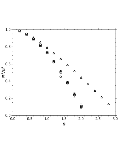
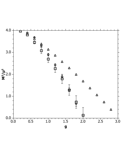
(a)	(b)

Figure 1: Mass squared vs coupling strength for an (a) odd and (b) even number of constituents. The different Fock-space truncations in (a) are the three-body (triangles), five-body (squares), and seven-body (diamonds) Fock sectors. Results for the LFCC method (circles) are also included. In (b) the different truncations are the four-body (triangles), six-body (squares), and eight-body (diamonds) Fock sectors. Error bars are determined by the fits to extrapolation in the polynomial basis size.

For both the odd and even cases, the mass crosses zero at a finite value of the coupling, with the massive eigenstate becoming degenerate with the Fock vacuum. We interpret this as the appearance of symmetry breaking and extract a value of the critical coupling, with use of the results as plotted in Fig. 2. The odd and even cases cross zero at nearly the same value. As a check, we plot points for four times the $M^{2}$ values in the odd case; in an exact calculation these should coincide with the even values, and here they are close, consistent with the errors in each. From the figure we estimate the critical coupling to be $g_{c}=2.1\pm 0.05$.

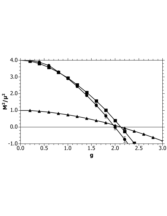
Figure 2: Mass squared vs coupling strength, as used to estimate the critical coupling. The odd (triangles) and even (circles) cases are represented by the seven-body and eight-body truncations, respectively. Points at twice the mass of the odd case (squares) are also plotted.

Comparison with other calculations of the critical coupling, as summarized in Table 1, can be readily made. However, the values compiled by Rychkov and Vitale RychkovVitale are normalized in a slightly different manner; the translation from our $g$ to theirs is $\bar{g}=\frac{\pi}{6}g$. Clearly there is a systematic difference between equal-time and light-front values. However, this is consistent with the expectation that the renormalization of the mass $\mu$ is different in the two quantizations Burkardt . Calculations to evaluate this difference quantitatively are underway.

Table 1: Comparison of values for the critical coupling, with $\bar{g}=\frac{\pi}{6}g$, as compiled in Ref. RychkovVitale . The first two use light-front quantization; the remainder use equal-time quantization.

Method	$\bar{g}_{c}$	Reported by
LF symmetric polynomials	$1.1\pm 0.03$	this talk
DLCQ	1.38	Harindranath & Vary VaryHari
Quasi-sparse eigenvector	2.5	Lee & Salwen LeeSalwen
Density matrix renormalization group	2.4954(4)	Sugihara Sugihara
Lattice Monte Carlo	2.70$\left\{\begin{array}[]{l}+0.025\\ -0.013\end{array}\right.$	Schaich & Loinaz SchaichLoinaz
Uniform matrix product	2.766(5)	Milsted et al. Milsted
Renormalized Hamiltonian truncation	2.97(14)	Rychkov & Vitale RychkovVitale

IV Summary

We have developed a high-order method for (1+1)-dimensional light-front theories that is distinct from DLCQ. The method employs function expansions in terms of fully symmetric multivariate polynomials that respect the constraint of momentum conservation. It allows separate tuning of resolutions in each Fock sector, and could be combined with transverse discretization or basis functions for applications to (3+1)-dimensional theories.

The method has been applied to $\phi^{4}_{1+1}$ theory, to compute the lowest mass eigenvalues and to extract an estimate of critical coupling for the positive $\mu^{2}$ case. We have identified a systematic difference with equal-time quantization which can be associated with the difference in mass renormalizations of the two quantizations Burkardt . We have also compared these converged high-order Fock space truncations with the lowest-order LFCC calculation LFCCphi4 and found good agreement, which implies that the LFCC method shows promise for rapid convergence.

References

• (1) Chabysheva SS, Hiller JR (2014) Basis of symmetric polynomials for many-boson light-front wave functions. Phys. Rev. E 90: 063310;
Chabysheva SS, Elliott B, Hiller JR (2013) Symmetric multivariate polynomials as a basis for three-boson light-front wave functions. Phys. Rev. E 88: 063307
• (2) Rozowsky JS, Thorn CB (2000) Spontaneous symmetry breaking at infinite momentum without $P^{+}$ zero modes. Phys. Rev. Lett. 85: 1614-1617
• (3) Kim VT, Pivovarov GB, Vary JP (2004) Phase transition in light-front $\phi_{1+1}^{4}$. Phys. Rev.  D 69: 085008;
Chakrabarti D, Harindranath A, Martinovic L, Vary JP (2004) Kinks in discrete light cone quantization. Phys. Lett. B 582: 196-202;
Chakrabarti D, Harindranath A, Martinovic L, Pivovarov GB, Vary JP (2005) Ab initio results for the broken phase of scalar light front field theory. Phys. Lett. B 617: 92-98;
Chakrabarti D, Harindranath A, Vary JP (2005) Transition in the spectrum of the topological sector of $\phi^{4}_{2}$ theory at strong coupling. Phys. Rev. D 71: 125012;
Martinovic L (2008) Spontaneous symmetry breaking in light front field theory. Phys. Rev. D 78: 105009
• (4) Pauli H-C, Brodsky SJ (1985) Solving field theory in one space and one time dimension. Phys. Rev. D 32: 1993-2000;
Discretized light-cone quantization: Solution to a field theory in one space and one time dimension. Phys. Rev. D 32: 2001-2013
• (5) Brodsky SJ, Pauli H-C, Pinsky SS (1998) Quantum chromodynamics and other field theories on the light cone. Phys. Rep. 301: 299-486
• (6) Harindranath A, Vary JP (1987) Solving two-dimensional $\phi^{4}$ theory by discretized light-front quantization. Phys. Rev. D 36: 1141-1147
• (7) Chabysheva SS, Hiller, JR (2012) A light-front coupled-cluster method for the nonperturbative solution of quantum field theories. Phys. Lett. B 711: 417-422
• (8) Elliott B, Chabysheva SS, Hiller JR (2014) Application of the light-front coupled-cluster method to $\phi^{4}$ theory in two dimensions. Phys. Rev. D 90: 056003
• (9) Rychkov S, Vitale LG (2015) Hamiltonian truncation study of the $\phi^{4}$ theory in two dimensions. Phys. Rev. D 91: 085011
• (10) Burkardt M (1993) Light-front quantization of the sine-Gordon model. Phys. Rev. D 47: 4628-4633
• (11) Lee D, Salwen N (2001) The diagonalization of quantum field hamiltonians. Phys. Lett. B 503: 223-
• (12) Sugihara T (2004) Density matrix renormalization group in a two-dimensional lambda $\phi^{4}$ Hamiltonian lattice model. J. High Energy Phys. 05(2004): 007
• (13) Schaich D, Loinaz W (2009) An improved lattice measurement of the critical coupling in $\phi^{4}_{2}$ theory. Phys. Rev. D 79: 056008
• (14) Milsted A, Haegeman J, Osborne TJ (2013) Matrix product states and variational methods applied to critical quantum field theory. Phys. Rev. D 88: 085030