A geometrothermodynamic approach to ideal quantum gases and Bose-Einstein condensates

Abstract

We analyze in the context of geometrothermodynamics the behavior of ideal quantum gases which satisfy either the Fermi statistics or the Bose statistics. Although the corresponding Hamiltonian does not contain a potential, indicating the lack of classical thermodynamic interaction, we show that the curvature of the equilibrium space is non-zero, and can be interpreted as a measure of the effective quantum interaction between the gas particles. In the limiting case of a classical Boltzmann gas, we show that the equilibrium space becomes flat, as expected from the physical viewpoint. In addition, we derive a thermodynamic fundamental equation for the Bose-Einstein condensation and, using the Ehrenfest scheme, we show that it can be considered as a first-order phase transition which in the equilibrium space corresponds to a curvature singularity. This result indicates that the curvature of the equilibrium space can be used to measure the thermodynamic interaction in classical and quantum systems.

I Introduction

In 1915, Einstein formulated the final version of the gravitational field equations that were based upon the astonishing principle “gravitational interaction = curvature”. In this case, the curvature is the Riemannian curvature of the 4-dimensional spacetime. This principle has been generalized to include all the four interactions known in nature (see, for instance, Ref. frankel ). Indeed, Yang and Mills ym53 demonstrated in 1953 that the field strength (Faraday tensor) of the electromagnetic field can be interpreted as the curvature of a principal fiber bundle, with the Minkowski spacetime as the base manifold and the symmetry group $U(1)$ as the standard fiber. Today, it is well known frankel that the weak interaction and the strong interaction can be described by the curvature of a principal fiber bundle with standard fiber $SU(2)$ and $SU(3)$, respectively. In this sense, we can say that all the field theories have a well-formulated geometric description.

On the other hand, Riemannian geometry has been also applied in statistical physics and thermodynamics. To this end, one can consider the equilibrium states of the thermodynamic system as points of an abstract space (equilibrium space). Then, one of the goals of applying differential geometry in thermodynamics is to interpret the curvature of the equilibrium space as a measure of the thermodynamic interaction. In 1945, Rao rao45 introduced in the equilibrium space a Riemannian metric whose components in local coordinates coincide with the Fisher information matrix. Rao’s original work has been followed up and extended by a large number of authors (see, e.g., amari85 for a review). On the other hand, Riemannian geometry in the space of equilibrium states was introduced by Weinhold wei75 and Ruppeiner rup79 ; rup95 , who defined metric structures as the Hessian of the internal energy and the entropy, respectively.

Geometrothermodynamics (GTD) quev07 was proposed recently to take into account the invariance of classical thermodynamics under a change of thermodynamic potential callen , a property which is not shared by Hessian metrics. In contrast to other geometric approaches, GTD resembles the approach of field theories in the sense that the symmetry of the theory plays a fundamental role in its geometric description. Since different thermodynamic potentials are related by means of Legendre transformations arnold , the formalism of GTD makes use of the Riemannian contact structure of the thermodynamic phase space her73 to handle Legendre invariance correctly from a mathematical point of view. The equilibrium space can then be considered as a particular subspace of the phase space. As a result, the formalism of GTD uses as starting point a Legendre invariant metric of the phase space which induces a metric in the equilibrium space whose curvature should describe the thermodynamic interaction. In the case of a classical ideal gas, for which the corresponding Hamiltonian does not contain a potential term that could represent any interaction between the gas particles huang , no thermodynamic interaction is present and one would expect that the corresponding equilibrium space be flat. In fact, this physical condition has been used to fix the metric of the phase space quev07 . The flat equilibrium manifold of a classical ideal gas has been investigated in detail recently qsv15 . In particular, it was found that there exists a deep relationship between geodesics and quasi-static processes which gives rise to a relativistic like structure of the equilibrium manifold.

In the case of ideal quantum gases, the Hamiltonian also does not contain a potential term and the gas particles are assumed to have no interaction between them huang ; greiner . This means that from the point of view of the Hamiltonian approach a quantum gas is a system without thermodynamic interaction. One would then expect that the corresponding equilibrium manifold is also flat due to the lack of interaction. Nevertheless, we know that the physical properties of ideal quantum gases are different from those of a classical ideal gas. The question arises whether our geometric approach is able to take into account those physical differences in a consistent manner. The main purpose of the present work is to show that in the framework of GTD the ideal quantum gases are represented by non-flat equilibrium manifolds, taking into account the quantum nature of the gas particles. Moreover, we analyze the limiting case of Bose-Einstein condensation and show that it can be interpreted in the Ehrenfest scheme and in GTD as a first-order phase transition.

This paper is organized as follows. In Sec. II, we review the main aspects of GTD which are necessary in order to take into account the Legendre invariance of classical thermodynamics. In Sec. III, we derive the fundamental equation of quantum ideal gases which is necessary to carry out the geometrothermodynamic approach. In Sec. IV, we investigate the thermodynamic and geometrothermodynamic properties of Bose-Einstein condensates. Finally, in Sec. V, we discuss our results.

II A review of geometrothermodynamics

The starting point of the GTD formalism is the thermodynamic phase space ${\cal T}$ which is constructed as follows. A thermodynamic system with $n$ degrees of freedom is described by a set of $n$ extensive variables, $E^{a}$, $n$ intensive variables, $I^{a}$ $(a=1,...,n)$, and a thermodynamic potential, $\Phi$. Let us consider $Z^{A}=\{\Phi,E^{a},I^{a}\}$ as the coordinates of the $(2n+1)-$dimensional space ${\cal T}$. A thermodynamic system is usually described by a fundamental equation $\Phi=\Phi(E^{a})$. In GTD, the specification of a particular system corresponds to an embedding $\varphi$ of an $n$-dimensional manifold $\mathcal{E}$ into the phase space $\mathcal{T}$ given by

$$\varphi:\mathcal{E}\longrightarrow\mathcal{T},$$ (1)

or, in coordinates,

$$\varphi:\{E^{a}\}\longrightarrow\{\Phi(E^{a}),E^{a},I^{b}(E^{a}),\}\ .$$ (2)

The space $\mathcal{T}$ is endowed with a family of tangent hyperplanes (contact structure) defined by the fundamental 1-form $\Theta$ that satisfies the non-integrability condition her73

$$\Theta\wedge(d\Theta)^{n}\neq 0\ .$$ (3)

The phase space is necessary in order to treat the Legendre transformations of classical thermodynamics as a change of coordinates. Formally, a Legendre transformation is defined as arnold

$$\{Z^{A}\}\rightarrow\{\tilde{Z}^{A}\}=\{\tilde{\Phi},\tilde{E}^{a},\tilde{I}^{a}\}$$ (4)

$$\Phi=\tilde{\Phi}-\delta_{kl}\tilde{E}^{k}\tilde{I}^{l}\,,\quad E^{i}=-\tilde{I}^{i}\,,E^{j}=\tilde{E}^{j}\,,\ I^{i}=\tilde{E}^{i}\,,\ I^{j}=\tilde{I}^{j}\ ,$$ (5)

where $i\cup j$ is any disjoint decomposition of the set of indices $\{1,\ldots,n\}$, and $k,l=1,\ldots,i$.

According to the Darboux theorem her73 , if we use the coordinates $\{Z^{A}\}$ the fundamental 1-form $\Theta$ can be written as

$$\Theta=d\Phi-I_{a}dE^{a}\ ,\quad I_{a}=\delta_{ab}I^{b}\ ,$$ (6)

where we assume Einstein’s summation convention for repeated indices. If we apply the Legendre transformation to $\Theta$, the new 1-form $\tilde{\Theta}$ in coordinates $\{\tilde{Z}^{A}\}$ reads

$$\tilde{\Theta}=d\tilde{\Phi}-\tilde{I}_{a}d\tilde{E}^{a}\ .$$ (7)

This proves that the contact 1-form $\Theta$ is invariant with respect to Legendre transformations.

On other hand, the space $\mathcal{E}$ is determined through the embedding (1), which is equivalent to specifying the fundamental equation of the system $\Phi(E^{a})$. To complete the GTD scheme, it is necessary to incorporate the relations of standard equilibrium thermodynamics into the definition of the space ${\cal E}$. This can be done by demanding that the embedding (1) satisfies the condition

$$\varphi^{*}(\Theta)=0\ ,$$ (8)

where $\varphi^{*}$ is the pullback of $\varphi$. In coordinates, it takes the form

$$\varphi^{*}(\Theta)=\varphi^{*}\left(d\Phi-I_{a}dE^{a}\right)=\left(\frac{\partial\Phi}{\partial E^{a}}-I_{a}\right)dE^{a}=0.$$ (9)

Then, it follows that

$$\Phi=\Phi(E^{a})\quad\text{and}\quad\frac{\partial\Phi}{\partial E^{a}}=I_{a}\ .$$ (10)

Equations (9) and (10) constitute the standard Gibbs relations of equilibrium thermodynamics in $\mathcal{E}$, namely,

$$d\Phi=I_{a}dE^{a}\ ,$$ (11)

which is the first law of thermodynamics. The manifold $\mathcal{E}$ is called the equilibrium space.

In GTD, the phase space is equipped with a metric $G$ which must be invariant with respect to Legendre transformations. Consequently, the triad $(\mathcal{T},\Theta,G)$ becomes a Riemannian contact manifold that is also Legendre invariant. So far, the most general metric invariant under total and partial Legendre transformations that has been found in GTD can be expressed as vqs09

$$G=\Theta^{2}+\Lambda\left(Z^{A}\right)\left(E_{a}I_{a}\right)^{2k+1}dE^{a}dI^{a}\ ,\quad I_{a}=\delta_{ab}I^{b}\ ,$$ (12)

where $\Lambda(Z^{A})$ is an arbitrary Legendre invariant function of the coordinates $Z^{A}$, and $k$ is an integer. Here we introduce the convention that the summation must be performed over all repeated covariant and contravariant indices. The arbitrariness contained in the function $\Lambda(Z^{A})$ and in the integer $k$ can be fixed by introducing the new coordinates (no summation over repeated indices)

$$dX^{a}=\sqrt{\Lambda}E_{a}^{2k+1}dE^{a}\ ,\qquad dY^{a}=\sqrt{\Lambda}I_{a}^{2k+1}dI^{a}$$ (13)

so that the metric (12) becomes

$$G=\Theta^{2}+\delta_{ab}dX^{a}dY^{b}\ .$$ (14)

All the further calculations could be performed in coordinates $(\Phi,X^{a},Y^{a})$, absorbing so the arbitrariness contained in (12). However, for the treatment of specific thermodynamic systems it is convenient to use the coordinates $(\Phi,E^{a},I^{a})$. Then, for concreteness let us consider the case $\Lambda=1$ and $k=0$ to obtain

$$G=\Theta^{2}+\left(E_{a}I_{a}\right)dE^{a}dI^{a}\ .$$ (15)

The corresponding induced thermodynamic metric in the space of equilibrium states is given by

$$g=\varphi^{*}(G)=E_{a}\frac{\partial\Phi}{\partial E^{a}}\delta^{ab}\frac{\partial^{2}\Phi}{\partial E^{b}\partial E^{c}}\ dE^{a}dE^{c}\ .$$ (16)

In the case of a system with two degrees of freedom, $n=2$, the above metric can be written explicitly as

$$g=E^{1}\Phi_{,1}\Phi_{,11}(dE^{1})^{2}+(E^{1}\Phi_{,1}+E^{2}\Phi_{,2})\Phi_{,12}dE^{1}dE^{2}+E^{2}\Phi_{,2}\Phi_{,22}(dE^{2})^{2}\ ,$$ (17)

where $\Phi_{,1}=\frac{\partial\Phi}{\partial E^{1}}$, etc. Notice that to calculate the explicit components of this metric, it is necessary to specify only the fundamental equation $\Phi=\Phi(E^{1},E^{2})$. Thus, all the geometric properties of the equilibrium space are determined by the fundamental equation. This is similar to the situation in classical thermodynamics where the fundamental equation is used to determine all the thermodynamic properties and equations of state of the system.

It is worth noticing that the coordinate sets $X^{a}$ and $Y^{a}$ as introduced above in Eq.(14) are specially adapted to investigate the physical significance of the equilibrium manifold metric. Indeed, one can show that this coordinate change can be understood as a diffeomorphism of the form $(\Phi,E^{a},I^{b})\rightarrow(F,X^{a},Y^{b})$ under which the fundamental form transforms as $\Theta\rightarrow\Theta^{\prime}=f(X^{a},Y^{b})(dF-\delta_{ab}Y^{a}dX^{b})$, where $f(X^{a},Y^{b})$ is a well-behaved function. Then the smooth map $\varphi:{\cal E}\rightarrow{\cal T}$ can be defined under the condition that $\varphi^{*}(dF-\delta_{ab}Y^{a}dX^{b})=0$, implying that $F=F(X^{a})$ and $Y_{a}=\partial F/\partial E^{a}$. The induced metric $g=\varphi^{*}(G)$ in these coordinates has the Hessian form

$$g=\frac{\partial^{2}F}{\partial X^{a}\partial X^{b}}dX^{a}dX^{b}\ .$$ (18)

On the other hand, if we now consider a thermodynamic fluctuation $X^{a}+dX^{a}$ around the equilibrium state $X^{a}$, then the fluctuation of the thermodynamic potential $F$ can be expressed as

$$F^{\prime}=F(X^{a}+dX^{a})=F(X^{a})+\frac{\partial F}{\partial X^{a}}dX^{a}+\frac{1}{2}\frac{\partial^{2}F}{\partial X^{a}\partial X^{b}}dX^{a}dX^{b}+...$$ (19)

This shows that the components of the equilibrium space metric correspond to the second moment of the fluctuation. In this sense, the GTD metric has a precise physical significance in fluctuation theory.

III Ideal quantum gases

Let us consider an ideal gas consisting of $N$ non-interacting identical particles, with mass $m$ and momentum $p_{i}$, inside a 3-dimensional box of volume $V$. According to the standard approach of statistical physics, this system can be described by the Hamiltonian huang

$${\cal H}=\sum_{i=1}^{N}\frac{p_{i}^{2}}{2m}\ .$$ (20)

If we take into account the physical nature of the particles, the ideal gas can be either a Fermi gas, a Bose gas or a Boltzmann gas. In the first two cases, the quantum nature of the particles (fermions or bosons) is the main characteristic of the system, whereas the Boltzmann gas is composed of classical identical particles. From a statistical point of view, the fact that no potential is present in the Hamiltonian (20) indicates the lack of thermodynamic interaction.

The purpose of this section is to find the thermodynamic properties of the ideal quantum gases in such a representation that it can be used in the context of GTD. Although there are several possibilities to derive the statistical model from which the thermodynamic limit could be computed, in the case of spin-less quantum particles, it is convenient to use the grand partition function huang

$${\cal Q}(V,T,\mu)=\prod_{p}\left[1+\epsilon e^{\beta(\mu-\varepsilon_{p})}\right]^{\epsilon},\quad\beta=\frac{1}{k_{{}_{B}}T}\ ,\quad\varepsilon_{p}=\frac{p^{2}}{2m}\ ,\quad\epsilon=\pm 1$$ (21)

where $k_{{}_{B}}$ is the Boltzmann constant, $T$ is the temperature, $V$ the volume, and $\mu$ represents the chemical potential. The constant $\epsilon$ indicates the type of gas, with $\epsilon=+1$ for a Fermi gas and $\epsilon=-1$ for a Bose gas. The main thermodynamic quantities can be obtained in a straightforward manner from the grand partition function as

$$U=-\frac{\partial}{\partial\beta}\ln{\cal Q}\ ,\quad N=\frac{1}{\beta}\frac{\partial}{\partial\mu}\ln{\cal Q}\ ,$$ (22)

where $U$ is the internal energy and $N$ is the particle number. In the case of quantum gases, we obtain

$$U=\sum_{p}\frac{\varepsilon_{p}}{e^{\beta(\varepsilon_{p}-\mu)}+\epsilon}\ ,\quad N=\sum_{p}\frac{1}{e^{\beta(\varepsilon_{p}-\mu)}+\epsilon}\ .$$ (23)

Notice that in this statistical representation the difference between Bose and Fermi gases is formally contained in the parameter $\epsilon$ only. We will see that this particularity holds also in the thermodynamic limit.

III.1 The fundamental equation

There are several equivalent ways to find the fundamental equation of the ideal quantum gases in the thermodynamic limit. In order to compare our results with the well-known Sackur-Tetrode equation for the entropy of a classical ideal gas, we choose the entropy $S=S(U,V,N)$ as the thermodynamic potential that determines the fundamental equation. To find the entropy it is convenient to use the free energy which is related to the entropy through the Legendre transformation $F=U-TS$. Moreover, for the free energy we can use the expression $F=-PV+\mu N$ together with the standard equations of state $PV=Nk_{{}_{B}}T$ and $U=\frac{3}{2}Nk_{{}_{B}}T$ so that we finally obtain

$$S=\frac{1}{T}\left(\frac{5}{3}U-\mu N\right)\ .$$ (24)

To proceed with the evaluation of this equation we need the expressions for $U$ and $N$ in the appropriate limit.

In the thermodynamic limit $V\rightarrow\infty$, the possible values of $p$ represent a continuum, and so we can replace the sum over all values of $p$ by an integral, i. e., huang

$$\sum_{p}\rightarrow\frac{4\pi V}{h^{3}}\int p^{2}dp=\frac{2\pi V}{h^{3}}(2m)^{3/2}\int\varepsilon^{1/2}d\varepsilon\ .$$ (25)

Then, the energy and particle number (23) become

$$U=\frac{3}{2}k_{{}_{B}}TV\left(\frac{mk_{{}_{B}}T}{2\pi\hbar^{2}}\right)^{3/2}h_{\frac{5}{2}}^{\epsilon}(z)\ ,\quad N=V\left(\frac{mk_{{}_{B}}T}{2\pi\hbar^{2}}\right)^{3/2}h_{\frac{3}{2}}^{\epsilon}(z)\ ,$$ (26)

respectively, where we have introduced the new variable $x=\beta\varepsilon$ and $z=e^{\beta\mu}$ is the fugacity. Moreover, we have introduced the notation

$$h^{\epsilon}_{n}(z)=\frac{1}{\Gamma(n)}\int_{0}^{\infty}\frac{x^{n-1}}{z^{-1}e^{x}+\epsilon}dx$$ (27)

for the integrals that appear in the expressions for $U$ and $N$. In the literature, it is common to use the notations $h_{n}^{+}(z)=f_{n}(z)$ and $h_{n}^{-}(z)=g_{n}(z)$ which are known as the Fermi and Bose integrals, respectively. The index $n$ is known as the integral order which depends on the dimension of the system as follows from Eq.(26).

The integral $h_{n}^{\epsilon}(z)$ for $z<<1$ can be represented as the series

$$h_{n}^{\epsilon}(z)=\sum_{j=1}^{\infty}(-\epsilon)^{j+1}\frac{z^{j}}{j^{n}}$$ (28)

which is useful for concrete calculations. In fact, the limit of small fugacity is considered as the classical limit of quantum gases in which we obtain from Eq.(26)

$$U=\frac{3}{2}k_{{}_{B}}TV\left(\frac{mk_{{}_{B}}T}{2\pi\hbar^{2}}\right)^{3/2}\left(z-\epsilon\frac{z^{2}}{2^{5/2}}\right)\ ,\quad N=V\left(\frac{mk_{{}_{B}}T}{2\pi\hbar^{2}}\right)^{3/2}\left(z-\epsilon\frac{z^{2}}{2^{3/2}}\right)\ ,$$ (29)

where only quadratic terms in $z$ have been taken into account. We now use the expression for $N$ to express the fugacity in terms of $N/V$. To this end, we replace the truncated series $z=z_{1}(N/V)+z_{2}(N/V)^{2}$ into the expression for $N$ and compare the terms in both sides of the equation in such a way that the constants $z_{1}$ and $z_{2}$ can be determined. In this manner, we obtain

$$z=\frac{N}{V}\left(\frac{2\pi\hbar^{2}}{mk_{{}_{B}}T}\right)^{3/2}+\epsilon\frac{N^{2}}{2^{3/2}V^{2}}\left(\frac{2\pi\hbar^{2}}{mk_{{}_{B}}T}\right)^{3}\ .$$ (30)

Notice that the condition of the classical limit $z<<1$ implies that

$$\frac{N}{V}\left(\frac{2\pi\hbar^{2}}{mk_{{}_{B}}T}\right)^{3/2}<<1\ .$$ (31)

The expression (30) for the fugacity can now be used to eliminate $z$ from the internal energy $U$ and to evaluate the chemical potential $\mu=k_{{}_{B}}T\ln z$, which can then be replaced into the expression for the entropy (24). Then, we obtain

$$S=\frac{5}{2}Nk_{{}_{B}}-Nk_{{}_{B}}\ln\left[\frac{N}{V}\left(\frac{2\pi\hbar^{2}}{mk_{{}_{B}}T}\right)^{3/2}\right]+\epsilon\frac{N^{2}k_{{}_{B}}}{2^{7/2}V}\left(\frac{2\pi\hbar^{2}}{mk_{{}_{B}}T}\right)^{3/2}\ ,$$ (32)

where we have considered only the leading terms in the limit of large temperature. This is the fundamental equation for ideal quantum gases. Notice that we are using the temperature $T$ instead of the internal energy $U$ in the fundamental equation (32). One can, of course, use the corresponding equation of state in order to replace $T$ by $U$ so that the entropy will depend on extensive variables only. However, for the geometric analysis we will perform the following section the use of $T$ or $U$ is not relevant because the equation of state that relates $T$ and $U$ can be considered as a diffeomorphism, which does not affect the geometric properties of the underlying manifold. We will use the temperature as thermodynamic variable because it allows us to easily handle the physical limits of the fundamental equation (32).

The Boltzmann limit of the fundamental equation (32) corresponds to the limit of high temperature ($T\rightarrow\infty$), i.e.,

$$S=\frac{5}{2}Nk_{{}_{B}}-Nk_{{}_{B}}\ln\left[\frac{N}{V}\left(\frac{2\pi\hbar^{2}}{mk_{{}_{B}}T}\right)^{3/2}\right]\ ,$$ (33)

which is equivalent to the Sackur-Tetrode equation for the classical ideal gas.

The fundamental equation (32) for ideal quantum gases indicates that the new term proportional to $\epsilon$ is the result of the quantum nature of the system. So, it can be interpreted as the term responsible for the thermodynamic quantum interaction and, for large values of the temperature, it represents a perturbation of the classical Boltzmann gas. In this sense, from a thermodynamic point of view, we can consider a quantum gas as a perturbation of a classical gas. This interpretation is consistent with the virial expansion approach of quantum gases as presented, for instance, in huang . We will show in the next section that the geometrothermodynamic approach reinforces this interpretation.

III.2 Geometrothermodynamic properties

According to the GTD approach presented in Sec. II, to find the metric of the equilibrium manifold it is enough to have the explicit expression of the fundamental equation. This has been done in the previous section. To calculate the metric it is convenient to choose geometric units with $\hbar=1=k_{{}_{B}}$. In addition, we can choose $m=2\pi$ without loss of generality. Then, the fundamental equation (32) can be expressed as

$$S=S_{0}-N\ln\left(\frac{N}{VT^{3/2}}\right)+\epsilon\frac{bN^{2}}{VT^{3/2}}\ ,$$ (34)

where $b=1/2^{7/2}$, and $S_{0}$ can be chosen as an additive constant under the condition that the total number of particles $N$ is a constant. This means that we will consider an isolated system with a fixed particle number, and the entropy depends explicitly on $V$ and $T$ only.

To calculate the metric (16) of the equilibrium manifold ${\cal E}$ with the above fundamental equation we must identify $S$ with the thermodynamic potential $\Phi$ and the coordinates of ${\cal E}$ as $E^{a}=(T,V)$. Using Eq.(16), we find

$$g={N^{2}}\left(\frac{\epsilon bN}{VT^{3/2}}-1\right)\left[\frac{9}{8}\left(2-5\frac{\epsilon bN}{VT^{3/2}}\right)\frac{dT^{2}}{T^{2}}-\frac{15}{4}\frac{\epsilon bN}{VT^{3/2}}\frac{dV}{V}\frac{dT}{T}+\left(1-2\frac{\epsilon bN}{VT^{3/2}}\right)\frac{dV^{2}}{V^{2}}\right]\ .$$ (35)

The signature of this metric is not fixed, but depends on the choice of $\epsilon$, indicating that the quantum nature of the particles can drastically change the geometric properties of the corresponding equilibrium manifold. The determinant of the metric can also be zero for certain combinations of the values of $V$ and $T$. This can be interpreted as a violation of the second law of thermodynamics at which the thermodynamic and geometrothermodynamic approaches break down qsv15 .

It is straightforward to compute the curvature scalar associated to the metric (35). We obtain

$$R=\frac{256\epsilon bV^{3}T^{9/2}(-4V^{3}T^{9/2}+17\epsilon bNV^{2}T^{3}+9\epsilon b^{3}N^{3}-22b^{2}N^{2}T^{3/2})}{N(16V^{2}T^{3}-72\epsilon bNVT^{3/2}+55b^{2}N^{2})(-VT^{3/2}+\epsilon bN)^{3}}\ .$$ (36)

This expression shows that in general the curvature is non-zero, indicating the presence of non-trivial thermodynamic interaction. Moreover, we see that the denominator of the curvature scalar can become zero for certain values of $V$ and $T$. In general, a divergence of the curvature is interpreted as a phase transition. However, a detailed analysis of the denominator of $R$ shows that all roots are either for negative values of $V$ and $T$ or for values within the range

$$\frac{N}{V}\left(\frac{2\pi\hbar^{2}}{mk_{{}_{B}}T}\right)^{3/2}=\frac{N}{VT^{3/2}}>1\ ,$$ (37)

a range that obviously contradicts the condition of the classical limit (31) which was assumed to determine the fundamental equation (34). We conclude that all the curvature singularities are non physical. Accordingly, there are no phase transitions in the thermodynamic limit of quantum ideal gases, a result that is in agreement with the one obtained in classical thermodynamics huang .

We now consider the limit of the Boltzmann ideal gas which is described by the fundamental equation (33). Using geometric units and $m=2\pi$, we obtain

$$S=S_{0}-\ln\left(\frac{N}{VT^{3/2}}\right)\ .$$ (38)

In this case, the metric (16) of the equilibrium manifold reduces to

$$g=-N^{2}\left(\frac{9}{4}\frac{dT^{2}}{T^{2}}+\frac{dV^{2}}{V^{2}}\right)\ .$$ (39)

It is then straightforward to show that the corresponding curvature tensor vanishes identically. This can also be seen by introducing the new coordinates $d\eta=\frac{3dT}{2T}$ and $d\xi=\frac{dV}{V}$ so that the metric (39) acquires a Cartesian like structure, i.e., $g=-d\eta^{2}-d\xi^{2}$ whose curvature is obviously zero.

In GTD, the invariant curvature is interpreted as a manifestation of the intrinsic thermodynamic interaction between the particles of the system. We have shown that the curvature is zero for the Boltzmann gas and non-zero for the Fermi and Bose quantum gases. In the case of the Boltzmann gas, this in agreement with the statistical approach since the corresponding Hamiltonian (20) has no potential term. In the case of the Fermi and Bose ideal gases, however, the potential term is still zero, but the curvature does not vanish, indicating the presence of thermodynamic interaction. On the other hand, from a physical point of view one expects a detectable difference between classical and quantum ideal gases. We have shown here that the curvature of the equilibrium manifold is able to take into account this difference. The non-zero curvature represents an “effective” thermodynamic interaction which is generated by the quantum nature of the gas particles.

IV Bose-Einstein condensation

According to Eq.(26), the total number of particles of a Bose ideal gas

$$N=V\left(\frac{mk_{{}_{B}}T}{2\pi\hbar^{2}}\right)^{3/2}g_{\frac{3}{2}}(z)\ ,\quad z=e^{\frac{\mu}{k_{{}_{B}}T}}\ .$$ (40)

depends on the temperature. Since the Bose integral $g_{\frac{3}{2}}(z)$ has its maximum value at $z=1$, the maximum particle number at a fixed value of the temperature, $T=T_{c}$, is reached for $\mu\rightarrow 0$, and is given by the expression

$$N_{max}=V\left(\frac{mk_{{}_{B}}T_{c}}{2\pi\hbar^{2}}\right)^{3/2}\zeta\ .$$ (41)

where $\zeta=g_{\frac{3}{2}}(1)\approx 2.61$. In the same manner, for a given particle number $N$ we can define the critical temperature $T_{c}$ as huang

$$T_{c}=\frac{2\pi\hbar^{2}}{mk_{{}_{B}}}\left(\frac{N}{V\zeta}\right)^{2/3}\ ,$$ (42)

so that $N_{max}$ is reached for $T<T_{c}$ and $\mu\rightarrow 0$. It turns out that in this limit, a finite number of particles occupies the state with minimum energy $\varepsilon=0$. This phenomenom is known as the Bose-Einstein condensation. This particular state can be considered as a mixture of two different phases, one phase contains all the particles with $\varepsilon=0$ and the second phase with $\varepsilon\neq 0$. It is in this sense that the Bose-Einstein condensation can be considered as a phase transition; however, the order of the transition has not been fixed definitely. In fact, some authors greiner argue that it is a second order transition vic1 , but others huang advocate for a first-order phase transition by using a different approach. In this work, we will consider the Ehrenfest criterium to determine the order of a phase transition.

To establish the fundamental equation that governs the transition of a Bose gas into a Bose-Einstein condensate, we must perform a different analysis. In fact, in the last section we investigated the classical limit $z<<1$ to find out the properties of the Bose gas. The condensation, instead, corresponds to small values of the chemical potential, i.e., $z\rightarrow 1$. It is not an easy task to handle this case analytically for particular thermodynamic potentials, like the entropy, in such a way that the Ehrenfest scheme can be applied. However, since we are interested in investigating the condensation in a geometric framework, and the results of GTD do not depend on the choice of thermodynamic potential, we choose the internal energy to study the condensation as a phase transition. In this case, the computations can be carried out in a simple manner. According to (29), the internal energy per particle of a Bose gas is

$$u=\frac{U}{N}=\frac{3}{2}k_{{}_{B}}T\frac{g_{\frac{5}{2}}(z)}{g_{\frac{3}{2}}(z)}\ .$$ (43)

This equation governs the dynamics of the Bose gas for arbitrary values of $z$. We will therefore use it to investigate the dynamical behavior at the onset of the Bose-Einstein condensation.

To apply the Eherenfest scheme we compute the derivatives of the thermodynamic potential (43). Then, it is possible to show that the first derivative with respect to $\mu$ diverges as $\mu\rightarrow 0$. This behavior is illustrated in Fig. 1.

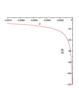
Figure 1: Singularity of the first derivative of the thermodynamic potential $u$ with respect to the chemical potential.

Accordingly, we can conclude that there exists a first-order phase transition as the chemical potential approaches zero.

We now investigate the geometric properties of the equilibrium manifold. It is convenient to rewrite the thermodynamic potential (43) in terms of the critical temperature. To this end, in the definition of $u$ we consider the maximum particle number, $u=U/N_{max}$, to obtain

$$u=\frac{3}{2\zeta}k_{{}_{B}}\frac{T^{5/2}}{T_{c}^{3/2}}g_{\frac{5}{2}}(z)\ ,$$ (44)

which for convenience we rewrite as

$$u=\frac{3}{2\zeta}\,k_{{}_{B}}\,T_{c}\,t^{5/2}\,g_{\frac{5}{2}}(z)\ ,\quad z=e^{\frac{\mu}{k_{{}_{{}_{B}}}T_{c}t}}\ ,\quad t=\frac{T}{T_{c}}\ .$$ (45)

This is the fundamental equation that describes the transition of a Bose gas into a Bose-Einstein condensate in the limit $t\rightarrow 1$ and $\mu\rightarrow 0$. According to the results of GTD, for the calculation of the metric (16) of the equilibrium manifold, we identify $u$ with the thermodynamic potential $\Phi$ and $E^{a}=(t,\mu)$. Then, a straightforward computation leads to the following metric components

$$g_{tt}=\frac{9}{32\zeta^{2}}\left(5T_{c}tg_{\frac{5}{2}}-2\mu g_{\frac{3}{2}}\right)\left(15T_{c}^{2}t^{2}g_{\frac{5}{2}}-12T_{c}t\mu g_{\frac{3}{2}}+4\mu^{2}g_{\frac{1}{2}}\right)\ ,$$ (46)

$$g_{t\mu}=\frac{45}{32\zeta^{2}}t^{2}g_{\frac{5}{2}}\left(3T_{c}tg_{\frac{3}{2}}-2\mu g_{\frac{1}{2}}\right)\ ,$$ (47)

$$g_{\mu\mu}=\frac{9}{4\zeta^{2}T_{c}}g_{\frac{3}{2}}g_{\frac{1}{2}}\ ,$$ (48)

where for the sake of simplicity we set $k_{{}_{B}}=1$ and drop the argument of the Bose integral $g_{n}\left(e^{\frac{\mu}{T_{c}t}}\right)$. It is easy to check that the determinant of this metric is non-vanishing, indicating that the geometry is well defined. The corresponding curvature tensor can then be computed, but its final expression cannot be written in a compact form. Nevertheless, we performed a detailed numerical analysis of the behavior of the curvature scalar and found that there is a singularity in the limit $t=1$ and $\mu\rightarrow 0$. Figure 2 illustrates this behavior.

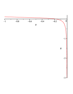
Figure 2: Singularity of the curvature scalar near the origin $\mu=0$ for $t=1$. Here we use the value $T_{c}=1$ for simplicity.

This result shows that the values at which the Bose-Einstein condensation takes place, correspond to a curvature singularity of the corresponding equilibrium manifold.

V Conclusions

In the present work, we analyzed the properties of the space of equilibrium states of the ideal quantum gases in the context of geometrothermodynamics. First, we derived the fundamental equations from which we can obtain all the thermodynamic properties of the gases. It was established that a Boltzmann gas, whose components are identical classical particles, possesses a flat equilibrium manifold, indicating the lack of thermodynamic interaction. This is in accordance with our intuitive interpretation of thermodynamic interaction which is associated with the presence of a potential term in the corresponding Hamiltonian.

On the other hand, our analysis shows that Fermi and Bose quantum gases possess a non-flat equilibrium space, although the corresponding Hamiltonian does not contain a potential term. This result shows that the curvature of the equilibrium space is able to detect the “effective” thermodynamic interaction which arises from the quantum nature of the gas components. We interpret this result as an indication in favor of considering the curvature of the equilibrium manifold as a measure of the thermodynamic interaction, instead of the intuitive notion based upon the presence of a potential term in the Hamiltonian.

We also analyzed the Bose-Einstein condensation from the point of view of GTD. First, we established a particular fundamental equation that allows us to apply the Ehrenfest definition to interpret the Bose-Einstein condensation as a first-order phase transition of an ideal Bose gas. The same fundamental equation is then used to derive the geometric properties of the corresponding equilibrium manifold. We found that the curvature is non-zero, indicating the presence of thermodynamic interaction, and that there exists a curvature singularity at exactly that point in the equilibrium manifold where the Bose-Einstein condensation takes place. This result indicates that GTD is able to correctly describe the thermodynamic properties of ideal classical and quantum gases.

Ideal quantum gases have been investigated from the point of view information geometric theory amari85 ; janmru90 ; ooh99 ; mirmoh11 . Using the second moments of the energy and particle number fluctuations as the components of a thermodynamic metric, in janmru90 , it was shown that the corresponding curvature can be used as a measure of stability. For bosons, for example, the curvature tends to zero at the classical limit and diverges in the condensation region. The results we obtained in GTD are consistent with this information geometric approach. A quantum ideal gas obeying Gentile’s intermediate statistics was investigated in ooh99 . The thermodynamic curvature is constructed such that it depends on the fugacity and the number of particles in a state, and it turns out to contain information about the stability properties of the system. In the classical limit of a Boltzmann gas, however, the curvature does not vanish as expected, but contains contributions from the quantum statistical character of the gas. A different intermediate statistics for deformed bosons and deformed fermions was investigated in mirmoh11 . The corresponding singular points of the curvature were shown to be related with condensation even in the case of deformed bosons.

Finally, for the sake of comparison, we used thermodynamic geometry in which the metric is given as the Hessian for different thermodynamic potentials. In the case of the entropy, the curvature is non-zero with a singularity at a value of $\mu$ that does not coincide with the Bose-Einstein condensate limiting value. If, instead, the internal energy is used as thermodynamic potential the corresponding metric is flat, indicating that no interaction is present. Both results are inconsistent with the thermodynamic properties of ideal quantum gases.

References

- (1) T. Frankel, The Geometry of Physics: An Introduction (Cambridge University Press, Cambridge, UK, 1997).
- (2) C. N. Yang and R. L. Mills, Phys. Rev. 96, 191 (1954).
- (3) C. R. Rao, Bull. Calcutta Math. Soc. 37, 81 (1945).
- (4) S. Amari, Differential-Geometrical Methods in Statistics (Springer-Verlag, Berlin, 1985).
- (5) F. Weinhold, J. Chem. Phys. 63, 2479, 2484, 2488, 2496 (1975); 65, 558 (1976).
- (6) G. Ruppeiner, Phys. Rev. A 20, 1608 (1979).
- (7) G. Ruppeiner, Rev. Mod. Phys. 67, 605 (1995); 68, 313 (1996).
- (8) H. Quevedo, J. Math. Phys. 48, 013506 (2007).
- (9) H. B. Callen, Thermodynamics and an Introduction to Thermostatics (John Wiley & Sons, Inc., New York, 1985).
- (10) V. I. Arnold, Mathematical methods of classical mechanics (Springer Verlag, New York, 1980).
- (11) R. Hermann, Geometry, physics and systems (Marcel Dekker, New York, 1973).
- (12) K. Huang, Statistical Mechanics (John Wiley & Sons, Inc., New York, 1987).
- (13) H. Quevedo, A, Sánchez and A. Vázquez, Relativistic like structure of classical thermodynamics, Gen. Rel. Grav. (2015); in press.
- (14) W. Greiner, L. Neise and H. Stöcker, Thermodynamics and Statistical Mechanics (Springer Verlag, New York, 1995).
- (15) L. Olivares-Quiroz and V. Romero-Rochin, J. Phys. B: At. Mol. Opt. Phys. 43, 205302 (2010).
- (16) A. Vázquez, H. Quevedo, and A. Sánchez, J. Geom. Phys. 60, 1942 (2010).
- (17) H. Janyszek and R. Mrugala, J. Phys. A: Math. Gen. 23, 467 (1990).
- (18) H. Oshima, T. Obata and H. Hara, J. Phys. A: Math. Gen. 32, 6373 (1999).
- (19) B. Mirza and H. Mohammadzadeh, J. Phys. A: Math. Gen. 44, 475003 (2011).