aDepartment of Mathematics, Middle East Technical University, 06800, Ankara, Turkey
bDepartment of Mathematics, Gazi University, 06500, Teknikokullar, Ankara, Turkey
Abstract
In the present study, we investigate the existence of Li-Yorke chaos in the dynamics of shunting inhibitory cellular neural networks (SICNNs) on time scales. It is rigorously proved by taking advantage of external inputs that the outputs of SICNNs exhibit Li-Yorke chaos. The theoretical results are supported by simulations, and the controllability of chaos on the time scale is demonstrated by means of the Pyragas control technique. This is the first time in the literature that the existence as well as the control of chaos are provided for neural networks on time scales.
Keywords: Shunting inhibitory cellular neural networks; Time scales; Li-Yorke chaos; Proximality; Frequent separation; Chaos control
1 Introduction
Cellular neural networks (CNNs) have been paid much attention starting with the studies of Chua and Yang [1, 2]. Exceptional role in psychophysics, speech, perception, robotics, adaptive pattern recognition, vision, and image processing has been played by shunting inhibitory cellular neural networks (SICNNs), which was introduced by Bouzerdoum and Pinter [3]. The reader is referred to [4]-[8] for the applications of SICNNs. Another subject that is also popular is the theory of time scales, which is first presented by Hilger [9]. This theory has many applications in various scientific fields, and neural networks are no exception [10]-[26].
The first mathematically rigorous definition of chaos was introduced by Li and Yorke [27]. It was shown in [27] that if a map on an interval has a point of period three, then it possesses chaos in the sense of Li-Yorke. The presence of an uncountable scrambled set is a distinguishing feature of the Li-Yorke chaos. It was indicated in [28] that if a map on a compact interval has a two point scrambled set, then it possesses an uncountable scrambled set. Li-Yorke sensitivity, which links the Li-Yorke chaos with the notion of sensitivity, was studied by Akin and Kolyada [29]. It was proved in [30] that the presence of positive topological entropy implies chaos in the sense of Li-Yorke. According to Marotto [31], a multidimensional continuously differentiable map is Li-Yorke chaotic provided that it has a snap-back repeller. On the other hand, Marotto’s Theorem was utilized by Li et al. [32] to demonstrate the existence of Li-Yorke chaos in a spatiotemporal chaotic system. Moreover, Li-Yorke chaos on several spaces in connection with the cardinality of its scrambled sets was studied within the scope of the paper [33], and generalizations of Li-Yorke chaos to mappings in Banach spaces and complete metric spaces were provided in [34]-[36]. The presence of Li-Yorke chaos in dynamic equations on time scales was first studied in the paper [37]. The extension mechanism of chaos in continuous-time systems can be found in the studies [38]-[46].
To the best of our knowledge, the existence of chaos has never been achieved for neural networks on time scales in the literature before. The main novelty of the present paper is the consideration of chaos for neural networks on time scales. We develop the concept of Li-Yorke chaos for SICNNs on time scales and prove its existence rigorously by making use of the reduction technique to impulsive differential equations, which was introduced by Akhmet and Turan [47]. The results are appropriate to obtain chaotic SICNNs on time scales with arbitrary high number of cells. Another novelty of the present study is the control of chaos on time scales. The Pyragas control method [48]-[51] is utilized to control the chaos in the dynamics of SICNNs on time scales. Our results show that the Pyragas control method is suitable to control chaos not only in continuous-time or discrete-time systems, but also in systems on time scales.
It was revealed in the papers [52, 53] that chaotic dynamics is inevitable for brain activities, and it was suggested by Guevara et al. [54] that chaotic behavior may be responsible for dynamical diseases such as schizophrenia, insomnia, epilepsy and dyskinesia. Besides, the presence of chaos in neural networks is useful for separating image segments [55], information processing [56, 57] and synchronization [58]-[61], and it can improve the performance of CNNs on problems that have local minima in energy (cost) functions, since chaotic behavior of CNNs can help the network avoid local minima and reach the global optimum [62]. Moreover, chaos is an important tool in CNNs for the studies of chaotic communication [63]-[66] and combinatorial optimization problems [67].
Let us describe the model of SICNNs in its most original form [3]. Consider a two dimensional grid of processing cells arranged into rows and columns, and let denote the cell at the position of the lattice. In SICNNs, neighboring cells exert mutual inhibitory interactions of the shunting type. The dynamics of a cell are described by the following nonlinear ordinary differential equation,
(1.2)
where is the activity of the cell is the external input to the cell the constant represents the passive decay rate of the cell activity; is the coupling strength of postsynaptic activity of the cell transmitted to the cell the activation function is a positive continuous function representing the output or firing rate of the cell and the neighborhood of the cell is defined as
Motivated by the deficiency of mathematical methods for the investigation of chaos in neural networks on time scales, in the present study, we will consider the following SICNN,
(1.3)
where and the sequence is strictly increasing such that as The external input is defined through the equation for such that the sequence is generated by the map
(1.4)
where is a continuous function and is a compact subset of We assume that and In this paper, the chaotic dynamics of SICNN (1.3) is investigated. We rigorously prove the existence of Li-Yorke chaos in the network (1.3) provided that the map (1.4) is Li-Yorke chaotic. One of the significant features of the obtained chaos is its controllability. We also demonstrate the control of the obtained chaos by means of the Pyragas control technique [48].
The dynamics of (1.3) is essentially non-autonomous, and it is difficult to verify the ingredients of chaos for unspecified time scales. That is the reason why we utilize the time scale introduced by Akhmet and Turan [47, 68] as well as the reduction technique to impulsive differential equations [47].
Artificial neural networks on time scales of the form can be useful to model neural processes whose instantaneous rate of change cannot be expressed through a differential equation, i.e., not achievable for differential equation analysis. In other words, one can take into account the intervals as the ones in which the neural processes are achievable so that the instantaneous rate (differential equation) can be obtained experimentally, and the intervals can be considered as the ones in which the neural process cannot be achieved. On the other hand, neural processes on time scales which are unions of disjoint compact intervals can be interpreted as activities that work intermittently, i.e., activities that proceed at certain disjoint time intervals and discontinue in between. This type of behavior can be observed in many biological neural activities. For instance, there exist hearth interneurons and motor neurons in the leech whose activities last for about 6 seconds and then the neurons become silent for about 6 seconds [69]. Besides, in Xenopus tadpoles, fictive swimming activity can be initiated by brief touch and swimming normally stops when the tadpole contacts an object or the water surface with its head [70]-[72]. The role of inhibitory reticulospinal neurons for this behavior was investigated by Perrins et al. [72]. In addition to these, intermittent external inputs are effective tools for the treatment of neurological disorders. It was demonstrated by Boggs et al. [73] that intermittent electrical stimulation of the pudendal nerve can restore bladder emptying. Moreover, the potential of intermittent vagus nerve stimulation to treat chronic hypertension and cardiac arrhythmias was studied by Annoni et al. [74].
The existence and stability of periodic, almost periodic and anti-periodic solutions of neural networks on time scales have been extensively investigated in the literature [15]-[26]. In particular, the papers [21]-[23] were concerned with the dynamics of SICNNs on time scales. The existence and global exponential stability of anti-periodic solutions of impulsive SICNNs with distributed delays on time scales were studied by Li and Shu [21] by means of the coincidence degree method and Lyapunov functionals. On the other hand, periodic solutions of SICNNs of neutral type with time-varying delays in the leakage term on time scales were considered in the paper [22]. Moreover, the existence and asymptotic stability of almost periodic solutions for SICNNs with time-varying and continuously distributed delays on time scales are studied in [23] without assuming the global Lipschitz conditions of activation functions. The concept of almost periodicity was also considered within the scope of the paper [47] by using the reduction technique to impulsive differential equations, and the results of [47] can be developed for neural networks on time scales. However, chaos in neural networks on time scales was not taken into account in these studies. In the papers [75, 76], SICNNs with impulsive effects were investigated, and it was numerically demonstrated that chaos exists in such networks without a theoretical support. The presence of chaos in continuous-time models of SICNNs with impulses, delay and chaotic/almost periodic postsynaptic currents was rigorously proved and supported by simulations in [43]-[46]. Contrarily, in the present paper, we rigorously prove the existence of chaos in SICNNs on time scales. The control of the chaos on time scales is another novelty of our study.
The rest of the paper is organized as follows. In Section 2, some basic concepts about differential equations on time scales are provided, and sufficient conditions for the existence of chaos are given. We investigate the existence, uniqueness and attractiveness feature of the bounded solutions of the network (1.3) in Section 3. The main result of the present study is indicated in Section 4, where we rigorously prove the presence of Li-Yorke chaos in the dynamics of (1.3). An illustrative example is presented in Section 5, and a chaos control technique is numerically demonstrated in Section 6 by means of the Pyragas control method. Finally, Section 7 is devoted for conclusions.
2 Preliminaries
The basic concepts about differential equations on time scales are as follows [10, 11]. A time scale is a nonempty closed subset of On a time scale , the forward and backward jump operators are defined as and respectively. A point is called right-scattered if and right-dense if . Similarly, if then is called left-scattered, and otherwise it is called left-dense. We say that a function is rd-continuous provided it is continuous at each right-dense point and its left-sided limits exist at each left-dense point At a right-scattered point the -derivative of a continuous function is defined as On the other hand, at a right-dense point we have provided that the limit exists.
We suppose that the time scale used in SICNN (1.3) satisfies the property, i.e., there exists a positive number such that whenever Under this assumption, there exists a natural number such that for all where [47]. It is worth noting that the points , are left-scattered and right-dense, and the points , are right-scattered and left-dense on the time scale Moreover, , , and for any except at the points
Let us assume without loss of generality that and define the substitution [47] on the set as
(2.7)
One can confirm that the function is one-to-one and onto, and It was shown by Akhmet and Turan [47] that and provided that where
(2.10)
and the sequence is defined through the equation for each The function is piecewise continuous with discontinuities of the first kind at the points such that where The sequence is periodic, i.e., for all and Moreover, if a function is periodic on then is periodic, and vice versa.
One of the significant results mentioned in the paper [47] concerning the functions defined on and is as follows. Denote by the set of all rd-continuous functions and let be the set of all continuously differentiable functions on assuming that the functions have a one sided derivative at Moreover, a function is an element of the set if it is left-continuous on and continuous on and it has discontinuities of the first kind at the points The function belongs to the set if both and are elements of where It was proved in [47] that a function belongs to if and only if belongs to
Applying the transformation to (2.13) we obtain the following impulsive network,
(2.16)
where and
In the remaining parts of the paper, we will make use of the norm where
The following conditions are required throughout the paper.
(C1)
for all and
(C2)
where
(C3)
There exists a positive number such that
(C4)
There exists a positive number such that for all
Let us define in the case that and are numbers such that for some integers and with On the other hand, if for some integer then take One can verify under the conditions and that for each there exist positive numbers such that
Suppose that where and In the remaining parts of the paper, we will denote and and
The following conditions are also needed.
(C5)
(C6)
In the next section, we will deal with the existence, uniqueness and attractiveness property of the bounded solutions of SICNN (1.3).
3 Bounded solutions
According to the results of [77, 78], a bounded on function is a solution of the impulsive system (2.16) if and only if the equation
is valid.
The existence of bounded on solutions of (2.16) is considered in the next assertion.
Lemma 3.1
Suppose that the conditions are fulfilled. For each solution of (1.4), there exists a unique bounded on solution of (2.16) such that
Proof. Fix a solution of (1.4) and take into account the set consisting of functions of the form which have discontinuities at the points such that where The set is complete [77].
Define an operator on as
where
If then one can confirm that
The last inequality implies that
Therefore,
On the other hand, for any we have
(3.21)
One can show by using (3.21) that Thus, according to condition the operator is a contraction.
Consequently, there exists a unique bounded on solution of (2.16) such that
It is worth noting that for a given solution of (1.4), Lemma 3.1 implies that the function satisfying and is the unique solution of (1.3), which is bounded on such that
A bounded solution of (1.3) is said to attract another solution of the same network if as The next lemma is devoted to the attractiveness feature of the bounded solutions of (1.3).
Lemma 3.2
If the conditions are valid, then for a fixed solution of (1.4), the bounded solution of (1.3) attracts all other solutions of the network.
Proof. Consider an arbitrary solution of (1.3) such that where and Assume without loss of generality that for any and let and In this case, for the solutions and of (2.16) satisfy the relation
It can be verified by using the last equation that
where
Benefiting from the Gronwall-Bellman Lemma for piecewise continuous functions [77], we obtain for that
Condition implies that as Hence, as
The presence of Li-Yorke chaos in SICNN (1.3) will be investigated in the next section.
4 Li-Yorke chaos
The map (1.4) is called Li-Yorke chaotic on if [27, 29]:
(i) For every natural number there exists a periodic point of in
(ii) There is an uncountable set the scrambled set, containing no periodic points, such that for every with we have and
(iii) For every and a periodic point we have
Denote by the set of all sequences obtained by equation (1.4). We say that a pair of sequences is proximal if and it is frequently separated if
Let be the collection of all bounded solutions of (1.3) such that A pair is proximal if for an arbitrary small positive number and an arbitrary large natural number there exists an integer such that for all
On the other hand, the pair is frequently -separated if there exist numbers and infinitely many disjoint intervals each with a length no less than such that for each from these intervals. Moreover, , is a Li-Yorke pair if it is proximal and frequently -separated for some positive numbers and
The SICNN (1.3) is called Li-Yorke chaotic if:
(i) There exists a periodic solution of (1.3) for each
(ii) There exists an uncountable set the scrambled set, which does not contain any periodic solution, such that any pair of different solutions of (1.3) inside is a Li-Yorke pair;
(iii) For any and any periodic solution the pair , is frequently -separated for some positive numbers and
One can confirm that the sequence is periodic, where Suppose that and We will denote by the number of the terms of the sequence that belong to the interval It can be verified that for any real numbers such that
The proximality feature of bounded solutions of SICNN (1.3) will be mentioned in the following lemma.
Lemma 4.1
Assume that the conditions are satisfied. If a pair of sequences is proximal, then the same is true for the pair
Proof.
Throughout the proof, let us denote
and
Assume that is a real number which satisfies the inequality
Fix an arbitrary small number and an arbitrary large natural number such that
Since the pair is proximal, there exists an integer such that
for
The bounded solutions of (2.16) satisfy the relation
Therefore, for we have that
(4.26)
Define the function The inequality (4.26) implies that
Making use of the Gronwall’s Lemma for piecewise continuous functions, one can obtain that
Since the inequality
is valid for any real numbers and with we have
Hence, it can be verified that
For utilizing the inequality
we attain that
Thus, for
Consequently, the pair is proximal.
The next lemma is devoted to the frequent separation feature in SICNN (1.3).
Lemma 4.2
Under the conditions if a pair of sequences is frequently separated, then the pair of bounded solutions is frequently -separated for some positive numbers and
Proof. Since the pair is frequently separated, there exists a positive number and a sequence of integers satisfying as such that
Fix a natural number If then the bounded solutions and of (2.16) satisfy the relation
Thus, it can be verified that
The last inequality yields
where
Now, let be the minimum of the numbers and
First of all, suppose that
for some and denote
If belongs to the interval then we have that
Hence, one can obtain that
On the other hand, if
then it can be shown in a similar way that the inequality is valid also for
Therefore, for Clearly, the intervals are disjoint. Consequently, the pair of bounded solutions is frequently -separated.
The main result of the present paper is as follows.
Theorem 4.1
If the conditions are valid and the map (1.4) is Li-Yorke chaotic on then SICNN (1.3) is Li-Yorke chaotic.
Proof.
Let be a periodic solution of the map (1.4) for some natural number In this case, the external input is periodic, where It can be shown that the bounded solution of (1.3) is periodic. Therefore, there exists a periodic solution of (1.3) for each natural number
Denote by the set consisting of bounded solutions of (1.3) for which where is the scrambled set of (1.4). One can confirm that the set is uncountable and no periodic solutions take place inside
Using the Lemmas 4.1 and 4.2, one can confirm that any pair of different solutions inside is a Li-Yorke pair, i.e. is a scrambled set. Lemma 4.2 implies also that for any solution and any periodic solution the pair is frequently -separated for some positive numbers and Consequently, the network (1.3) is Li-Yorke chaotic.
In the following section, we will present an example, which supports the result of Theorem 4.1.
5 An example
Consider the following SICNN,
(5.27)
where for for and
Notice that the time scale satisfies the property with In (5.27), for each and we will use the following coupling strengths,
whenever the cells belong to More precisely, for fixed and the coupling strengths are taken to be equal to each other in cases where belongs to For instance, Furthermore, for each and we take for where the sequence is generated by the logistic map
(5.28)
The map (5.28) is chaotic in the sense of Li-Yorke for the values of the parameter between and [27]. Moreover, for these values of the parameter, the interval is invariant under the iterations of the map [79].
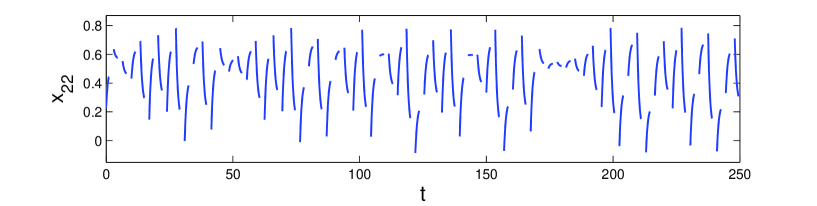
Let us take in (5.28). One can verify that the conditions are valid for (5.27) with Thus, according to Theorem 4.1, SICNN (5.27) is Li-Yorke chaotic. We take and represent in Figure 1 the -coordinate of (5.27) corresponding to the initial data Figure 1 supports the result of Theorem 4.1 such that the network (5.27) possesses Li-Yorke chaos.
Figure 1: Time series of the coordinate of SICNN (5.27). The figure manifests that the network behaves chaotically.
In the next section, we will demonstrate how to control the chaos of SICNN (5.27) numerically by using the Pyragas control technique [48].
6 Control of chaos
In the literature, control of chaos is understood as the stabilization of unstable periodic orbits embedded in a chaotic attractor. The studies on the control of chaos originated with Ott, Grebogi and Yorke [80]. The Ott-Grebogi-Yorke (OGY) control method depends on the usage of small time-dependent perturbations in an accessible system parameter to stabilize an already existing periodic orbit, which is initially unstable. Another well known technique for the control of chaotic systems is the Pyragas method [48], which is known as delayed feedback control.
The source of the chaotic outputs generated by SICNN (5.27) is the logistic map (5.28). In this section, we will show that the chaos of (5.27) can be controlled by applying the Pyragas control technique to the map (5.28). More precisely, we will stabilize the unstable periodic solution of (5.27) by performing the Pyragas method to (5.28) around the fixed point of the map.
The chaos control techniques such as the Pyragas and OGY methods are suitable for either continuous-time or discrete-time systems [48, 50, 80, 81]. However, to the best of our knowledge, there is no chaos control technique for dynamics on time scales. This is the main reason why we apply the Pyragas control to the logistic map in order to control the chaos of (5.27). It is worth noting that the OGY algorithm can also be applied to the logistic map to control the chaos of (5.27).
Now, let us describe the Pyragas control technique for the logistic map (5.28). The aim in this method is to stabilize the unstable fixed point of (5.28) by using the delayed feedback control algorithm
(6.29)
where is the feedback gain [48, 49, 51]. According to the results of the paper [49], the nonzero fixed point becomes stable for
and the optimal value of the feedback gain, which leads to the fastest convergence of nearby initial conditions is
It was mentioned in [49] that the algorithm (6.29) is successful if the initial data are sufficiently close to the fixed point, and solutions of (6.29) can escape to infinity for some initial data from the chaotic attractor of (5.28). In order to guarantee the stabilization for any initial data, Pyragas and Pyragas [49] proposed that the condition
(6.30)
has to be satisfied for a suitably chosen small positive number which can be determined only numerically. The inequality (6.30) is used to estimate the strength of the perturbation if it would be applied at a given iteration step On the other hand, the condition
(6.31)
is required to avoid the stabilization of the zero fixed point [49].
In the Pyragas control method, at each iteration step after the control mechanism is switched on, we consider the map (6.29) with a chosen value of between and provided that (6.30) and (6.31) are valid. Otherwise, we take and wait until both (6.30) and (6.31) are satisfied. If this is the case, the control of chaos is not achieved
immediately after switching on the control mechanism. Instead, there is a transition time that depends on the ergodic properties of (5.28) before the fixed point is stabilized.
Now, we will apply the Pyragas control technique to the logistic map (5.28) with around the fixed point to control the chaos of (5.27). For that purpose, we take into account the following auxiliary network,
(6.32)
where and is a solution of (6.29). The network (6.32) is the control network conjugate to (5.27). The time scale activation function passive decay rates and coupling strengths in (6.32) are the same with the ones used in (5.27). For each and the external inputs in (6.32) are defined as for
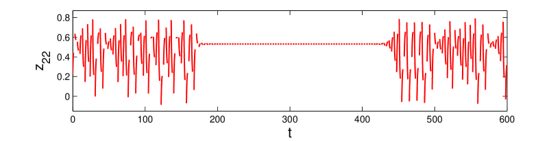
Figure 2 shows the -coordinate of (6.32) corresponding to the initial data and The control mechanism is switched on at and switched off at In the simulation, we take and make use of the optimum value of the feedback gain It is seen in Figure 2 that the unstable periodic solution of (5.27) is stabilized. The control becomes dominant approximately at and its effect prolongs approximately till after which chaos emerges again and irregular behavior reappears. It is worth noting that the stabilization does not occur immediately after switching on the control mechanism, but rather there is a transition time. The simulation result demonstrates that it is sufficient to stabilize an unstable periodic orbit of the logistic map (5.28) to control the chaos of SICNN (5.27).
Figure 2: Stabilization of the unstable periodic solution of SICNN (5.27) by means of the conjugate control network (6.32). The chaos of (5.27) is controlled by applying the Pyragas control technique to the logistic map (5.28) around the fixed point The values and are utilized in the simulation. The control mechanism is switched on at and switched off at
7 Conclusions
The present study is concerned with the existence of Li-Yorke chaos in SICNNs on time scales. We rigorously prove the ingredients of Li-Yorke chaos, proximality and frequent separation, by taking advantage of the external inputs. This is the first time in the literature that chaos is obtained for neural networks on time scales. Our results reveal that external inputs are capable of generating chaotic outputs on time scales. The presented technique can be used to obtain chaotic SICNNs on time scales without any restriction in the number of cells.
Another significant result of our paper is the control of the chaos on time scales. The presence of unstable periodic motions embedded in the chaotic attractor is evidenced by means of the Pyragas control technique [48, 49]. It is numerically demonstrated that the Pyragas method is appropriate for controlling chaos not only in discrete and continuous-time systems, but also in systems on time scales.
The detection of chaotic behavior in neural networks is of great interest since it may provide the opportunity to understand how the brain and the rest of the nervous system works. We believe that the presented technique will shed light on the mathematical investigation of neural processes that work intermittently [69, 72, 82]. Moreover, our results can provide further research areas in neural activities that are achievable at certain time intervals. The problem of period-doubling route to chaos [83, 84] by neural networks on time scales can be considered in the future through the presented method. Our approach can also be useful for designing secure communication systems [63, 85, 86, 87], and it can be improved for other kinds of recurrent networks such as Hopfield and Cohen-Grossberg neural networks [88, 89].
Acknowledgments
This work is supported by the 2219 scholarship programme of TÜBİTAK, the Scientific and Technological Research Council of Turkey.
[3] A. Bouzerdoum, R.B. Pinter, Shunting inhibitory cellular neural networks: derivation and stability analysis. IEEE Trans. Circuits Systems I Fund. Theory. and Appl. 40 (1993) 215–221.
[4] A. Bouzerdoum, B. Nabet, R.B. Pinter, Analysis and analog implementation of directionally sensitive shunting inhibitory cellular neural networks, in: Visual Information Processing: From Neurons to Chips, Proc. SPIE 1473, 1991, pp. 29–38.
[5] A. Bouzerdoum, R.B. Pinter, Nonlinear lateral inhibition applied to motion detection in the fly visual system, in: R.B. Pinter, B. Nabet (Eds.), Nonlinear Vision, CRC Press, Boca Raton, FL, 1992, pp. 423–450.
[6] A. Bouzerdoum, R.B. Pinter, A shunting inhibitory motion detector that can account for the functional characteristics of fly motion sensitive interneurons, Proceedings of IJCNN International Joint Conference on Neural Networks, 1990, pp. 149–153.
[7] R.B. Pinter, R.M. Olberg, E. Warrant, Luminance adaptation of preferred object size in identified dragonfly movement detectors, Proceedings of IEEE International Conference on Systems, Man and Cybernetics, 1989, pp. 682–686.
[8] H.N. Cheung, A. Bouzerdoum, W. Newland, Properties of shunting inhibitory cellular neural networks for colour image enhancement, Proceedings of 6th International Conference on Neural Information Processing, Perth, Western Australia, 1999, pp. 1219–1223.
[9] S. Hilger, Ein Maßkettenkalkül mit Anwendung auf Zentrumsmanningfaltigkeiten, PhD thesis, Universität Würzburg, 1988.
[10] M. Bohner, A. Peterson, Dynamic Equations on Time Scales: An Introduction with Applications, Birkhäuser, Boston, 2001.
[11] V. Lakshmikantham, S. Sivasundaram, B. Kaymakcalan, Dynamic Systems on Measure Chains, Kluwer Academic Publishers, Netherlands, 1996.
[12] J. Zhang, M. Fan, H. Zhu, Periodic solution of single population models on time scales, Mathematical and Computer Modelling 52 (2010) 515–521.
[13] C.C. Tisdell, A. Zaidi, Basic qualitative and quantitative results for solutions to nonlinear, dynamic equations on time scales with an application to economic modelling, Nonlinear Analysis 68 (2008) 3504–3524.
[14] Y. Su, Z. Feng, Homoclinic orbits and periodic solutions for a class of Hamiltonian systems on time scales, Journal of Mathematical Analysis and Applications 411 (2014) 37–62.
[15] B. Zhou, Q. Song, H. Wang, Global exponential stability of neural networks with discrete and distributed delays and general activation functions on time scales, Neurocomputing 74 (2011) 3142–3150.
[16] C. Wang, Almost periodic solutions of impulsive BAM neural networks with variable delays on time scales, Commun. Nonlinear. Sci. Numer. Simulat. 19 (2014) 2828–2842.
[17] H. Zhou, Z. Zhou, W. Jiang, Almost periodic solutions for neutral type BAM neural networks with distributed leakage delays on time scales, Neurocomputing 157 (2015) 223–230.
[18] C. Xu, Q. Zhang, Existence and global exponential stability of anti-periodic solutions of high-order bidirectional associative memory (BAM) networks with time-varying delays on time scales, Journal of Computational Science 8 (2015) 48–61.
[19] X. Chen, Q. Song, Global stability of complex-valued neural networks with both leakage time delay and discrete time delay on time scales, Neurocomputing 121 (2013) 254–264.
[20] Y. Li, L. Yang, W. Wu, Anti-periodic solutions for a class of Cohen-Grossberg neural networks with time-varying delays on time scales, International Journal of Systems Science 42 (2011) 1127–1132.
[21] Y. Li, J. Shu, Anti-periodic solutions to impulsive shunting inhibitory cellular neural networks with distributed delays on time scales, Commun. Nonlinear Sci. Numer. Simulat. 16 (2011) 3326–3336.
[22] Y. Li, L. Wang, Y. Fei, Periodic solutions for shunting inhibitory cellular neural networks of neutral type with time-varying delays in the leakage term on time scales, Journal of Applied Mathematics 2014 (2014) 496396.
[23] Y. Li, C. Wang, Almost periodic solutions of shunting inhibitory cellular neural networks on time scales, Commun. Nonlinear Sci. Numer. Simulat. 17 (2012) 3258–3266.
[24] L. Yang, Y. Li, Existence and exponential stability of periodic solution for stochastic Hopfield neural networks on time scales, Neurocomputing 167 (2015) 543–550.
[25] Y. Liu, Y. Yang, T. Liang, L. Li, Existence and global exponential stability of anti-periodic solutions for competitive neural networks with delays in the leakage terms on time scales, Neurocomputing 133 (2014) 471–482.
[26] Q. Cheng, J. Cao, Synchronization of complex dynamical networks with discrete time delays on time scales, Neurocomputing 151 (2015) 729–736.
[27] T.Y. Li, J.A. Yorke, Period three implies chaos, Amer. Math. Monthly 87 (1975) 985–992.
[28] M. Kuchta, J. Smítal, Two point scrambled set implies chaos, European Conference on Iteration Theory (ECIT 87), World Sci. Publishing, Singapore, 1989, pp. 427–430.
[29] E. Akin, S. Kolyada, Li-Yorke sensitivity, Nonlinearity 16 (2003) 1421–1433.
[30] F. Blanchard, E. Glasner, S. Kolyada, A. Maass, On Li-Yorke pairs, J. Reine Angew. Math. 2002 (2002) 51–68.
[32] P. Li, Z. Li, W.A. Halang, G. Chen, Li-Yorke chaos in a spatiotemporal chaotic system, Chaos, Solitons and Fractals 33 (2007) 335–341.
[33] J.L.G. Guirao, M. Lampart, Li and Yorke chaos with respect to the cardinality of the scrambled sets, Chaos, Solitons and Fractals 24 (2005) 1203–1206.
[34] P. Kloeden, Z. Li, Li-Yorke chaos in higher dimensions: a review, Journal of Difference Equations and Applications 12 (2006) 247–269.
[35] Y. Shi, G. Chen, Chaos of discrete dynamical systems in complete metric spaces, Chaos, Solitons & Fractals 22 (2004) 555–571.
[36] Y. Shi, G. Chen, Discrete chaos in Banach spaces, Science in China, Ser. A: Mathematics 48 (2005) 222–238.
[37] M. Akhmet, M.O. Fen, Li-Yorke chaos in hybrid systems on a time scale, Int. J. Bifurcation and Chaos (in press).
[38] M.U. Akhmet, Devaney’s chaos of a relay system, Commun. Nonlinear Sci. Numer. Simulat. 14 (2009) 1486–1493.
[39] M.U. Akhmet, Li-Yorke chaos in the system with impacts, J. Math. Anal. Appl. 351 (2009) 804–810.
[40] M.U. Akhmet, Creating a chaos in a system with relay, Int. J. Qual. Theory. Differ. Equat. Appl. 3 (2009) 3–7.
[44] M.U. Akhmet, M.O. Fen, Attraction of Li-Yorke chaos by retarded SICNNs, Neurocomputing 147 (2015) 330–342.
[45] M. Akhmet, M.O. Fen, Replication of Chaos in Neural Networks, Economics and Physics, Springer-Verlag, Berlin, Heidelberg, 2016.
[46] M. Akhmet, M.O. Fen, A. Kıvılcım, Li-Yorke chaos generation by SICNNs with chaotic/almost periodic postsynaptic currents, Neurocomputing 173 (2016) 580–594.
[47] M.U. Akhmet, M. Turan, The differential equations on time scales through impulsive differential equations, Nonlinear Analysis 65 (2006) 2043–2060.
[48] K. Pyragas, Continuous control of chaos by self-controlling feedback, Phys. Lett. A 170 (1992) 421–428.
[49] V. Pyragas, K. Pyragas, Modification of delayed feedback control using ergodicity of chaotic systems, Lithuanian Journal of Physics 50 (2010) 305-316.
[50] J.M. Gonzalés-Miranda, Synchronization and Control of Chaos, Imperial College Press, London, 2004.
[51] I. Zelinka, S. Celikovsky, H. Richter, G. Chen (Eds.), Evolutionary Algorithms and Chaotic Systems, Springer-Verlag, Berlin, Heidelberg, 2010.
[52] W.J. Freeman, Tutorial on neurobiology: from single neurons to brain chaos, Int. J. Bifur. Chaos 2 (1992) 451–482.
[53] C.A. Skarda, W.J. Freeman, Chaos and the new science of the brain, Concepts Neurosci. 1 (1990) 275–285.
[54] M.R. Guevara, L. Glass, M.C. Mackey, A. Shrier, Chaos in neurobiology, IEEE Trans. Syst. Man Cybern. SMC-13 (1983) 790–798.
[55] M. Shibasaki, M. Adachi, Response to external input of chaotic neural networks based on Newman-Watts model, in: J. Liu, C. Alippi, B. Bouchon-Meunier, G.W. Greenwood, H.A. Abbass (Eds.), WCCI 2012 IEEE World Congress on Computational Intelligence, Brisbane, Australia, 2012, pp. 1–7.
[56] S. Nara, P. Davis, Chaotic wandering and search in a cycle-memory neural network, Prog. Theor. Phys. 88 (1992) 845–855.
[57] S. Nara, P. Davis, M. Kawachi, H. Totsuji, Chaotic memory dynamics in a recurrent neural network with cycle memories embedded by pseudoinverse method, Int. J. Bifurcation and Chaos 5 (1995) 1205–1212.
[58] Y. Shi, P. Zhu, K. Qin, Projective synchronization of different chaotic neural networks with mixed time delays based on an integral sliding mode controller, Neurocomputing 123 (2014) 443–449.
[59] P. Balasubramaniam, R. Chandran, S. Jeeva Sathya Theesar, Synchronization of chaotic nonlinear continuous neural networks with time-varying delay, Cognitive Neurodynamics 5 (2011) 361–371.
[60] D.J. Rijlaarsdam, V.M. Mladenov, Synchronization of chaotic cellular neural networks based on Rössler cells, in: B. Reljin, S. Stanković (Eds.), 8th Seminar on Neural Network Applications in Electrical Engineering, NEUREL 2006, University of Belgrade, Serbia, 2006, pp. 41–43.
[61] S. Jankowski, A. Londei, C. Mazur, A. Lozowski, Synchronization phenomena in 2D Chaotic CNN, Proceedings of CNNA-94 Third IEEE International Workshop on Cellular Neural Networks and Their Applications, Rome, Italy, 1994, pp. 339–344.
[62] J.A.K. Suykens, M.E. Yalcin, J. Vandewalle, Coupled chaotic simulated annealing processes, Proceedings of the 2003 IEEE International Symposium on Circuits and Systems, Bangkok, Thailand, 2003, pp. 582–585.
[63] C.-J. Cheng, C.-B. Cheng, An asymmetric image cryptosystem based on the adaptive synchronization of an uncertain unified chaotic system and a cellular neural network, Commun. Nonlinear Sci. Numer. Simulat. 18 (2013) 2825–2837.
[64] R. Caponetto, M. Lavorgna, L. Occhipinti, Cellular neural networks in secure transmission applications, Proceedings of CNNA96: Fourth IEEE International Workshop on Cellular Neural Networks and Their Applications, Seville, Spain, 1996, pp. 411–416.
[65] J. Lei, Z. Lei, The chaotic cipher based on CNNs and its application in network, Proceedings of International Symposium on Intelligence Information Processing and Trusted Computing, 2011, pp. 184–187.
[66] Z. Yifeng, H. Zhengya, A secure communication scheme based on cellular neural network, Proceedings of IEEE International Conference on Intelligent Processing Systems, Vol. 1, 1997, pp. 521–524.
[67] M. Ohta, K. Yamashita, A chaotic neural network for reducing the peak-to-average power ratio of multicarrier modulation, Proceedings of International Joint Conference on Neural Networks, 2003, pp. 864–868.
[68] M.U. Akhmet, M. Turan, Differential equations on variable time scales, Nonlinear Analysis 70 (2009) 1175–1192.
[69] J.E. Dowling, Neurons and Networks: An Introduction to Behavioral Neuroscience, The Belknap Press of Harvards University Press, USA, 2001.
[70] A. Roberts, S.R. Soffe, R. Perrins, Spinal Networks controlling swimming in hatchling Xenopus tadpoles. In: Neurons, networks and motor behavior (P.S.G. Stein, S. Grillner, A.I. Selverton, D.G. Stuart, Eds.) Cambridge, MA: MIT, 1997.
[71] A. Roberts, N.A. Hill, R. Hicks, Simple mechanisms organise orientation of escape swimming in embryos and hatchling tadpoles of Xenopus laevis, J. Exp. Biol. 203 (2000) 69–85.
[72] R. Perrins, A. Walford, A. Roberts, Sensory activation and role of inhibitory reticulospinal neurons that stop swimming in hatchling frog tadpoles, The Journal of Neuroscience 22 (2002) 4229–4240.
[73] J.W. Boggs, B.J. Wenzel, K.J. Gustafson, W.M. Grill, Bladder emptying by intermittent electrical stimulation of the pudendal nerve, J. Neural Eng. 3 (2006) 43–51.
[74] E.M. Annoni, X. Xie, S.W. Lee, I. Libbus, B.H. KenKnight, J.W. Osborn, E.G. Tolkacheva, Intermittent electrical stimulation of the right cervical vagus nerve in salt-sensitive hypertensive rats: effects on blood pressure, arrhythmias, and ventricular electrophysiology, Physiol. Rep. 3 (2015) e12476.
[75] Z. Gui, W. Ge, Periodic solution and chaotic strange attractor for shunting inhibitory cellular neural networks with impulses, Chaos 16 (2006) 033116.
[76] J. Sun, Stationary oscillation for chaotic shunting inhibitory cellular neural networks with impulses, Chaos 17 (2007) 043123.
[77] M. Akhmet, Principles of Discontinuous Dynamical Systems, Springer, New York, 2010.
[79] J. Hale, H. Koçak, Dynamics and Bifurcations, Springer-Verlag, New York, 1991.
[80] E. Ott, C. Grebogi, J.A. Yorke, Controlling chaos, Phys. Rev. Lett. 64 (1990) 1196–1199.
[81] H.G. Schuster, Handbook of Chaos Control, Wiley-Vch, Weinheim, 1999.
[82] B.M. Evans, What does brain damage tell us about the mechanisms of sleep?, J. R. Soc. Med. 95 (2002) 591–597.
[83] M.J. Feigenbaum, Universal behavior in nonlinear systems, Los Alamos Science 1 (1980) 4–27.
[84] E. Sander, J.A. Yorke, Period-doubling cascades galore, Ergod. Th. & Dynam. Sys. 31 (2011) 1249–1267.
[85] A. Khadra, X. Liu, X. Shen, Application of impulsive synchronization to communication security, IEEE Transactions on Circuits and Systems-I: Fundamental Theory and Applications 50 (2003) 341–351.
[86] P. Muthukumar, P. Balasubramaniam, Feedback synchronization of the fractional order reverse butterfly-shaped chaotic system and its application to digital cryptography, Nonlinear Dynamics 74 (2013) 1169–1181.
[87] P. Muthukumar, P. Balasubramaniam, K. Ratnavelu, Synchronization of a novel fractional order stretch-twist-fold (STF) flow chaotic system and its application to a new authenticated encryption scheme (AES), Nonlinear Dynamics 77 (2014) 1547–1559.
[88] J.J. Hopfield, Neurons with graded response have collective computational properties like those of two-state neurons, Proc. Natl. Acad. Sci. USA 81 (1984) 3088–3092.
[89] M.A. Cohen, S. Grossberg, Absolute stability of global pattern formation and parallel memory storage by competitive neural networks, IEEE Trans. Syst. Man Cybern. SMC 13 (1993) 815–826.