Determination of Nonequilibrium Temperature and Pressure using Clausius Equality in a State with Memory: A Simple Model Calculation

Abstract

Use of the extended definition of heat $dQ=d_{\text{e}}Q+d_{\text{i}}Q$ converts the Clausius inequality $dS\geq d_{\text{e}}Q/T_{0}$ into the Clausius equality $dS\equiv dQ/T$ involving the nonequilibrium temperature $T$ of the system having the conventional interpretation that heat flows from hot to cold. The equality is applied to the exact nonequilibrium quantum evolution of a $1$-dimensional ideal gas free expansion. In a first ever calculation of its kind in an expansion which retains the memory of initial state, we determine the nonequilibrium temperature $T$ and pressure $P$, which are then compared with the ratio $P/T$ obtained by an independent method to show the consistency of the nonequilibrium formulation. We find that the quantum evolution by itself cannot eliminate the memory effect; hence, it cannot thermalize the system.

There seems to be a lot of confusion about the meaning of temperature, pressure, etc. in nonequilibrium thermodynamics (Muschik, ; Keizer, ; Morriss, ; Jou, ; Hoover, ; Ruelle, , for example), where different definitions lead to different results. In contrast, the meaning of temperature in equilibrium thermodynamics as $T=dQ/dS$ has no such problem, even though Planck Planck had already suggested that it should be defined for nonequilibrium states just as entropy is defined. The temperature was apparently first introduced by Landau Landau0 for partial set of the degrees of freedom. Consider a system $\Sigma$ (in a medium $\widetilde{\Sigma}$, which is always taken to be in equilibrium at temperature $T_{0}$, pressure $P_{0}$, etc.) that was initially in an equilibrium state A${}_{\text{i,eq}}$; its equilibrium entropy $S_{\text{i,eq}}(T_{0}$,$P_{0})$ can also be written as $S_{\text{i,eq}}(E_{\text{i}}$,$V_{\text{i}})$, where $E_{\text{i}}$,$V_{\text{i}}$ are the energy and volume of the system and the suffix i denotes the initial state. If $\Sigma$ is now isolated from $\widetilde{\Sigma}$, it will remain in equilibrium forever unless it is disturbed and all its properties such as its temperature, pressure, energy, etc. are well defined and time invariant. Let us now disturb $\Sigma$ at time $t=0$ by bringing it in athermal contact (no heat exchange) with some working medium $\widetilde{\Sigma}^{\prime}$ at pressure $P_{0}^{\prime}\neq P_{0}$, etc. We can also disturb $\Sigma$ at time $t=0$ by bringing it in thermal contact (resulting in heat exchange but no work exchange) with some thermal medium $\widetilde{\Sigma}^{\prime\prime}$ at temperature $T_{0}^{\prime\prime}\neq T_{0}$. As $\Sigma$ tries to come to equilibrium, we can ask: what are $\Sigma$’s temperature $T(t)$, pressure $P(t)$, etc., examples of its instantaneous fields, if they can be defined during these nonequilibrium processes? To be consistent with the second law, we need to ensure that the definition of instantaneous pressure and temperature must result in irreversible work that is always nonnegative, and that heat always flows from hot to cold. To the best of our knowledge, this question has not been answered satisfactorily Muschik ; Keizer ; Morriss ; Jou ; Hoover ; Ruelle for an arbitrary nonequilibrium state. The question is not purely academic as it arises in various contexts of current interest in applying nonequilibrium thermodynamics to various fields such as the Szilard engine Marathe ; Zurek ; Kim , stochastic thermodynamics Siefert , Maxwell’s demon Wiener ; Brillouin , thermogalvanic cells, corrosion, chemical reactions, biological systems Hunt ; Horn ; Forland , etc. to name a few.

background Recently, we have proposed Gujrati-Heat-Work ; Gujrati-I ; Gujrati-II ; Gujrati-III ; Gujrati-Symmetry a definition of the nonequilibrium temperature, pressure, etc. for a nonequilibrium system that is in internal equilibrium; the latter requires introducing internal variables $\boldsymbol{\xi}$ as additional state variables that become superfluous in the equilibrium state. Here, we extend the definition of these fields for $\Sigma$ in any arbitrary state and verify its consistency with the second law by providing an alternative but physically more intuitive approach. The entropy $S$ in an arbitrary state may have a memory of the initial state so that it is not a state function. Such a memory is encoded in the probabilities $\left\{p_{k}(t)\right\}$, $k$ denoting $\Sigma$’microstates, and is absent for a system in equilibrium or in internal equilibrium for which $S$ is a state function. In terms of $\left\{p_{k}(t)\right\}$ and energies $\left\{E_{k}(t)\right\}$, the entropy and energy are given as $S(t)=-{\textstyle\sum\nolimits_{k}}p_{k}\ln p_{k}$ and $E(t)={\textstyle\sum\nolimits_{k}}E_{k}p_{k}$, respectively, even if $S$ is not a state function Gujrati-Entropy1 ; Gujrati-Entropy2 . We can identify the two contributions in the first law $dE(t)=dQ(t)-dW(t)$ Gujrati-Heat-Work ; Gujrati-Entropy1 ; Gujrati-Entropy2 for any arbitrary infinitesimal process as

$$dW\equiv-{\textstyle\sum\nolimits_{k}}p_{k}dE_{k},dQ\equiv{\textstyle\sum\nolimits_{k}}E_{k}dp_{k}.$$ (1)

The microstate representation ensures that both $dW$ and $dQ$ are defined for any arbitrary process in terms of changes $\left\{dE_{k}\right\}$ and $\left\{dp_{k}\right\}$; in addition, they depend only on the quantities pertaining to the system Gujrati-Heat-Work ; Gujrati-I ; Gujrati-Entropy2 and not those of the medium. This makes dealing with system’s properties extremely convenient. As $dW(t)$ contains fixed $p_{k}$s so that $S$ remains fixed, it represents an isentropic quantity to be identified as work Landau . As $dQ(t)$ contains the changes $dp_{k}$s, which also determine the entropy change $dS(t)=-{\textstyle\sum\nolimits_{k}}dp_{k}\ln p_{k}$, the two quantities must be related. In the following, we only consider a macroscopic system. Assuming both quantities to be extensive, this relationship must be always linear, resulting in the Clausius equality Gujrati-I ; Gujrati-II ; Gujrati-Entropy2 :

$$dQ(t)\equiv T(t)dS(t),$$ (2)

with the intensive field $T(t)$ identified as the statistical definition of the temperature of $\Sigma$ so that heat flows from hot to cold as shown below. We only consider positive temperatures here. It may have a complicated dependence on state variables and memory through the dependence of $\left\{p_{k}(t)\right\}$ on the history. The work as a statistical average of $-dE_{k}$ remains true in general for all kinds of work including those due to $\boldsymbol{\xi}$. If $dE_{k}$ is only due to volume change $dV$, then $dW(t)=P(t)dV$, which is also linear in $dV(t)$ as assumed above; here $P(t)\equiv-{\textstyle\sum\nolimits_{k}}p_{k}P_{k}$ is the average pressure on the walls (during any arbitrary process) with a similar complicated dependence through $\left\{p_{k}(t)\right\}$, and $P_{k}\equiv-\partial E_{k}/\partial V$ is the outward pressure, independent of the process, that is exerted by the $k$th microstate Landau-QM . It immediately follows in this case that $dQ(t)\equiv\left.dE(t)\right|_{V}$ so that the statistical temperature is also the thermodynamic temperature $\partial E/\partial S$. It can be shown that in general, $T(t)$ and $\partial E/\partial S$ are the same for a system in internal equilibrium Gujrati-I ; Gujrati-II ; Gujrati-Entropy2 so that the $t$-dependence in $T(t)$ is due to the $t$-dependence of the state variables. This makes $T(t)$ a state function. It is no longer a state function for a state with memory. Same comments apply to $P(t)$ or other fields.

It should be clear that $\Sigma$’s internal pressure $P(t)$, etc. have no relationship with the external pressure $P_{0}^{\prime}$, etc. (except in equilibrium). Thus, $dW(t)$ is in general not the negative of the work done $d\widetilde{W}(t)$ $[\equiv-d_{\text{e}}W(t)]$ by $\widetilde{\Sigma}$ deGroot ; Prigogine ; note-0 on $\Sigma$. The net work $d_{\text{i}}W(t)\equiv dW(t)$ $+d\widetilde{W}(t)\equiv dW(t)$ $-d_{\text{e}}W(t)\geq 0$ is irreversibly dissipated in the form of heat $d_{\text{i}}Q(t)$ note-0 generated within the system; see below. It follows then that $dQ(t)$ cannot represent the exchange heat $d_{\text{e}}Q(t)=T_{0}d_{\text{e}}S(t)\leq T_{0}dS(t)$ (Clausius inequality) between $\Sigma$ and $\widetilde{\Sigma}$. To fully appreciate this point, we recognize that the change $dp_{k}(t)\equiv d_{\text{e}}p_{k}(t)+d_{\text{i}}p_{k}(t)$ note-0 consists of two parts: the change $d_{\text{e}}p_{k}$ caused by the interaction of the system with the medium and $d_{\text{i}}p_{k}$ by the irreversible processes going on inside the system. Accordingly, $dQ\equiv d_{\text{e}}Q+d_{\text{i}}Q$ with $d_{\text{e}}Q={\textstyle\sum\nolimits_{k}}E_{k}d_{\text{e}}p_{k}$ and $d_{\text{i}}Q={\textstyle\sum\nolimits_{k}}E_{k}d_{\text{i}}p_{k}\geq 0$, and $dS\equiv d_{\text{e}}S+d_{\text{i}}S$ with $d_{\text{e}}S=-{\textstyle\sum\nolimits_{k}}\ln p_{k}d_{\text{e}}p_{k}$ and $d_{\text{i}}S=-{\textstyle\sum\nolimits_{k}}\ln p_{k}d_{\text{i}}p_{k}\geq 0$ as a sum over microstates. One can easily check that the microstate representations of these thermodynamic quantities satisfy the thermodynamic identity Gujrati-Entropy2

$$d_{\text{i}}Q=(T-T_{0})d_{\text{e}}S+Td_{\text{i}}S.$$ (3)

The energy conservation in the first law can be applied to the exchange process with the medium and the internal process within the system, separately as follows: $d_{\text{e}}E=d_{\text{e}}Q-d_{\text{e}}W$ and $d_{\text{i}}E=d_{\text{i}}Q-d_{\text{i}}W$. As it is not possible to change the energy of $\Sigma$ by internal processes, we conclude that $d_{\text{i}}E\equiv 0$ so that $d_{\text{i}}Q\equiv d_{\text{i}}W$ as noted above. This result will guide us here for the simple model calculation for an isolated system (no medium) for which $d_{\text{e}}p_{k}\equiv 0$ so that $dp_{k}=d_{\text{e}}p_{k}$.

To demonstrate that the above definition of temperature, pressure, etc. is consistent with the second law, we rewrite (3) to express $d_{\text{i}}S$ as a sum of two independent contributions

$$d_{\text{i}}S=(1/T-1/T_{0})d_{\text{e}}Q+d_{\text{i}}Q/T.$$ (4)

Both contributions must be nonnegative in accordance with the second law. Thus, exchange heat $d_{\text{e}}Q$ always flows from hot to cold, and $d_{\text{i}}W=d_{\text{i}}Q\geq 0$. When $d_{\text{i}}W$ consists of several independent contributions, each contribution must be nonnegative in accordance with the second law. This proves our assertion.

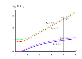
Figure 1: Equilibrium energy $\varepsilon_{\text{eq}}(T)$ (upper pair of curves) and entropy $s_{\text{eq}}(T)\$(lower pair of curves) for two different box sizes $L=1.0$ and $1.1$ obtained by using $p_{k,\text{eq}}(\beta,L)$. The point A on $L=1$ corresponds to $T=4.0$ for which the energy is $\varepsilon_{\text{eq}}\approx 2.7859$. The point B on $L=1.1$ has the same energy but has a higher temperature $T\approx 4.1728$.

Model We consider a gas of $N$ noninteracting identical structureless spin-free nonrelativistic particles, each of mass $m$, confined to a $1$-dimensional box with impenetrable walls and partitions, the latter dividing the box into different sizes. The box is isolated so that $d_{\text{e}}Q=0$. Initially, the gas is in thermodynamic equilibrium at temperature $T_{\text{i}}$ and pressure $P_{\text{i}}$ in state A${}_{\text{i,eq}}$, and is confined to a predetermined (such as the leftmost) small part of the box of length $L_{\text{i}}$ by the leftmost partition. At time $t=0$, the partition is instantaneously removed and the gas freely expands to a box of size $L=\alpha L_{\text{i}}$, $\alpha>1$, imposed by the next partition in a nonequilibrium fashion note2 . We wish to identify the instantaneous temperature and pressure of the gas as a function of the box size $L$.

Due to the lack of inter-particle interactions, we can focus on a single particle, an extensively studied model in the literature but with a very different emphasis Bender ; Doescher ; Stutz . Here, we study it from the current perspective. The particle only has non-degenerate eigenstates (standing waves) whose energies are determined by $L$ and a quantum number $k$; $p_{k}$ denotes their probabilities. We use the energy scale $\epsilon_{0}=\pi^{2}\hbar^{2}/2mL_{\text{i}}^{2}$ to measure the energy of the eigenstate so that $\varepsilon_{k}(L)=k^{2}/\alpha^{2}$; the corresponding eigenfunctions are given by

$$\psi_{k}(x)=\left\langle x\right|\left.k\right\rangle=\sqrt{2/L}\sin(k\pi x/L),\ k=1,2,\cdots.$$ (5)

The pressure in the $k$th eigenstate is given by $P_{k}(L)\equiv-\partial\varepsilon_{k}/\partial L=2\varepsilon_{k}(L)/L$ Landau-QM . The average energy and entropy per particle, and the pressure are given by (we suppress the $\left\{p_{k}\right\}$-dependence encoding all possible nonequilibrium states)

$$\varepsilon(L) \equiv{\textstyle\sum\nolimits_{k}}p_{k}\varepsilon_{k},s(L)\equiv-{\textstyle\sum\nolimits_{k}}p_{k}\ln p_{k}$$ (6a)

$$P(L) \equiv{\textstyle\sum\nolimits_{k}}p_{k}P_{k}=2\varepsilon(L)/L.$$ (6b)

The equilibrium state A${}_{\text{eq}}(T,L)$ at dimensionless temperature $T$ (in the units of $\epsilon_{0}$) is given by the Boltzmann law ($\beta\equiv 1/T$) for $p_{k}$:

$$p_{k\text{,eq}}(\beta,L)=\exp(-\beta\varepsilon_{k}(L))/Z_{0}(\beta,L);$$ (7)

$Z_{0}(\beta,L)\equiv{\textstyle\sum\nolimits_{k}}\exp(-\beta\varepsilon_{k}(L))$ is the partition function. The equilibrium macrostate is uniquely specified by $\{p_{k\text{,eq}}(\beta,L)\}$.

Results We plot $\varepsilon_{\text{eq}}(T,L)$ and $s_{\text{eq}}(T,L)$ in Fig. 1 as a function of $T$ for two different values of $L$; $P_{\text{eq}}=2\varepsilon_{\text{eq}}/L$. We observe that $\varepsilon$ decreases as $L$ increases. To study expansion in the isolated gas, for which $\varepsilon$ does not change Bender , we draw a horizontal line AB at $\varepsilon,$ which crosses the $L=1$ curve at $T_{1\text{eq}}$, and the $L=1.1$ curve at $T_{2\text{eq}}$. For $\varepsilon\simeq 2.7859$ (see below), $T_{1\text{eq}}=4.0$, and $T_{2\text{eq}}\simeq 4.1728$. As the gas expands isoenergetically from $L_{\text{i}}=1.0$ to $L=1.1$, its temperature varies from $T_{1\text{eq}}$ to eventually reach $T_{2\text{eq}}$ after the equilibration time $\tau_{\text{eq}}$. However, we learn something more from the figure. If we consider the temperature of the gas at some intermediate time $t$ during this period, such as immediately after the free expansion note2 , its temperature $T(t)$ will continuously change towards $T_{2\text{eq}}$ in time. The equilibrium entropy also increases with $L$ in an isothermal expansion, as expected; see the vertical line through A at $T=4.0$.

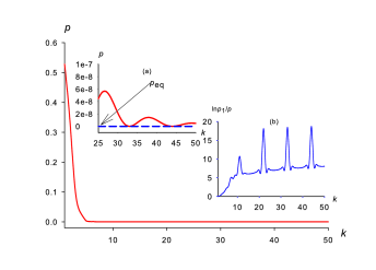
Figure 2: Eigenstate probabilities $p_{k}$ as a function of $k$ for $L=1.1$ after free expansion from state A₀. In the inset (a), we compare the equilibrium probabilities $p_{k\text{,eq}}$ for $L=1.1$ ($T=4.18$) and $p_{k}$ in the main frame for higher $k$’s that clearly show oscillations. In the inset (b), we plot $r\equiv\ln p_{1}/p_{k}$ that clearly shows oscillations even for small $k$’s; these oscillation are not present in $p_{k\text{,eq}}$. The curves in this figure are drawn for convenience.

To identify $T(t)$, we proceed in three steps. In the first step, we investigate the influence of quantum expansion on the entropy $s$. The gas is initially in a box of length $L_{\text{i}}$ with probabilities $p_{k_{\text{i}}}$ of eigenstates $\left|k_{\text{i}}\right\rangle\equiv\left|k,L_{\text{i}}\right\rangle$ and with energy and entropy per particle $\varepsilon_{\text{i}}$, and $s_{\text{i}}$, respectively. For an arbitrary state not in equilibrium or internal equilibrium, $p_{k}$ are independent of the energies $\varepsilon_{k}$ of the $k$th microstate. We find useful to deal with real probability ”amplitude” $a_{k}$ determining $p_{k}$ ($\equiv\left|a_{k}\right|^{2}$) in the following. The gas directly expands freely to a box of size $L_{1}$ or $L_{2}$, in each case starting from $L_{\text{i}}$, and we calculate the amplitudes of various eigenstates $\left|k_{\text{1}}\right\rangle\equiv\left|k,L_{\text{1}}\right\rangle$ and $\left|k_{\text{2}}\right\rangle\equiv\left|k,L_{\text{2}}\right\rangle$ in the two boxes:

$$a_{k_{1}}^{(\text{i})}=\sum_{k_{\text{i}}}a_{k_{\text{i}}}\left\langle k_{1}\right|\left.k_{\text{i}}\right\rangle,~{}a_{k_{2}}^{(\text{i})}=\sum_{k_{\text{i}}}a_{k_{\text{i}}}\left\langle k_{2}\right|\left.k_{\text{i}}\right\rangle,$$

from which we calculate the entropies $s_{1}^{(\text{i})}$ and $s_{2}^{(\text{i})}$, respectively; the superscript is a reminder of the memory effect since these quantities depend on the initial state through $p_{k_{\text{i}}}$. The coefficients $\left\langle k_{1}\right|\left.k_{\text{i}}\right\rangle$, etc. are Bender

$$\left\langle k_{1}\right|\left.k_{\text{i}}\right\rangle=\frac{2k_{\text{i}}\alpha^{3/2}(-1)^{k_{\text{i}}}}{\pi(k_{1}^{2}-\alpha^{2}k_{\text{i}}^{2})}\sin(\frac{k_{1}\pi}{\alpha}).$$

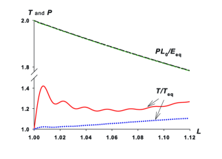
Figure 3: The normalized nonequilibrium temperature $T(L)/T_{\text{eq}}(L_{\text{i}})$ and pressure $P(L)L_{0}/\varepsilon_{\text{i}}(L_{\text{i}})$ for different $L$ after free expansion A${}_{\text{i}}\rightarrow$A$(L)$. We have taken $L_{\text{i}}=1.0$. The bottom two curves for $T(L)/T_{\text{eq}}(L_{0})$ correspond to $T_{\text{eq}}=1.0$ (solid) and $T_{\text{eq}}=4.0$ (dotted), respectively. The oscillations are more prominent at lower equilibrium temperatures but there is an overall tendency to increase. The two pressure curves for the two $T_{\text{eq}}$’s are almost indistinguishable on the scale of the plot and can be used as the ”exactness” of the computation. Theoretically, the normalized pressure is independent of the temperature.

Because of the ”deterministic” laws of quantum mechanics and the completeness of the eigenstates, the amplitude $\sum_{k_{1}}a_{k_{1}}^{(\text{i})}\left\langle k_{2}\right|\left.k_{1}\right\rangle$ of the eigenstate $\left|k_{2}\right\rangle$ after expansion from $L_{\text{i}}$ to $L_{1}$ to $L_{2}$ is exactly $a_{k_{2}}^{(\text{i})}$. Thus, the entropy $s_{2}^{(\text{i})}$ obtained from the direct expansion $L_{0}\rightarrow L_{2}$ is the same as the entropy obtained from the expansion sequence $L_{\text{i}}\rightarrow L_{1}\rightarrow L_{2}.$ We have also checked that the two entropies are the same to within our numerical accuracy in our computation. This means that the final ($L$) entropy has a memory of the initial ($L_{\text{i}}$) state, but not of the paths from $L_{\text{i}}$ to $L$. Thus, the entropy $s^{(\text{i})}(\varepsilon,L)$ in pure quantum mechanical evolution from a given initial state is not a state function of $\varepsilon$ and $L$. This is an important observation.

The memory effect results in a nonequilibrium state. The consequences of the latter can also be appreciated by considering the eigenstate probabilities $p_{k}$ for different $k$, which is shown in the main frame in Fig. 2 for $L=1.1$. It appears to fall off very rapidly, just as $p_{k\text{,eq}}$. However, while $p_{k\text{,eq}}$ monotonically decreases with $k$, $p_{k}$ has an oscillatory behavior, as shown in the inset (a) for $k$ between $25$ and $50$, where we compare the two probabilities; here, the former is effectively zero. The fine structure of this oscillatory behavior becomes obvious by considering the behavior of $\ln(p_{1}/p_{k})$, which is plotted in the inset (b) for $k\geq 1$. The oscillations are in conformity with the presence of sine in $\left\langle k_{1}\right|\left.k_{0}\right\rangle$, and should not be a surprise.

In the second step, we determine $T$ and $P$ for the nonequilibrium state A$(\varepsilon_{\text{i}},L)$ in a box of size $L$ after free expansion from $L_{\text{i}}$. The initial state A${}_{\text{i}}$ is an equilibrium state A${}_{\text{i,eq}}(T=4.0$ $(\varepsilon_{\text{i}}\approx 2.7859),L_{\text{i}}=1.0)$ for which $s_{\text{i,eq}}\approx 0.94$. The entropy difference $\Delta s\equiv s(L=1.1)-s_{\text{i,eq}}\approx 1.06-0.94=0.12$ is positive, which is expected in a free expansion. For the determination of the temperature, we proceed as follows. We allow the gas to freely expand ($P_{0}^{\prime}=0$) from $L$ by a ”differential” amount $dL\simeq 0.0000001$ to $L^{\prime}$. In this differential expansion, $dQ=d_{\text{i}}Q\equiv d_{\text{i}}W$ ($d_{\text{e}}Q=0$), and $d_{\text{i}}W=P(L)dL.$ We also compute the change in the entropy $ds\equiv$ $s(L^{\prime})-s(L)$. The ratio $PdL/ds$, see Eq. (2), determines the temperature $T$ of the nonequilibrium gas. For $L=1.1$, we determine the temperature to be $T(1.1)\approx 4.365$ using this differential method, which lies outside the equilibrium temperatures $T_{1\text{eq}}(1.0)=4.0$, and $T_{2\text{eq}}(1.1)=4.173$ quoted above. As we will show below, the higher nonequilibrium temperature is due to ”wider” microstate distribution relative to that for the equilibrium state. The results for $T(L)$ for different $L$ in the free expansion A${}_{\text{i,eq}}\rightarrow$A$(\varepsilon_{\text{i}},L)$ are shown in Fig. 3.

To add to the creditability of the above differential method for $T$, we apply it to determine $T$ for the equilibrium state A${}_{\text{i,eq}}(T=4.0,L=1.0)$. For such a state, the ratio $r=\ln(p_{1}/p_{k})L^{2}/(k^{2}-1)$ is $r=1/T$ for all $k$; see Eq. (7). As $p_{k,\text{eq}}$ falls exponentially with $k^{2}$, we truncate the number of microstates to $k\leq k_{\text{tr}}$ for which $p_{k,\text{eq}}\geq 10^{-15}$. This limits the number of microstates to $k\leq k_{\text{tr}}=$ $13$. If we truncate using $p_{k,\text{eq}}\geq 10^{-22}$, then we need to consider $k\leq k_{\text{tr}}=15$. Thus, truncating the number of microstates to $k_{\text{tr}}$ is computationally reasonable. The above calculation for the temperature with $k\leq k_{\text{tr}}=$ $13$ gives $T=4.00000$ to the first five decimal places, which adds to its creditability.

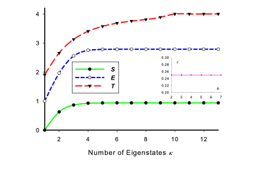
Figure 4: The effects of microstate numbers on the temperature, energy and entropy after heat exchange at constant $L$. The initial state is A${}_{\text{i,eq}}$. The curves are guides to the eye. In the inset, we plot the ratio $r\equiv\ln(p_{1}/p_{k})L^{2}/(k^{2}-1)$ for different microstates indexed by $k$ for the choice $\kappa=7$ in the main figure. The ratio is equal to the inverse temperature $1/4$ associated with A${}_{\text{i,eq}}(4.0)$, even though we have only seven microstates in the current state so that the truncated state cannot be identified with an equilibrium state at $T=4.0$.

We now ask the following question: What will happen if we consider only the first $\kappa$ microstates to determine the temperature, etc. by setting $p_{k,\text{eq}}=0$ for $k>\kappa$. Such truncated states are obviously not equilibrium states. To ensure that the probabilities add up to $1$, we normalize the probabilities, which does not affect the ratio $r$, as follows: $p_{k,\text{eq}}^{\prime}=p_{k,\text{eq}}/{\textstyle\sum}p_{k,\text{eq}}$. The results for the temperature, energy and entropy are shown in Fig. 4. In contrast, $r$ does not depend on the value of $\kappa$ as shown in the inset for $\kappa\leq 7$. But what we observe is an interesting phenomenon. As the number $\kappa$ increases, that is as the distribution gets ”wider,” the temperature gets higher and eventually gets to its limiting value of $4.0$.

The pressure is determined by Eq. (6b) by setting $\varepsilon(L)=\varepsilon_{\text{i}}$ so that $P(L)=2\varepsilon_{\text{i}}/L$. This is the statistical method (method 1) to compute $P(L)$. Accordingly, $P(L)$ in an isoenergetic process is a decreasing function of $L$. The ratio $P(L)L_{0}/\varepsilon_{\text{i}}$ is independent of the $T_{\text{i}}$ of the initial state, which is confirmed by our computation as shown by the upper curves for the two choices $T_{\text{i}}=1.0$ and $T_{\text{i}}=4.0$ in Fig. 3. There is another way (method 2) to determine the pressure in terms of the temperature, which is based on a thermodynamic relation: $P/T=(\partial s/\partial L)_{\varepsilon}$. We use the ratio of the ”differentials” $ds$ and $dL$ to determine $P/T$. We now use the statistical temperature in Fig. 3 in this ratio to compute the thermodynamic pressure $P$. The results are found to be indistinguishable from those shown in Fig. 3 by method 1, thus justifying our claim that the determination of our nonequilibrium temperature is meaningful as the ”internal” temperature of the system in that the two different methods to determine the pressure give almost identical values within our numerical accuracy.

As the memory of the initial state in $s_{1}^{(\text{i})},s_{2}^{(\text{i})},$ etc. cannot disappear by deterministic quantum evolution, some other mechanism is required for equilibration to come about in which the nonequilibrium entropy will gradually increase until it becomes equal to its equilibrium value. One possible mechanism based on the idea of ”chemical reaction” among microstates has been proposed earlier Gujrati-Entropy1 . We will consider the consequences of this approach elsewhere.

References

- (1) J. Keizer, J. Chem. Phys. 82, 2751 (1985).
- (2) W. Muschik, Aspects of non-equilibrium thermodynamics, World Scientific, Singapore (1990); see also W. Muschik and G. Brunk, Int. J. Engng Sci., 15, 377 (1977).
- (3) G.P. Morris and L. Rondoni, Phys. Rev. E 59, R5 (1999).
- (4) J. Casas-Vázquez and D. Jou, Rep. Prog. Phys. 66, 1937 (2003).
- (5) W.G. Hoover and C.G. Hoover, Phys. Rev. E 77, 041104 (2008).
- (6) D. Ruelle in Boltzmann’s Legacy, edited by G. Gallavotti, W. L. Reiter, and J. Yngvason, European Mathematical Society, Zürich, Switzerland (2008).
- (7) M. Planck in Festschrift Ludwig Boltzmann, p. 113, Barth, Leipzig (1904).
- (8) L.D. Landau, Zh. Eksp.Teor. Fiz. 7,203 (1937); Collected papers of L.D. Landau, p. 169, ed. D. ter Haar, Gordon and Breach, New York (1965).
- (9) W.H. Zurek, arXiv:quant-ph/0301076v1; see also W.H. Zurek in Frontiers of Nonequilibrium Statistical Physics, ed. GT Moore and MO Scully, Plenum, New York (1984).
- (10) R. Marathe and JMR Parrondo, Phys. Rev. Lett. 104, 245704 (2010).
- (11) S.W. Kim, T. Sagawa, S. De Libertato, and M. Ueda, Phys. Rev. Lett.106, 070401 (2011).
- (12) U. Siefert, Rep. Prog. Phys. 75, 126001 (2012).
- (13) N. Wiener, Cybernetics, or Control and Communication in the Animal and the Machine, John Wiley and Sons, New York (1948).
- (14) Brillouin, L., J. Appl. Phys. 22, 334 (1951).
- (15) K.L.C. Hunt, P.M. Hunt, and J. Ross, Annu. Rev. Phys. Chem.,41, 409 (1990).
- (16) K. Horn, M. Scheffler (Eds.), Handbook of Surface Science, vol. 2: Electronic Structure, Elsevier, Amsterdam (2000).
- (17) K. S. Førland, T. Førland, and S. Kjelstrup, Irreversible Thermodynamics: Theory and Application, Tapir, Trondheim, Norway, 3rd edition (2001).
- (18) P.D. Gujrati, Symmetry 2, 1201 (2010) and references therein.
- (19) P.D. Gujrati, Phys. Rev. E 81, 051130 (2010); P.D. Gujrati, arXiv:0910.0026.
- (20) P.D. Gujrati, Phys. Rev. E 85, 041128 (2012); P.D. Gujrati, arXiv:1101.0438.
- (21) P.D. Gujrati, Phys. Rev. E 85, 041129 (2012); P.D. Gujrati, arXiv:1101.0431.
- (22) P.D. Gujrati, arXiv:1105.5549.
- (23) P.D. Gujrati, arXiv:1304.3768.
- (24) P.D. Gujrati, Entropy, 17, 710 (2015).
- (25) L.D. Landau, E.M. Lifshitz, Statistical Physics, Vol. 1, Third Edition, Pergamon Press, Oxford (1986).
- (26) L.D. Landau, E.M. Lifshitz, Quantum Mechanics, Third Edition, Pergamon Press, Oxford (1977).
- (27) S.R. de Groot and P. Mazur, Nonequilibrium Thermodynamics, First Edition, Dover, New York (1984).
- (28) D. Kondepudi and I. Prigogine, Modern Thermodynamics, John Wiley and Sons, West Sussex (1998).
- (29) Following modern notation Prigogine ; deGroot , exchange of any extensive quantity with the medium and its change within the system carry the inner suffix e and i, respectively: . For example, we write and as the two components of the entropy change in a body: . A similar partition can also be made.
- (30) C.M. Bender, D.C. Brody and B.K. Meister, J. Phys. A 33, 4427 (2000), and Proc. Roy. Soc. A 461, 733 (2005).
- (31) S.W. Doescher and M.H. Rice, Am. J. Phys. 37, 1246 (1969).
- (32) D.W. Schlitt and C. Stutz, Am. J. Phys. 38, 70 (1970); C. Stutz and D.W. Schlitt, Phys. Rev. A 2, 897 (1970).
- (33) We neglect the time required for the eigenfunctions to expand to the new length, which is much smaller than .