Amplitude estimation of a sine function based on confidence intervals and Bayes’ theorem

Abstract

This paper discusses the amplitude estimation using data originating from a sine-like function as probability density function. If a simple least squares fit is used, a significant bias is observed if the amplitude is small compared to its error. It is shown that a proper treatment using the Feldman-Cousins algorithm of likelihood ratios allows one to construct improved confidence intervals. Using Bayes’ theorem a probability density function is derived for the amplitude. It is used in an application to show that it leads to better estimates compared to a simple least squares fit.

1 Introduction and motivation

This paper describes the amplitude estimation of a sine-like function. In general there is a bias towards an overestimation of the amplitude which is particularly significant if the amplitude is small compared to its error. Our starting point are data distributed on average according to the following functional form

$$y(x)\propto(1+A\sin(x)+B\cos(x))\,,$$ (1)

which can also be written as $(1+P\cos(x-\varphi))$ with $P=\sqrt{A^{2}+B^{2}}\geq 0$ and $\varphi=\mbox{atan2}(A,B)$ . Distributions like eq. (1) are widely discussed in signal processing [1, 2]. In particle physics they occur in scattering experiments with polarized beams and/or polarized targets. In this case $y(x)$ is proportional to the counting rate depending on the azimuthal angle $x$ [3], or, in case of a precessing polarization vector, $x$ is proportional to the time [4, 5]. Figure 1 (a) shows a distribution with $N=100$ events. The data were randomly generated according to eq. (1) with $A=0.1$ and $B=0$ and a Poisson statistical error was assumed. The black curve shows the result of a least squares fit.

The goal is to determine the amplitude $P=\sqrt{A^{2}+B^{2}}$. If $P$ is large, this is a trivial task by just performing a least squares fit. For $P$ close to the boundary $P=0$ the task is more difficult. For small amplitudes the estimated value $\hat{P}$ is on average larger than the true $P$. This is evident, because for $P=0$ the least squares fit in general results in $\hat{P}>0$. In the example of figure 1 (a) the fit yields $\hat{P}=0.20\pm 0.14$. As expected, the statistical error is approximately equal to $\sqrt{2/N}$. The exact expression for the error is derived in appendix A. Figure 1 (b) shows the result of $\hat{P}$ for 10000 fits to distributions generated with $P=0.1$. The average $\hat{P}$ amounts to 0.2 which corresponds to a bias of 0.1. Interpreting the fit result $\pm 1\,\sigma$ as a 68% confidence interval for $P$ may lead to coverage in the unphysical region below zero.

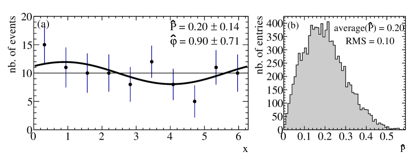
Figure 1: (a): Data points simulated according to eq. (1) with $N=100$ events with $A=0.1$ and $B=0$. The black line shows the result of a least squares fit with $\hat{P}=\sqrt{\hat{A}^{2}+\hat{B}^{2}}=0.20\pm 0.14$ and $\hat{\varphi}=0.90\pm 0.71$. (b): Distribution of $\hat{P}$ for $10000$ simulations.

The bias of the least squares estimate is discussed and given analytically in Refs. [1, 2]. However, in these references the question of unphysical values for the confidence interval is not addressed. The main subject of this paper is the application of the Feldman-Cousins algorithm [6] to construct proper confidence intervals for $P$ and deriving a probability density function for $P$ making use of Bayes’ theorem. Note that if the phase $\varphi$ is known, the distribution can be described by a single parameter $P$ where the estimated parameter $\hat{P}$ can be positive or negative although $P\geq 0$.

The paper is organized as follows. Section 2 describes the construction of confidence intervals. In section 3 a probability density function is derived. Section 4 discusses one application.

2 Construction of confidence intervals

For data distributed according to eq. (1), the probability distribution function for $\hat{P}=\sqrt{\hat{A}^{2}+\hat{B}^{2}}\geq 0$ can be derived analytically assuming that $\hat{A}$ and $\hat{B}$ are uncorrelated and normal distributed with means $A$ and $B$, respectively and variance $\sigma^{2}$. The combined distribution for $\hat{A}$ and $\hat{B}$ is given by

$$f(\hat{A}|A)f(\hat{B}|B)\mathrm{d}\hat{A}\mathrm{d}\hat{B} = \frac{1}{2\pi\sigma^{2}}\,\mathrm{e}^{-(\hat{A}-A)^{2}/(2\sigma^{2})}\mathrm{e}^{-(\hat{B}-B)^{2}/(2\sigma^{2})}\,\mathrm{d}\hat{A}\mathrm{d}\hat{B}\,.$$ (2)

The transformation to $\hat{P}=\sqrt{\hat{A}^{2}+\hat{B}^{2}}$ and $\hat{\varphi}=\mbox{atan2}(\hat{A},\hat{B})$ leads, after integration over $\varphi$, to

$$f(\hat{P}|P)\mathrm{d}\hat{P}=\frac{1}{\sigma^{2}}\,\mathrm{e}^{-(\hat{P}^{2}+P^{2})/(2\sigma^{2})}\hat{P}\,I_{0}\left(\frac{\hat{P}P}{\sigma^{2}}\right)\,\mathrm{d}\hat{P}$$ (3)

where $I_{0}$ is the modified Bessel function of first kind. Details are given in appendix B.

Figure 2 shows $f(\hat{P}|P)$ for $\sigma=\sqrt{2/100}$. It is known as the Rice distribution [7]. In figure 3 $f(\hat{P}|P)$ is shown for $P=0.4,0.1$ and $0$. For $P=0.4$ the estimated $\hat{P}$ follows approximately a normal distribution $N(P,\sigma)$. For smaller values of $P$ the bias $(\left<\hat{P}\right>-P)$ increases. In the case of $P=0.1$, one finds $\left<\hat{P}\right>=0.2$, which agrees well with the bias given in Refs. [2, 7] and with the observation in figure 1 (b). The magnitude of the bias depends not only on $P$ but also on $\sigma$.

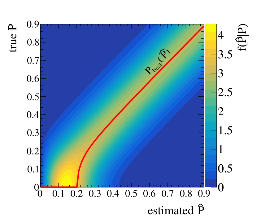
Figure 2: Probability density function $f(\hat{P}|P)$ for $\sigma=\sqrt{2/100}$. The red line shows $P_{\mathrm{best}}(\hat{P})$.

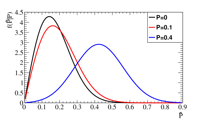
Figure 3: Probability density function $f(\hat{P}|P)$ for $P=0.4,0.1$ and $0$ for $\sigma=\sqrt{2/100}$.

In the following the Feldman-Cousins algorithm [6] is used to construct a confidence interval. A general introduction on confidence intervals can be found in ref. [8]. More details are also given in appendix C. At a given value of $P$ the algorithm selects all values of $\hat{P}$ for which the ratio

$$R(\hat{P},P)=\frac{f(\hat{P}|P)}{f(\hat{P}|P_{\mathrm{best}})}$$ (4)

has the largest values until the desired coverage of the confidence interval is reached. $P_{\mathrm{best}}$ denotes the value for which $f(\hat{P}|P_{\mathrm{best}})$ has its maximum in the allowed region of $P$, i.e. $f(\hat{P}|P_{\mathrm{best}})=\max\{f(\hat{P}|P)\}$. $P_{\mathrm{best}}$ as a function of $\hat{P}$ is shown in figure 2 as a red line.

Figure 4 shows the 68% (blue) and 90% (gray) confidence intervals for $N=100$ (a) and $N=1000$ events (b). In the case of $N=100$ and a measured value $\hat{P}=0.1$ the 68% confidence interval for $P$ ranges from 0 to 0.14. At larger values of $\hat{P}$ the 68% confidence interval coincides with the Gaussian error expectation $\left[P-\sqrt{2/N},P+\sqrt{2/N}\right]$. For larger $N$, the transition to a Gaussian confidence interval occurs at smaller values of $P$. By construction, the confidence intervals only contain values in the physical region $P\geq 0$.

3 Derivation of probability density function

The previous section described how a confidence interval can be defined for $P$ given a measured $\hat{P}$. If the amplitude $P$ is the final result of the experiment, this is sufficient. However, in many applications $P$ is used as an input in a subsequent analysis. In this case, it is desirable to have a probability density function (pdf) for $P$. Unfortunately, it is not directly possible to construct such a pdf without further assumptions. To proceed, we make use of the Bayes’ theorem with a constant prior probability for $P$. This leads to the following pdf:

$$\tilde{f}(P|\hat{P})=\frac{f(\hat{P}|P)}{\int_{0}^{\infty}f(\hat{P}|P)\mathrm{d}P}\,.$$

Note that $\tilde{f}(P|\hat{P})\propto R(\hat{P},P)$ for a fixed $\hat{P}$. In case of $\hat{P}=0.1$ and $\sigma=\sqrt{2/100}$ the interval $[0,0.16]$ covers 68%, i.e. $\int_{0}^{0.16}\tilde{f}(P|\hat{P})\mathrm{d}P=0.68$. For comparison, the corresponding Feldman-Cousins interval is $[0,0.14]$. In the next section an application is discussed where we will make use of this pdf.

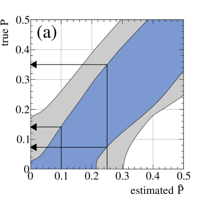
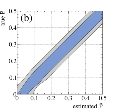
Figure 4: Confidence intervals for 68% (blue) and 90% (gray) coverage for $N=100$ events (a) and $N=1000$ events (b). In figure (a) for a measured $\hat{P}=0.1(0.25)$ the 68% confidence interval for $P$ is $[0,0.14]\,([0.073,0.35])$ as indicated by the arrows.

4 Application

We study the case where the amplitude decays exponentially with time. In figure 5 the dotted line shows an exponential function $C\mbox{e}^{-t/\tau}$ with a decay constant $\tau=1$ and amplitude $C=0.3$. Data were generated at ten different times $t$ following the distribution $f(\hat{P}|P)$ in eq. (3) with $P=C\mbox{e}^{-t/\tau}$, $\sigma=\sqrt{2/N}$ and $N=1000$. These values are displayed as data points. The blue curve shows the result of a least squares fit to these data points. The vertical bands at each $t$-bin show the pdf $\tilde{f}(P|\hat{P})$ as a function of $P$, where $\hat{P}$ is the generated value (i.e. the data point). The red curve shows the result of a likelihood fit with the likelihood function

$$\mathcal{L}=\Pi_{i=1}^{N_{bin}}\,\,\tilde{f}(C\mbox{e}^{-t_{i}/\tau}|P_{i})$$

varying $\tau$ and $C$ to maximize $\mathcal{L}$. In this example the likelihood fit yields 1.20$\pm$0.37 (red line) for $\hat{\tau}$ compared to 1.81 $\pm$ 0.51 (blue line) for the least squares fit to the black points. Figure 6 shows the result of 10000 simulations. The average of $\hat{\tau}$ is 1.04 for the likelihood and 1.63 for the least squares fit. On average the likelihood result has a bias of 0.04/0.35=0.11 of its statistical error, whereas the bias for the least square fit is 0.63/0.48=1.3. This proves that the likelihood fit using $\tilde{f}(\hat{P}|P)$ as a pdf gives a result closer to the true value $\tau=1$. Since the likelihood method is only asymptotically unbiased ($N_{\mathrm{bin}}\rightarrow\infty$), the small bias even decreases if the number of $t$-bins is increased.

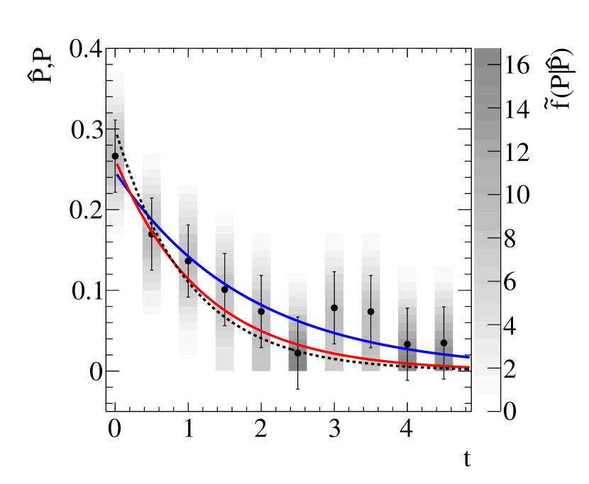
Figure 5: Dotted line: $P(t)=C\mbox{e}^{-t/\tau}$ with $\tau=1$ and $C=0.3$. Data points: random values according to $f(\hat{P}|P(t_{i})),\quad i=1,\dots,10$ with $\sigma=\sqrt{2/1000}$. Blue line: result of a least squares fit to the data points. Vertical bands: probability distribution $\tilde{f}(P|\hat{P})$ for true $P$ for the given generated $\hat{P}$. Red line: Result of a likelihood fit to these probability distributions.

Figure 6: Distribution of $\hat{\tau}$ for 10000 simulations. Results from likelihood fit using the probability distributions (a), and a least squares fit (b).

5 Conclusions

Parameter estimations play an important role in all area of science. Estimates of theses parameters obtained from least squares fits assuming Gaussian errors are often biased even for simple scenarios like the estimation of an amplitude of a sine-function. This may in addition introduce coverage in non-physical regions of the parameter.

In this paper we made use of the Feldman-Cousins algorithm to construct confidence intervals for the amplitude $P$ of a sine-function covering only the allowed region $P\geq 0$. Further, a probability density function (pdf) for the amplitude was derived applying the Bayes’ theorem. In an application it was shown that using this pdf leads to better fit results compared to a simple least squares fit.

Appendix A Statistical error of amplitude and phase

Starting from the probability density function

$$y(x)=(1+P\cos(x-\varphi))\,,\quad 0\leq x<2\pi\,,$$

the log-likelihood function reads

$$\ell=\sum_{i=1}^{N}\log(1+P\cos(x_{i}-\varphi))\,.$$

Using the second derivatives

$$\frac{\partial^{2}\ell}{\partial P^{2}} = -\sum_{i}\frac{\cos^{2}(x-\varphi)}{(1+P\cos(x-\varphi))^{2}}\,,$$ (5)

$$\frac{\partial^{2}\ell}{\partial\varphi^{2}} = -\sum_{i}\frac{-P^{2}\sin^{2}(x-\varphi)}{(1+P\cos(x-\varphi))^{2}}\,,$$ (6)

$$\frac{\partial^{2}\ell}{\partial P\partial\varphi} = -\sum_{i}\frac{\sin(x-\varphi)}{(1+P\cos(x-\varphi))^{2}}\,$$ (7)

and their expectation values

$$\left<\frac{\partial^{2}\ell}{\partial P^{2}}\right> = N\,\int_{0}^{2\pi}\frac{\partial^{2}\ell}{\partial P^{2}}(x)\,y(x)\mathrm{d}x$$

$$= N\,\frac{1-\sqrt{1/(1-P^{2})}}{P^{2}}\stackrel{{\scriptstyle P^{2}\ll 1}}{{\approx}}-\frac{N}{2}\left(1+\frac{3}{4}P^{2}\right)\,,$$

$$\left<\frac{\partial^{2}\ell}{\partial\varphi^{2}}\right> = N\,\frac{1-\sqrt{1/(1-P^{2})}}{\sqrt{1/(1-P^{2})}}\stackrel{{\scriptstyle P^{2}\ll 1}}{{\approx}}-\frac{NP^{2}}{2}\,,$$

$$\left<\frac{\partial^{2}\ell}{\partial P\partial\varphi}\right> = 0\,.$$

the errors on $P$ and $\varphi$ can be calculated. To $\mathcal{O}(P^{2})$ they are given by

$$\sigma_{P}^{-2} = \frac{N}{2}\left(1+\frac{3}{4}P^{2}\right)\,,$$

$$\sigma_{\varphi}^{-2} = \frac{NP^{2}}{2}\,.$$

Note that for a sufficient large number of bins the errors derived here for the unbinned likelihood method coincide with the errors of the least squares fit.

Appendix B Derivation of the Rice distribution

Starting from eq. (2)

$$f(\hat{A}|B)f(\hat{B}|B)\mathrm{d}\hat{A}\mathrm{d}\hat{B} = \frac{1}{2\pi\sigma^{2}}\,\mathrm{e}^{-(\hat{A}-A)^{2}/(2\sigma^{2})}\mathrm{e}^{-(\hat{B}-B)^{2}/(2\sigma^{2})}\,\mathrm{d}\hat{A}\,\mathrm{d}\hat{B}\,,$$ (8)

the transformation to $\hat{P}$ and $\hat{\varphi}$ yields

$$f(\hat{P},\hat{\varphi}|P,\varphi)\,\mathrm{d}\hat{P}\,\mathrm{d}\hat{\varphi} = \frac{1}{2\pi\sigma^{2}}\,\mathrm{e}^{-(\hat{P}\sin\hat{\varphi}-P\sin\varphi)^{2}/(2\sigma^{2})}\mathrm{e}^{-(\hat{P}\cos\hat{\varphi}-P\cos\varphi)^{2}/(2\sigma^{2})}\,\hat{P}\mathrm{d}\hat{P}\mathrm{d}\hat{\varphi}\,$$ (10)

$$\frac{1}{2\pi\sigma^{2}}\,\mathrm{e}^{-(\hat{P}^{2}+P^{2})/(2\sigma^{2})}\mathrm{e}^{-(2\hat{P}P(\sin\varphi\sin\hat{\varphi}+\sin\varphi\sin\hat{\varphi})/(2\sigma^{2})}\,\hat{P}\mathrm{d}\,\hat{P}\,\mathrm{d}\hat{\varphi}\,$$

Using

$$\int_{0}^{2\pi}\mbox{e}^{(2P\hat{P}(\sin(\varphi)\sin(\hat{\varphi})+\cos(\varphi)\cos(\hat{\varphi}))/(2/\sigma^{2})}\mathrm{d}\hat{\varphi}=2\pi I_{0}\left(\frac{P\hat{P}}{\sigma^{2}}\right)$$ (11)

the integration over $\hat{\varphi}$ results in

$$f(\hat{P}|P)=\frac{1}{\sigma^{2}}\,\mathrm{e}^{-(\hat{P}^{2}+P^{2})/(2\sigma^{2})}\,I_{0}\left(\frac{P\hat{P}}{\sigma^{2}}\right)\,\hat{P}\,.$$ (12)

$I_{0}$ is the modified Bessel function of first kind.

Appendix C Details of the Feldman-Cousins confidence interval construction

This appendix shows how confidence intervals are constructed in practice. The starting point is the likelihood ratio $R(\hat{P},P)$ (eq. (4)) shown in figure 7. For each value of true $P$ a lower and upper limit of $\hat{P}$ is obtained in the following way. For a given $P$ one starts at the largest value of $R$ (see figure 8 (a) for $P=0.1$). All values of $\hat{P}$ are included in the interval until the desired coverage is reached (see figure 8 (b)). In the example given in figure 8 the 68% interval $[\hat{P}_{\mathrm{min}},\hat{P}_{\mathrm{max}}]$ is $[0.07,0.27]$ and the 90% interval is $[0,0.34]$. Repeating this procedure for all values of $P$ yields the boundary lines of the colored areas in figure 4. This construction makes no use of the measured value.

Given a measurement $\hat{P}$ the confidence interval for $P$ is given by the two values on the $y$-axis where the vertical line starting at $\hat{P}$ intersects the boundary lines. This is indicated in Fig. 4 (a) for $\hat{P}=0.1$ and $\hat{P}=0.25$ for the 68% intervals.

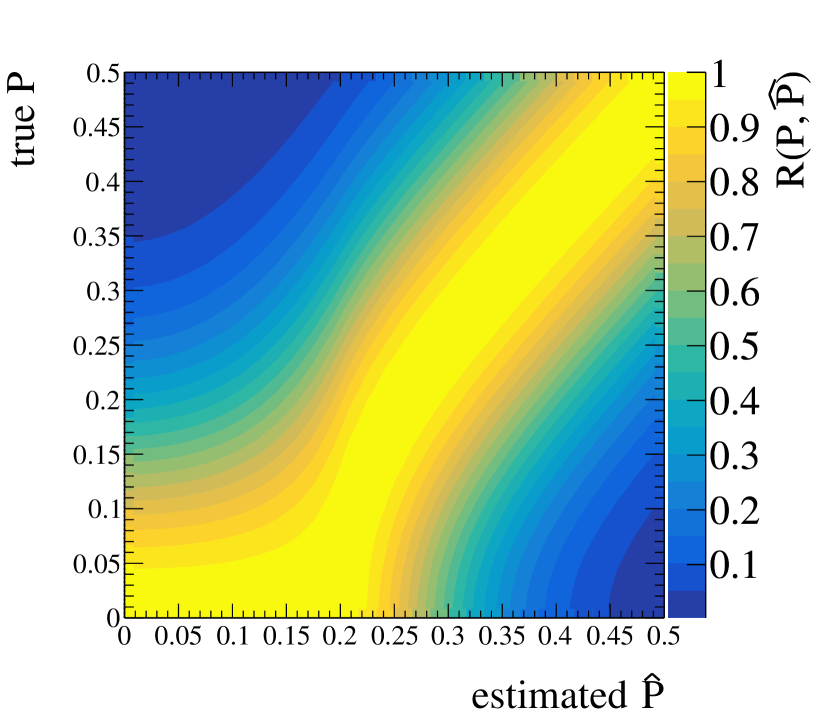
Figure 7: The likelihood ratio $R(\hat{P},P)$ for $\sigma=\sqrt{2/100}$.

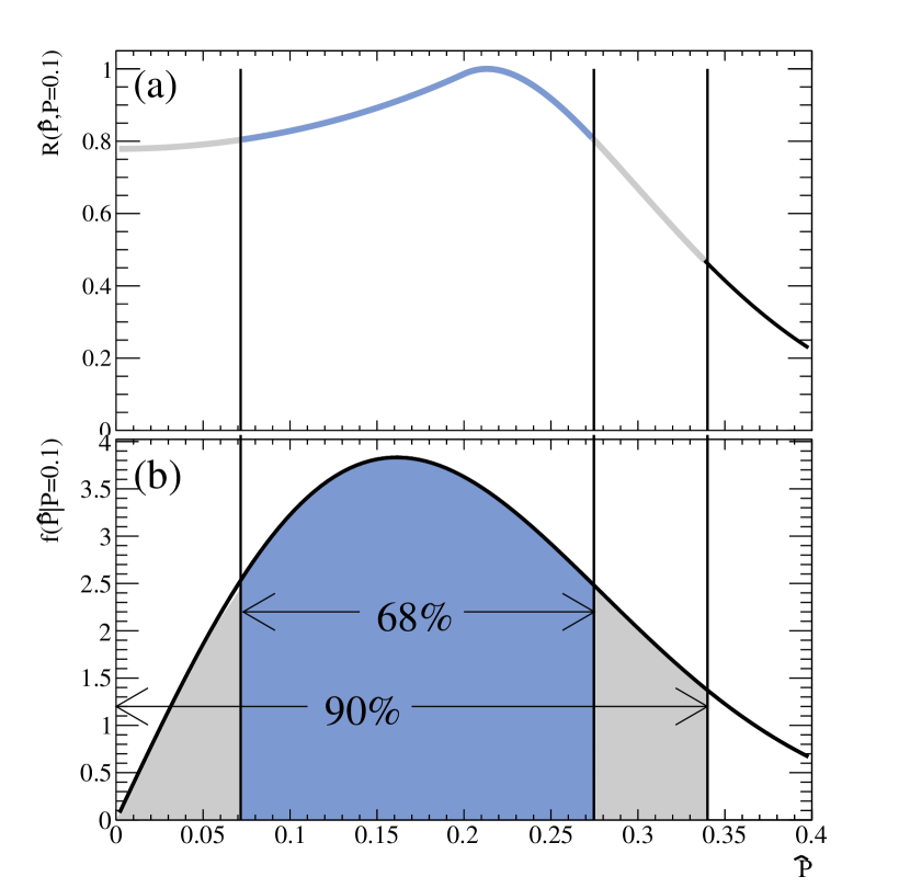
Figure 8: Construction of confidence interval. (a): The likelihood ratio $R(\hat{P},P=0.1)$ (see eq. (4)). (b):The probability density function $f(\hat{P}|P=0.1)$ for $\sigma=\sqrt{2/100}$. Starting from the largest value of $R$ in the upper plot all values of $\hat{P}$ are included until the desired confidence interval is reached.

References

[1]
F. C. Alegria, “Bias of amplitude estimation using three-parameter sine
fitting in the presence of additive noise,” Measurement, vol. 43,
pp. 766–770, 2010.
[2]
P. Händel, “Amplitude estimation using IEEE-STD-1057 three-parameter sine
wave fit: Statistical distribution, bias and variance,” Measurement,
vol. 42, pp. 748–756, 2009.
[3]
B. v. Przewoski et al., “Analyzing powers and spin correlation
coefficients for elastic scattering at 135 and 200 MeV,” Phys.
Rev. C, vol. 74, p. 064003, Dec 2006.
[4]
D. Eversmann et al., “New method for a continuous determination of the
spin tune in storage rings and implications for precision experiments,”
Phys. Rev. Lett., vol. 115, no. 9, p. 094801, 2015.
[5]
Z. Bagdasarian et al., “Measuring the polarization of a rapidly
precessing deuteron beam,” Phys. Rev. ST Accel. Beams, vol. 17,
p. 052803, May 2014.
[6]
G. J. Feldman and R. D. Cousins, “A Unified approach to the classical
statistical analysis of small signals,” Phys. Rev., vol. D57,
pp. 3873–3889, 1998.
[7]
P. Peebles, Probability, Random Variables And Random Signal Principles.
McGraw-Hill higher education, McGraw-Hill Education (India) Pvt
Limited, 2002.
[8]
F. James, Statistical Methods in Experimental Physics.
World Scientific Publishing, 2006.