Quantum correlations and coherence between two particles interacting with a thermal bath

Abstract

Quantum correlations and coherence generated between two free spinless particles in the lattice, interacting with a common quantum phonon bath are studied. The reduced density matrix has been solved in the Markov approach. We show that the bath induces correlations between the particles. The coherence induced by the bath is studied calculating: off-diagonal elements of the density matrix, spatiotemporal dispersion, purity, and quantum mutual information. We have found a characteristic time-scale pointing out when this coherence is maximum. In addition a Wigner-like distribution in the phase-space (lattice) has been introduced as an indirect indicator of the quantumness of total correlations and coherence induced by the thermal bath. The negative volume of the Wigner function shows also a behavior which is in agreement with the time-scale that we have found. A Gaussian distribution for the profile of particles is not obtained and interference pattern are observed as the result of bath induced coherence. As the temperature of bath vanishes the ballistic behavior of the tight-binding model is recovered. The geometric quantum discord has been calculated to characterize the nature of the correlations.

Keywords: Dissipative Quantum Walks, Quantum decoherence, Quantum correlation.

1 Introduction

In quantum systems, damping and fluctuations enter through the coupling with an external large bath $\mathcal{B}$. The conventional treatment computes the reduced density matrix of the system, $\mathcal{S}$, by expanding in the coupling strength to the bath and eliminating these variables. Nevertheless, some extra approximations must be introduced to arrive to a completely positive map [1]. This conclusion can be summarized in the appropriated structure that the Quantum Master Equation (QME) must have after the elimination of bath. In fact, this QME is known to be acceptable only for few particular cases [2, 3, 4, 5, 6].

Here we study a minimal model that indeed leads to a well defined QME (completely positive infinitesimal semigroup), then we can compute analytically several quantum measures. In this way we can show that a thermal bath generates not only dissipation, but indeed induces coherence and non-classical correlations between particles immersed in it [7]. In an analogous way, total correlations generated between a Spin $\frac{1}{2}$ (the system) and the Magnet apparatus (pointer variable) coupled to a boson thermal bath show that correlations develop in time, reach a maximum, then disappear later and later [5]. Other similar works have been proposed to show bath-generated correlations in a system, induced from a thermal common bath [7].

In order to study bath-induced correlations, we present exact calculations on the dynamics of spinless Quantum Walks (QWs) [8, 9, 10]. As expected, quantum measures will vanish as time goes on due to the dissipation. Then, the important point would be to characterize when these induced correlations and coherences start to decrease. We will present analytical calculations of these measures and also we compute the characteristic time-scale when they are maxima before being wiped out by the dissipation. As an indirect measure of the quantum character of the state of the system, the negative volume of the Wigner function and the quantum coherence from off-diagonal elements of the density matrix –as a function of time– have also been studied.

There are several measures to get information concerning quantum correlations, in particular, we will focus on the quantum discord [11]. As we mentioned before, our system presents coherence and non-classical correlations, in particular, we can indirectly measure the nonclassical correlation by calculating the geometric quantum discord, which in fact is an accepted measure despite its criticisms [12]. Then we can use these results to measure the quantum to classical transition, for example, in qubit systems [13, 14, 15].

The simplest implementations that reflect the role of a coherent superposition can be proposed in the framework of QW experiments, or its numerical simulations [16, 17, 18, 19, 20, 21]. A Dissipative QW (DQW) has also been defined as a spinless particle moving in a lattice and interacting with a phonon bath [9, 22, 23]. In particular in this work we will implement explicit calculations for a system $\mathcal{S}$ constituted by two distinguishable particles in a one-dimensional regular lattice. The present approach can also be extended to tackle the many-body fermionic particles (or bosonic, see appendix A); then, pointing out the interplay between particle-particle and bath-particle interactions.

2 Dissipative Quantum Walks

The goal of this section is not intended to derive the completely positive infinitesimal generator, this section is presented to show explicitly the contribution responsible of the bath-induced coherence in the system, see appendix B. Here we introduce shift operators that define the model of two free distinguishable spinless particles (system $\mathcal{S})$ coupled to a common phonon bath $\mathcal{B}$. The generalization to bosonic or fermionic particles can be done in a similar way using Fock’s representation, see appendix A.

The total Hamiltonian for $\mathcal{S}$ coupled to a common bath $\mathcal{B}$ can be written using the Wannier basis in the following way (for more details see [9, 23]). Let the total Hamiltonian be

$$H_{\mathcal{T}}=H_{\mathcal{S}}+H_{\mathcal{B}}+H_{\mathcal{SB}}.$$ (1)

$H_{\mathcal{S}}$ is the free tight-binding Hamiltonian (our system $\mathcal{S}$)

$$H_{\mathcal{S}}=2E_{0}\mathbf{I}-\frac{\Omega}{2}\left(a_{12}^{{\dagger}}+a_{12}\right),$$ (2)

here $\{a_{12}^{{\dagger}},a_{12}\}$ are shift operators for the particles labeled $1$ and $2$, and $\mathbf{I}$ the identity in the Wannier basis

$$\mathbf{I}=\sum_{s,s^{{}^{\prime}}}\arrowvert s,s^{{}^{\prime}}\rangle\langle s,s^{{}^{\prime}}\arrowvert$$

$$a_{12}^{{\dagger}}\arrowvert s_{j},s_{l}\rangle=\arrowvert s_{j}+1,s_{l}\rangle+\arrowvert s_{j},s_{l}+1\rangle$$ (3)

$$a_{12}\arrowvert s_{j},s_{l}\rangle=\arrowvert s_{j}-1,s_{l}\rangle+\arrowvert s_{j},s_{l}-1\rangle.$$ (4)

Note that a “shift operator” translates each particle individually. Here we have used a “pair-ordered” bra-ket $\arrowvert s_{j},s_{l}\rangle$ representing the particle “$1$” at site $s_{j}$ and particle “$2$” at site $s_{l}$; note that these operators generate the free tight-binding Hamiltonian (2), see Appendix A. From Eqs. (3)-(4) it is simple to see that

$$\left[a_{12}^{{\dagger}},a_{12}\right]=0,$$ (5)

and also that

$$a_{12}a_{12}^{{\dagger}}\arrowvert s_{j},s_{l}\rangle\!=\!2\arrowvert s_{j},s_{l}\rangle+\arrowvert s_{j}-1,s_{l}+1\rangle+\arrowvert s_{j}+1,s_{l}-1\rangle.$$ (6)

$H_{\mathcal{B}}$ is the phonon bath $H_{\mathcal{B}}=\sum\limits_{k}\hbar\omega_{k}\mathcal{B}_{k}^{{}^{{\dagger}}}\mathcal{B}_{k}$, thus $\{\mathcal{B}_{k}^{{}^{{\dagger}}},\mathcal{B}_{k}\}$ are bosonic operator characterizing the thermal bath in equilibrium. In eq. (1) the term $H_{\mathcal{SB}}$ is the interaction Hamiltonian between $\mathcal{S}$ and $\mathcal{B}$,

$$H_{\mathcal{SB}}=\hbar\Gamma\left(a_{12}\otimes\sum\limits_{k}v_{k}\mathcal{B}_{k}+a_{12}^{{\dagger}}\otimes\sum\limits_{k}v_{k}^{\ast}\mathcal{B}_{k}^{{}^{{\dagger}}}\right),$$ (7)

where $v_{k}$ represents the spectral function of the phonon bath, and $\Gamma$ is the interaction parameter in the model. This is a minimal interacting model useful for our purposed study. Getting the QME from this interaction model produces clearly two separable contributions, this fact will be studied in detail in the next sections.

To study a non-equilibrium evolution for the system $\mathcal{S}$, we calculate from (1) –eliminating the bath variables– a dissipative quantum infinitesimal generator (see appendix A in [24]). Therefore, tracing out bath variables, and in the Ohmic approximation, we can write the Markov Quantum Master Equation (QME) [1, 5, 23]:

$$\frac{d\rho}{dt}\! = \!\frac{-i}{\hbar}\left[H_{eff},\rho\right]+\frac{D}{2}\left(2a_{12}\rho a_{12}^{{\dagger}}-a_{12}^{{\dagger}}a_{12}\rho-\rho a_{12}a_{12}^{{\dagger}}\right)$$ (8)

$$+ \frac{D}{2}\left(2a_{12}^{{\dagger}}\rho a_{12}-a_{12}a_{12}^{{\dagger}}\rho-\rho a_{12}^{{\dagger}}a_{12}\right),$$

where $D\equiv\Gamma^{2}k_{B}T/\hbar$, here $T$ is the temperature of the bath $\mathcal{B}$. We point out that due to the particular interaction Hamiltonian model $H_{\mathcal{SB}}$ that we have used, it is possible to see that the algebra is closed for the operators of $\mathcal{S}$, then we can prove the QME is a bonafide semigroup [6]. Adding $-2E_{0}+\Omega$ to $H_{\mathcal{T}}$ the effective Hamiltonian turns to be

$$H_{eff}=\Omega\left(\mathbf{I}-\frac{a_{12}^{{\dagger}}+a_{12}}{2}\right)-\hbar\omega_{c}a_{12}a_{12}^{{\dagger}},$$

where $\omega_{c}$ is the frequency cut off in the Ohmic approximation. This Hamiltonian is the natural extension of van Kampen’s Hamiltonian for two spinless particles in the lattice [9, 24].

From the QME (8) we can see that the term

$$\frac{-D}{2}\left(a_{12}^{{\dagger}}a_{12}\rho+\rho a_{12}a_{12}^{{\dagger}}+a_{12}a_{12}^{{\dagger}}\rho+\rho a_{12}^{{\dagger}}a_{12}\right),$$ (9)

is the responsible of generating coherence in the system (see appendix B), the structure of this operator can be realized from the analysis of operators like $a_{12}a_{12}^{{\dagger}}$, see (6). While the decoherence of the system comes from the term

$$\frac{D}{2}\left(2a_{12}\rho a_{12}^{{\dagger}}+2a_{12}^{{\dagger}}\rho a_{12}\right),$$

and its interpretation can be done just in terms of one-step translation of particles (see appendix A in Fock’s representation).

Here we will focus in the highly dissipative regime so we can take $\omega_{c}=0$ without lost of generality. It can be seen from Eq.(8) that as $D\rightarrow 0$ the unitary evolution is recovered (the tight-binding model). The limit $D\rightarrow\infty$ (or $\Omega\rightarrow 0$) corresponds to the case when the effective Hamiltonian disappears, then we would expect a pure random dynamics corresponding to two Random Walk (RW). Nevertheless, for the quantum two-body problem that we are working, the classical profile, even when $D/\hbar\Omega\gg 1$, cannot be reached because coherence have been induced from bath $\mathcal{B}$.

We will solve this QME (8) using a localized Initial Condition (IC) in the Wannier lattice, i.e.,:

$$\rho(t=0)=\arrowvert 0,0\rangle\langle 0,0\arrowvert\equiv\arrowvert\vec{0}\rangle\langle\vec{0}\arrowvert.$$ (10)

The operational calculus in the QME will be done using a two-particles Wannier vector state to evaluate elements of the density matrix $\rho(t)$.

3 The Two-Body Solution of QME

Using (3)-(6) the QME (8) can be worked out. In particular to find the analytical solution of $\rho(t)$ is it simpler to do the calculations in Fourier representation. Then we introduce here the two-particle Fourier basis (similar calculus where done for the one-particle problem [23, 24, 14, 15]). The Fourier ”bra-ket” is defined in terms of the two particles Wannier basis in the form:

$$\left|k_{1},k_{2}\right\rangle=\frac{1}{2\pi}\sum\limits_{s_{1},s_{2}\in\mathcal{Z}}e^{ik_{1}s_{1}}e^{ik_{2}s_{2}}\left|s_{1},s_{2}\right\rangle,$$ (11)

here $\mathcal{Z}$ is the set of integer numbers. Thus Eq.(8) for two particles can be written as:

$$\frac{d}{dt}\!\left\langle k_{1},\!k_{2}\left|\rho\left(t\right)\right|k_{1}^{\prime},\!k_{2}^{\prime}\right\rangle\!=\!\mathcal{F}(k_{1},\!k_{1}^{\prime},\!k_{2},\!k_{2}^{\prime})\!\!\left\langle k_{1},k_{2}\left|\rho\left(t\right)\right|k_{1}^{\prime},k_{2}^{\prime}\right\rangle.$$ (12)

Using the IC (10) and the braket (11) the solution in Fourier basis is

$$\left\langle k_{1},k_{2}\left|\rho\left(t\right)\right|k_{1}^{\prime},k_{2}^{\prime}\right\rangle=e^{\mathcal{F}(k_{1},k_{1}^{\prime},k_{2},k_{2}^{\prime})t},$$ (13)

where

$$\mathcal{F}(k_{1},k_{1}^{\prime},k_{2},k_{2}^{\prime}) \equiv \left[\mathcal{F}^{(1)}(k_{1},k_{1}^{\prime})+\mathcal{F}^{(1)}(k_{2},k_{2}^{\prime})\right]$$ (14)

$$+ 2D[\mathbf{C}\left(k_{1}\!,k_{2}^{\prime}\right)+\mathbf{C}\left(k_{2}\!,k_{1}^{\prime}\right)$$

$$- \mathbf{C}\left(k_{1}\!,k_{2}\right)-\mathbf{C}\left(k_{1}^{\prime}\!,k_{2}^{\prime}\right)].$$

We note that

$$\mathcal{F}^{(1)}(k_{i},k_{i}^{\prime})\equiv\left[\!\frac{-i}{\hbar}\!\left(\mathcal{E}_{k_{i}}\!-\!\mathcal{E}_{k_{i}^{\prime}}\right)\!+\!2D\!\left(\mathbf{C}\left(k_{i}\!,k_{i}^{\prime}\right)-\!1\right)\!\right],$$ (15)

is the one-particle infinitesimal generator in the Fourier representation where

$$\mathcal{E}_{k_{i}}\equiv\Omega\left\{1-\cos k_{i}\right\},$$ (16)

that is, the eigenenergy of the free particle labeled ”$i$” in the lattice [24]. The function

$$\mathbf{C}\left(k\!_{1},k_{2}\right)\equiv\cos\left(k_{1}-\!k_{2}\right)\!,$$ (17)

takes into account the interaction induced between the particles. Therefore the second term in (14) represents the interaction between particles mediated by the thermal bath. In order to get insight into the mathematical meaning of this interaction we can solve a pseudo infinitesimal generator considering only the interaction term: $2D[\mathbf{C}\left(k_{1}\!,k_{2}^{\prime}\right)+\mathbf{C}\left(k_{2}\!,k_{1}^{\prime}\right)-\mathbf{C}\left(k_{1}\!,k_{2}\right)-\mathbf{C}\left(k_{1}^{\prime}\!,k_{2}^{\prime}\right)]$, that comes from (9). In this case the solution will be normalized, but the eigenvalues are not necessarily positive. This contribution in the full infinitesimal generator (14) is the responsible of cross-terms producing coherence between the two-particles, see appendix B.

If we solve (12) with $D=0$ the solution will represent two free tight-binding particles in the lattice (i.e., a unitary evolution). If we solve (12) with $\Omega=0$ and neglect the mentioned interaction, this case will represent a classical problem (two RWs). In addition, from (12) the result: $\langle k_{1},k_{2}|d\rho(t)/dt|k_{1},k_{2}\rangle=0$ says that the diagonal Fourier elements are constant in time (i.e., a momentum-like conservation law). In the section V using the Wigner function, we will comment this statement.

The elements of $\rho(t)$ can be calculated on the Wannier basis, then we can write an analytical formula for $\rho(t)$ in the real lattice: $\langle s_{1},s_{2}|\rho(t)|s_{1,}^{\prime}s_{2}^{\prime}\rangle$.

Using

$$\arrowvert s_{1},s_{2}\rangle=\frac{1}{2\pi}\int_{-\pi}^{\pi}\int_{-\pi}^{\pi}dk_{1}dk_{2}\ e^{-ik_{1}s_{1}}e^{-ik_{2}s_{2}}\arrowvert k_{1},k_{2}\rangle,$$

in the general solution of the QME (13), we get $\!\rho(t)$ in Wannier’s basis

$$\left\langle s_{1},s_{2}\left|\!\rho(t)\!\right|s_{1}^{\prime},s_{2}^{\prime}\right\rangle\! = \!\frac{1}{\left(2\pi\right)^{4}}\!\int\int\int\int\limits_{-\pi}^{+\pi}\prod\limits_{i=1}^{2}dk_{i}\!\!\ dk_{i}^{\prime}\!\!\ e^{ik_{1}s_{1}-ik_{1}^{\prime}s_{1}^{\prime}}$$ (18)

$$\times e^{ik_{2}s_{2}-ik_{2}^{\prime}s_{2}^{\prime}}e^{\mathcal{F}\left(k_{1},k_{1}^{\prime},k_{2},k_{2}^{\prime}\right)t},$$

$$\quad\{s_{j},s_{l}^{\prime}\}\in\emph{Z}.$$

These integrals can be done analytically considering Bessel’s properties:

$$e^{iz\cos\theta}=\sum_{n=-\infty}^{\infty}i^{n}J_{n}(z)e^{in\theta};\;\;e^{z\cos\theta}=\sum_{n=-\infty}^{\infty}I_{n}(z)e^{in\theta},$$

where $J_{n}$ and $I_{n}$ are Bessel’s functions of integer order $n\in\mathcal{Z}$. These functions satisfies that [25]

$$J_{-n}(x)=(-1)^{n}J_{n}(x),\ J_{n}(-x)=(-1)^{n}J_{n}(x),$$

and

$$I_{-n}(x)=I_{n}(x),\ I_{n}(-x)=(-1)^{n}I_{n}(x).$$

Then, we can write finally a closed expression for $\langle s_{1},s_{2}|\rho(t)|s_{1,}^{\prime}s_{2}^{\prime}\rangle$.

To simplify the notation we use $t_{\Omega}\equiv\frac{\Omega t}{\hbar},t_{D}\equiv 2Dt$ whenever it is necessary, then

$$\langle s_{1},s_{2}|\rho(t)|s_{1}^{\prime},s_{2}^{\prime}\rangle\! = \!i^{(s_{1}-s_{1}^{\prime}+s_{2}-s_{2}^{\prime})}e^{-2t_{D}}\!\!\!\!\!\!\!\!\!\!\!\!\!\!\!\!\!\!\!\!\sum_{\{n_{1},n_{2},n_{3},n_{4},n_{5},n_{6}\}\in\mathcal{Z}}\!\!\!\!\!\!\!\!\!\!\!\!\!\!\!\!(-1)^{n_{4}+n_{5}}\$$ (19)

$$\times J_{s_{1}+n_{1}+n_{2}+n_{5}}\!\!\left(t_{\Omega}\right)\!\!\ J_{s_{1}^{\prime}+n_{1}+n_{3}+n_{4}}\!\!\left(t_{\Omega}\right)$$

$$\times \!\!J_{s_{2}+n_{3}-n_{5}+n_{6}}\!\!\left(t_{\Omega}\right)\!\!\ J_{s_{2}^{\prime}+n_{2}-n_{4}+n_{6}}\!\!\left(t_{\Omega}\right)\!\!$$

$$\times \prod\limits_{n_{i}=1}^{6}I_{n_{i}}\!\left(t_{D}\right),\ \{s_{j},s_{l}^{\prime}\}\in\mathcal{Z}.$$

This solution is symmetric under the exchange of particles (i.e., preserving the symmetry of the IC). Of course, $\rho(t)$ is Hermitian, positive definite and satisfies normalization in the lattice, that is:

$$\langle s_{1},s_{2}|\rho(t)|s_{1}^{\prime},s_{2}^{\prime}\rangle\! = \!\langle s_{1}^{\prime},s_{2}^{\prime}|\rho^{\ast}(t)|s_{1},s_{2}\rangle,\ \{s_{1},s_{2}\}\in\mathcal{Z}$$

$$\mbox{Tr}[\rho(t)] = \!\!\!\!\sum_{\{s_{1},s_{2}\}\in\mathcal{Z}}\langle s_{1},s_{2}|\rho(t)|s_{1},s_{2}\rangle=1,\forall t,$$

the last line can be proved using Bessel’s properties:

$$\sum_{n=-\infty}^{\infty}I_{n+m}(x)I_{n}(x) = I_{m}(2x)$$ (21)

$$\sum_{n=-\infty}^{\infty}(-1)^{n}I_{n+m}(x)I_{n}(x) = \delta_{m,0}.$$ (22)

The fact that $\rho(t)$ is positive definite, for all $t\geq 0$, follows from the structural theorem when it is applied to our bonafide semigroup (8) [1].

The probability of finding one particle in site $s_{1}$ and another in $s_{2}$ is given by probability profile:

$$P_{s_{1},s_{2}}(t)\equiv\langle s_{1},s_{2}|\rho(t)|s_{1},s_{2}\rangle,$$

and shows for the present IC (10) the expected reflection symmetry in the plane: $s_{1}-s_{2}=0$.

Equation (19) contains all the information concerning the bath-induced correlations (off-diagonal elements). Note that $H_{\mathcal{S}}$ in (2) represents free distinguishable particles, the particle-particle correlations are bath induced from (9).

In the case $D=0$, i.e., a closed system without dissipation, we recover the density matrix for two QWs (the tight-binding solution):

$$\langle s_{1},s_{2}|\rho(t)|s_{1}^{\prime},s_{2}^{\prime}\rangle_{D=0}=\prod_{j=1}^{j=2}i^{(s_{j}-s_{j}^{\prime})}J_{s_{j}}\!\left(t_{\Omega}\right)\!J_{s_{j}^{\prime}}\!\left(t_{\Omega}\right).$$

This means that for a localized IC and in a closed system, $\rho(t)$ can be written for any time $t>0$ as direct product of two independent particles, i.e., $\rho(t)=\rho_{1}(t)\otimes\rho_{2}(t)$ .

Interestingly, in the case $D\rightarrow\infty$ (or $\Omega\rightarrow 0$) the classical regimen (two RWs) is not recovered [26, 27] because $\mathcal{B}$ has created quantum coherence between them. Thus, in the case $D\gg\Omega/\hbar$ the solution $\rho(t)$ is not the direct product of two particles $\rho(t)\neq\rho_{1}(t)\otimes\rho_{2}(t)$,

$$\langle s_{1},s_{2}|\rho(t)|s_{1}^{\prime},s_{2}^{\prime}\rangle_{\Omega=0}\! = \!(-1)^{(s_{1}+s_{1}^{\prime})}\delta_{s_{1}+s_{2},s_{1}^{\prime}+s_{2}^{\prime}}\ e^{-2t_{D}}$$

$$\times \!\!\!\!\!\!\!\!\sum_{\{n_{1},n_{2},n_{3}\}\in\mathcal{Z}}\!\!\!\!\!\!(-1)^{n_{1}+n_{2}}\!\ I_{s_{1}+n_{1}+n_{3}}\!\left(t_{D}\right)$$

$$\times \!\!I_{-s_{2}+n_{2}+n_{3}}\!\left(t_{D}\right)\!\ I_{n_{1}}\!\left(t_{D}\right)\!\ I_{n_{2}}\!\left(t_{D}\right)$$

$$\times \!\!I_{s_{1}-s_{1}^{\prime}+n_{1}+n_{2}+n_{3}}\!\left(t_{D}\right)\!\ I_{n_{3}}\!\left(t_{D}\right).$$

Then, showing a complex pattern structure in terms of convolutions of classical profiles.

From Eq.(3) we note that when $D\gg 1$ we get the probability profile:

$$P_{s_{1},s_{2}}(D\gg 1)\! \neq \!P_{s_{1}}(D\gg 1)\!\times\!P_{s_{2}}(D\gg 1)=e^{-4Dt}\$$

$$\times \!\!I_{s_{1}}\!\left(2Dt\right)\!I_{s_{2}}\!\left(2Dt\right),$$

here $P_{s_{j}}$ is the classical probability for each particle $j=1,2$ in the sites $s_{1}$ and $s_{2}$ respectively. This result explicitly shows that in the asymptotic regime $t\rightarrow\infty$ the classical profile is not obtained. Thus the profile of probability for two DQW will not be a Gaussian distribution. As we have commented before this is so because of off-diagonal elements in $\rho(t)$ have been generated by the evolution of the QME (quantum coherence bath induced).

We note that due to the presence of the bath there is a competition between dissipation and building up coherence. This issue will be analyzed using different measures in the next subsections.

3.1 Change of basis for $\rho\left(t\right)$ for two DWQs

An outstanding conclusion can be observed by introducing a change of basis $U_{a}^{\dagger}\rho(t)U_{a}$ in the representation of the two-particle density matrix. Which in fact is a function of parameters $(D,\Omega)$ and the time $t$, see Eq.(19).

Among several possibilities, and in order to calculate eigenvalues rather than the eigenvectors, here we define a (dynamic) change of basis using a time-dependent unitary transformation $U_{a}$ characterized by the elements

$$\langle s_{1},s_{2}\arrowvert U_{a}\arrowvert s_{1}^{\prime},s_{2}^{\prime}\rangle=i^{\left(s_{1}+s_{2}+s_{1}^{\prime}+s_{2}^{\prime}\right)}J_{s_{1}-s_{1}^{\prime}}(\!\frac{\Omega t}{\hbar})J_{s_{2}-s_{2}^{\prime}}(\!\frac{\Omega t}{\hbar}),$$ (24)

with

$$\langle s_{1},s_{2}\arrowvert U_{a}U_{a}^{\dagger}\arrowvert s_{1}^{\prime},s_{2}^{\prime}\rangle=\delta_{s_{1},s_{1}^{\prime}}\delta_{s_{2},s_{2}^{\prime}}.$$ (25)

Then, considering as before the IC $\rho(t=0)=\arrowvert 0,0\rangle\langle 0,0\arrowvert$, it can be proved that

$$\langle s_{1},\!s_{2}\arrowvert U_{a}^{\dagger}\rho(t)U_{a}\arrowvert s_{1}^{\prime},\!s_{2}^{\prime}\rangle\! = \!\!\!\sum_{s_{1}^{{}^{\prime\prime}},s_{2}^{{}^{\prime\prime}}}\sum_{s_{1}^{{}^{\prime\prime\prime}},s_{2}^{{}^{\prime\prime\prime}}}\langle s_{1},s_{2}\arrowvert U_{a}^{\dagger}\arrowvert s_{1}^{\prime\prime},s_{2}^{\prime\prime}\rangle$$

$$\times \langle s_{1}^{\prime\prime},s_{2}^{\prime\prime}\arrowvert\rho(t)\arrowvert s_{1}^{\prime\prime\prime},s_{2}^{\prime\prime\prime}\rangle$$

$$\times \langle s_{1}^{\prime\prime\prime},s_{2}^{\prime\prime\prime}\arrowvert U_{a}\arrowvert s_{1}^{\prime},s_{2}^{\prime}\rangle$$

$$= \delta_{s_{1}+s_{2},s_{1}^{\prime}+s_{2}^{\prime}}\ \left(-1\right)^{s_{2}^{\prime}-s_{2}}\ e^{-2t_{D}}$$

$$\times \sum_{n_{1},n_{2},n_{5}}\left(-1\right)^{n_{2}+n_{5}}\ I_{n_{2}}\!(t_{D}\!)$$

$$\times \!\!I_{n_{3}}\!(t_{D}\!)I_{n_{5}}\!(t_{D}\!)I_{n_{2}+n_{5}+s_{1}}\!(t_{D}\!)$$

$$\times \!\!I_{n_{3}+n_{5}-s_{2}}\!(t_{D}\!)I_{n_{2}+n_{5}+n_{3}+s_{2}^{\prime}-s_{2}}\!(t_{D}\!),$$

in the last equality we have used Bessel’s identity $\sum_{s}J_{s+m}(\!x)J_{s+p}(\!x)=\delta_{m,p}$. Comparing (3.1) with (3) we can conclude that in this new representation

$$\tilde{\rho}(t)\equiv U_{a}^{\dagger}\rho(t)U_{a}=\rho(\Omega=0,D,t),$$ (27)

i.e., $\tilde{\rho}(t)$ does not depend on the tigth-binding energy $\Omega$. Then, it is simple to see that the new $\tilde{\rho}(t)$ is Hermitian and equal to the highly dissipative case, and of course normalized to one. In addition, it can be proved that purity and entropy are invariant under this unitary transformation [28].

This is an interesting result because allows us to study many quantum properties using a simplest expression for the density matrix instead of carrying on the analysis with the two parameters $(D,\Omega)$. Properties as purity, entropy, etc., can straightforwardly be understood in this new representation. We note that using $U_{a}$, eigenvectors also will change, then a partial trace would be affected by this map. But in the present paper, we do not calculate any partial trace using $U_{a}$.

3.2 Reduced Density Matrix for One Particle.

At this point it is interesting to calculate from the full expression Eq.(19), the reduced density matrix for one particle. This analysis will help to understand the model and ultimately the induced coherence in the system. To do this we trace out over the degrees of freedom of one particle, say $j=2$. Then, the reduced density matrix for one particle is obtained as

$$\langle s_{1}|\rho^{(1)}(t)|s_{1}^{\prime}\rangle\!=\!\langle s_{1}\arrowvert\mbox{Tr}_{2}[\rho(t)]\arrowvert s_{1}^{\prime}\rangle\!=\!\sum_{s_{2}\in\mathcal{Z}}\langle s_{1},s_{2}|\rho(t)|s_{1}^{\prime},s_{2}\rangle.$$ (28)

Alternatively, note that using the Fourier expression Eq.(18) it is straightforward to find that

$$\langle s_{1}|\rho^{(1)}(t)|s_{1}^{\prime}\rangle\!=\!\!\left(2\pi\right)^{-2}\!\!\!\int\!\!\!\!\int\!\!dk_{1}\!\!\ dk_{1}^{\prime}\!\!\ e^{ik_{1}s_{1}-ik_{1}^{\prime}s_{1}^{\prime}}e^{\mathcal{F}^{(1)}\left(k_{1},k_{1}^{\prime}\right)t},$$

with $\mathcal{F}^{(1)}(k_{1},k_{1}^{\prime})\!\!=\!\!\{\!\frac{-i}{\hbar}\!\left(\mathcal{E}_{k_{1}}\!-\!\mathcal{E}_{k_{1}^{\prime}}\right)\!+\!2D\!\left(\cos\left(k_{1}\!-\!k_{1}^{\prime}\right)\!-\!1\right)\!\}$, the one-particle infinite generator. Then, we arrive to the result

$$\langle s_{1}|\rho^{(1)}\!(t)|s_{1}^{\prime}\rangle\!\!=\!i^{(s_{1}-s_{1}^{\prime})}e^{-t_{D}}\!\!\!\sum_{n\in\mathcal{Z}}\!\!J_{s_{1}+n}\!\left(t_{\Omega}\right)\!\!\ J_{s_{1}^{\prime}+n}\!\left(t_{\Omega}\right)\!\!\ I_{n}\!\left(t_{D}\right)\!.$$ (29)

This marginal solution corresponds to the one-particle density matrix with IC $\rho(t=0)=\arrowvert 0\rangle\langle 0\arrowvert$, and shows when $D\gg\Omega/\hbar$ asymptotically the same behavior than a classical RW [24]. A result that is not entirely surprising because in the Hamiltonian (1) each particle is originally non-interacting between them. We remain that the correlations are built up between the particles as a result of the interaction with $\mathcal{B}$. In the next section we will show that the two-body profile does not behave as two classical random walks in any asymptotic regime.

3.3 Eigenvalues of $\rho(t)$

Here we calculate the eigenvalues of the density matrix for any fixed time. In the case of one-particle the expression for the eigenvalues is analytical. On the other hand, in the two-particles case, numerical calculations can be done using our exact result written in terms of Bessel’s functions.

3.3.1 The one-body reduced density matrix case

Consider the solution of the one-particle reduced density matrix (29). We want to find a new representation where $\rho^{(1)}(t)\!$ is diagonal for any fixed time $t$; that is, we want to find a unitary transformation $U$ such that

$$U^{\dagger}\rho^{(1)}U=\tilde{\rho}^{(1)}.$$

Thus, using the solution (29) we can explicitly show (where $t_{D}=2Dt,t_{\Omega}\equiv\Omega t/\hbar$) that

$$\left(U^{\dagger}\rho^{(1)}U\right)_{nk} = \langle n|U^{\dagger}\rho^{(1)}U|k\rangle=\sum_{r,q}\left(U^{\dagger}\right)_{nr}\rho_{rq}^{(1)}U_{qk}$$ (30)

$$= \!e^{-t_{D}}\!\!\sum_{r,q}\left(U^{\dagger}\right)_{nr}U_{qk}\ i^{(r-q)}\!\!\sum_{\alpha\in\mathcal{Z}}\!J_{r+\alpha}\!\left(t_{\Omega}\right)$$

$$\times J_{q+\alpha}\!\left(t_{\Omega}\right)\!\!\ I_{\alpha}\!\left(t_{D}\right)$$

$$= e^{-t_{D}}\sum_{\alpha\in\mathcal{Z}}I_{\alpha}\!\left(t_{D}\right)\sum_{r}i^{r}U_{rn}^{\ast}\ J_{r+\alpha}\!\left(t_{\Omega}\right)$$

$$\times \sum_{q}i^{-q}U_{qk}\ J_{q+\alpha}\!\left(t_{\Omega}\right)\!\!\ .$$

Noting that $\sum_{n=-\infty}^{\infty}J_{r+n}(x)J_{r+\alpha}(x)=\delta_{n,\alpha}$, we see from (30) that if

$$U_{qk}=i^{(q+k)}J_{q+k}\left(t_{\Omega}\right),$$ (31)

we get $U^{\dagger}U=\mathbf{1}$ (unitary transformation), then

$$\left(U^{\dagger}\rho^{(1)}U\right)_{nk} = e^{-t_{D}}\sum_{\alpha\in\mathcal{Z}}I_{\alpha}\!\left(t_{D}\right)\ i^{k-n}\delta_{n,\alpha}\delta_{k,\alpha}$$ (32)

$$= e^{-t_{D}}I_{n}\!\left(t_{D}\right)\ \delta_{n,k}$$

This means that the eigenvalues and their normalized eigenvectors are

$$\lambda_{0} = e^{-t_{D}}I_{0}\!\left(t_{D}\right)\ \;\;\rightarrow\;(\cdots,i^{k}J_{k}\left(t_{\Omega}\right),\cdots)^{T},$$

$$\lambda_{\pm 1} = e^{-t_{D}}I_{\pm 1}\!\left(t_{D}\right)\ \rightarrow\;(\cdots,i^{\pm 1+k}J_{\pm 1+k}\left(t_{\Omega}\right),\cdots)^{T},$$

$$\lambda_{\pm 2} = e^{-t_{D}}I_{\pm 2}\!\left(t_{D}\right)\rightarrow\;(\cdots,i^{\pm 2+k}J_{\pm 2+k}\left(t_{\Omega}\right),\cdots)^{T},$$ (33)

$$\mbox{with}\;\;k\in 0,\pm 1,\pm 2,\cdots\;\;\;\mbox{etc.}$$

We note that $\lambda_{n}\in\mathcal{R}_{e}\ (\forall n\in 0,\pm 1,\pm 2,\cdots)$ and that they are bounded in the interval $1\geq\lambda_{n}\geq 0.$

In figure 1 we show the eigenvalues $\lambda_{n}$ of the $1$-body reduced density matrix $\rho^{(1)}\left(t\right)$ for $t_{D}=2Dt=4$. The inset in this figure shows the plot of the numerical calculation ordered from the largest one. We can see that the eigenvalues are degenerate in pairs, except for the first eigenvalue. This fact can be understood as follows: by means of the unitary transformation (31) we can write $\rho\left(t\right)\$in a diagonal form using the eigenvalues (33)

$$\tilde{\rho} = \sum_{n=-\infty}^{+\infty}\lambda_{n}\arrowvert n\rangle\langle n\arrowvert$$

$$= \sum_{n=-\infty}^{-1}\lambda_{n}\arrowvert n\rangle\langle n\arrowvert+\sum_{n=1}^{+\infty}\lambda_{n}\arrowvert n\rangle\langle n\arrowvert+\lambda_{0}\arrowvert 0\rangle\langle 0\arrowvert$$

$$= \sum_{n=1}^{+\infty}\lambda_{n}\arrowvert n\rangle\langle n\arrowvert+\sum_{n=1}^{+\infty}\lambda_{-n}\arrowvert-n\rangle\langle-n\arrowvert+\lambda_{0}\arrowvert 0\rangle\langle 0\arrowvert,$$

then, we conclude that $\tilde{\rho}$, with the IC (10), is invariant under reflection symmetry $\arrowvert n\rangle\rightarrow\arrowvert-n\rangle$, and so the eigenvalues $\lambda_{n}$ are degenerate in pairs $\lambda_{n}=\lambda_{-n}$ except $\lambda_{0}$ as it is shown in figure 1.

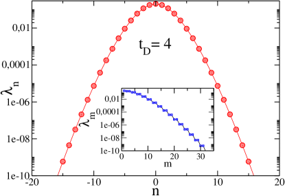
Figure 1: (Color online) Analytical eigenvalues (in log scale) of the one-body reduced density matrix. The inset shows the numerical calculation ordered from the largest eigenvalue.

Also from (31) we see that the density matrix is normalized:

$$\mbox{Tr}\left[\tilde{\rho}\right]=\sum_{n\in\mathcal{Z}}\lambda_{n}=\sum_{n\in\mathcal{Z}}e^{-t_{D}}I_{n}\!\left(t_{D}\right)=1.$$ (34)

Using this new basis we can write an analytical expression for the one-particle purity and entropy (they are invariant under unitary transformations [28]). In this basis

$$\left(\tilde{\rho}^{(1)}\right)^{2}\! = \!\left(\sum_{n\in\mathcal{Z}}\lambda_{n}\arrowvert n\rangle\langle n\arrowvert\right)^{2}\!=\!\sum_{n,m\in\mathcal{Z}}\lambda_{n}\lambda_{m}\arrowvert n\rangle\langle n\arrowvert m\rangle\langle m\arrowvert$$ (35)

$$= \sum_{n\in\mathcal{Z}}\lambda_{n}^{2}\arrowvert n\rangle\langle n\arrowvert,$$

therefore, using (21), the purity is

$$\mathcal{P}_{Q}^{(1)}\left(t\right)=\mbox{Tr}\left[\left(\tilde{\rho}^{(1)}\right)^{2}\right] = \sum_{n\in\mathcal{Z}}e^{-2t_{D}}\ \left[I_{n}\!\left(t_{D}\right)\right]^{2}$$ (36)

$$= e^{-2t_{D}}I_{0}\!\left(2t_{D}\right).$$

In an analog way the entropy can also be calculated analytically

$$S^{(1)}\!\! = \!\!-\mbox{Tr}\left[\tilde{\rho}^{(1)}\ln\tilde{\rho}^{(1)}\right]$$ (37)

$$= \!\!-\!\!\sum_{n\in\mathcal{Z}}\lambda_{n}\ln\lambda_{n}\!\!=\!-\!\!\sum_{n\in\mathcal{Z}}e^{-t_{D}}I_{n}\!\left(t_{D}\right)\ln\left(e^{-t_{D}}I_{n}\!\left(t_{D}\right)\right)$$

$$= -\sum_{n\in\mathcal{Z}}e^{-t_{D}}I_{n}\!\left(t_{D}\right)\left[-t_{D}+\ln\left(I_{n}\!\left(t_{D}\right)\right)\right]$$

$$= t_{D}-e^{-t_{D}}\sum_{n\in\mathcal{Z}}I_{n}\!\left(t_{D}\right)\ln\left(I_{n}\!\left(t_{D}\right)\right),$$

where we have used (33).

To end this section we comment that (37) agrees with numerical calculations presented in [24] ($S^{(1)}$ is linear for $t_{D}<<1$). In particular when $D=0$ and noting that $I_{n}\!\left(0\right)=\delta_{n,0}$ we get that $S^{(1)}=0$, and in general for $D\neq 0$ we get $S^{(1)}\left(t\right)>0,$ $\forall t>0.$

3.3.2 The two-body density matrix case

Consider the two-particle density matrix (19). Here we want to find the eigenvalues of $\rho(t)\!$ for any fixed time $t$. Using the unitary transformation $U_{a}$ presented in (24) the two-particle density matrix can be written in the form $\tilde{\rho}(t)\equiv\rho(\Omega=0,D,t)$, as was proved in (27). Unfortunately, we were not able to find an analytical expression for these eigenvalues in the case of two particles, but its analysis can be done numerically from $\tilde{\rho}(t)$. In figure 2 we show the eigenvalues of the two-body density matrix $\tilde{\rho}(t)$ for $t_{D}=2Dt=4$. Comparing this figure with the inset of figure 1, it can be realized the complex structure for the two-body eigenvalues. It can be seen that there are degenerated eigenvalues in pairs, and also non-degenerated values (see figure 2). In order to understand these degererancy we have carried out a numerical analysis of eigenvectors. Then, we can conclude that the symmetry that is behind the two-particles eigenvalue is also the refection symmetry of the two-particle eigenvector. That is, consider the Wannier ket $\arrowvert s_{i},s_{j}\rangle$ and the symmetry $s_{i}+s_{j}=n$, a two-particle eigenvector can be written in the form:

$$\arrowvert c_{1},c_{2}\rangle=b\arrowvert s_{1},s_{2}\rangle+b^{\prime}\arrowvert s_{1}^{\prime},s_{2}^{\prime}\rangle+\cdots,$$

such that

$$s_{1}+s_{2}=n,\ s_{1}^{\prime}+s_{2}^{\prime}=n,\cdots,\ \mbox{with }n=1,2,\cdots,$$

and its corresponding eigenvalue is degenerated with the case$\ m=-1,-2,\cdots$. The non-degenerated eigenvalues correspond to eigenvectors in the subspace with $s_{i}+s_{j}=0$. It means that $\tilde{\rho}\left(t\right)$ is diagonalizable in blocks with $s_{1}+s_{2}=s_{1}^{\prime}+s_{2}^{\prime}=\cdots$.

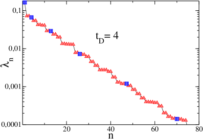
Figure 2: (Color online) Eigenvalues of the two-body (reduced) density matrix. The squares represent the non-degenerated eigenvalues.

4 Quantum coherence

To study the coherence we will use standard measures to characterize the process. Among the different measures, here we present the ones that allow us analytical results: Profile probability, von Neuman entropy, Purity, Quantum coherence, and Spatiotemporal dispersion. Non-classical correlations and the negativity of the Wigner function will we presented in separated sections.

4.1 Purity

To see the influence of $\mathcal{B}$ to build up coherence between the particles, we calculate the quantum purity $\mathcal{P}_{Q}(t)\equiv\mbox{Tr}[\rho(t)^{2}]$. Linear entropy or impurity of the system $\mathcal{S}_{L}=1-\mathcal{P}_{Q}$ is a lower approximation to the quantum von Neuman entropy $-\mbox{Tr}[\rho\ln\rho]$, then if system remains pure ($\mathcal{P}_{Q}=1$) or mixed ($\mathcal{P}_{Q}<1$). In our case we can study analytically this two-body quantity in the course of time:

$$\mathcal{P}_{Q}^{(2)}(t)\!=\!\!\!\!\!\!\! e^{-4t_{D}}\sum_{m\in\mathcal{Z}}I_{m}\left(2t_{D}\right)\sum_{\{\alpha,\beta\}\in\mathcal{Z}}(-1)^{\alpha+\beta}I_{\alpha}\left(2t_{D}\right)$$

$$\times \!I_{\beta}\left(2t_{D}\right)I_{\alpha+m}\left(2t_{D}\right)I_{\beta+m}\left(2t_{D}\right)I_{\alpha+\beta+m}\left(2t_{D}\right).$$

It can be seen for $D=0$ (without dissipation) that purity $\mathcal{P}_{Q}^{(2)}(t)$ takes the value one for all time. But for the case $D\neq 0$ the purity is lower than one and decreases in time. For $D\neq 0$ the purity is different from the purity for two-particles with independent quantum bath, i.e.,

$$\mathcal{P}_{Q}^{(2)}(t)\neq\mathcal{P}_{Q}^{(1)}(t)\mathcal{P}_{Q}^{(1)}(t),$$

here $\mathcal{P}_{Q}^{(1)}(t)$ is the corresponding one-particle purity with independent bath $\mathcal{P}_{Q}^{(1)}(t)=e^{-2t_{D}}I_{0}\left(2t_{D}\right)$ [24]. Therefore a common quantum bath $\mathcal{B}$ has produced a difference $\Delta\mathcal{P}_{Q}=\mathcal{P}_{Q}^{(2)}(t)-\mathcal{P}_{Q}^{(1)}(t)\mathcal{P}_{Q}^{(1)}(t)$ which shows the occurrence of classical and non-classical correlations between particles.

The purity $\mathcal{P}_{Q}$ is related to the entropy $S(t)$ of the system. In figure 3(a) we show that $\rho(t)$ for two particles with a common bath has more purity than in the case of two particles with independent baths. This fact can be thought as a measure of the bath induced coherence between the particles. The inset in figure 3(a) shows the difference of the purity $\Delta\mathcal{P}_{Q}$ between the two mentioned cases, showing that $\Delta\mathcal{P}_{Q}$ has in fact a maximum of coherence and then decreases slowly. Therefore, for $t_{D}^{\max}=2Dt^{\max}\sim 1$ there is a characteristic time-scale before the effect of dissipation wipe out the coherence induced by the bath. This result will be compared in the next sections with the coherence measured from the off-diagonal elements of the two-body density matrix, and the negative volume of the Wigner function.

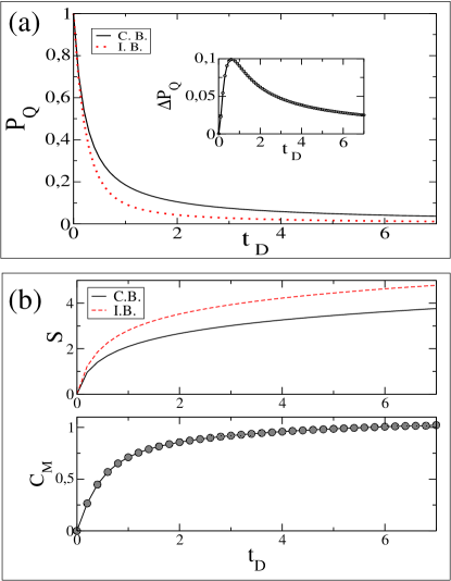
Figure 3: (Color online) (a) Purity from a localized IC (10) as function of $t_{D}=2Dt$. Plots in straight lines are for the case with a common bath, dashed lines are with independent baths. The inset shows the difference of the Purity between the cases: two DQWs with a common $\mathcal{B}$ (C.B.), and two DQWs with independent baths (I.B.).
(b) Entropy for a localized IC (10) as function of $t_{D}=2Dt$, for two different cases. Plots in straight line is for the case of two particles with a common bath, dashed line is with independent baths. In the bottom the QMI ($C_{M}$) is shown as a function of $t_{D}$.

The figure 3(b) the entropy and the Quantum Mutual Information (QMI) are also plotted as a function of $t_{D}$. On the top of this figure the entropy is shown for two particles with common bath $S^{\left(12\right)}(t)$ and independent baths $2S^{\left(1\right)}(t)$. In the bottom of this figure, we plot $C_{M}(t)$ which quantify the QMI:

$$C_{M}(t)=S^{\left(1\right)}(t)+S^{\left(2\right)}(t)-S^{\left(12\right)}(t)=2S^{\left(1\right)}(t)-S^{\left(12\right)}(t).$$

The QMI measures the total correlation (quantum and classical) in the system. Then, we can conclude from the present analysis that at short times when there is not too coherence in the system (initially particles are uncorrelated) the QMI grows up fast, but as soon as particles acquire bath-induced coherence between them, the QMI starts increasing slowly.

4.2 Spatial Correlation Induced by the Bath.

It is now convenient to define a new measure that quantifies the spatiotemporal correlation function between two distinguishable DQWs. To do this we define the function:

$$\mathcal{C}_{(1,2)}=\left\langle\widehat{q}_{1}^{2}\widehat{q}_{2}^{2}\right\rangle-\left\langle\widehat{q}_{1}^{2}\right\rangle\left\langle\widehat{q}_{2}^{2}\right\rangle,$$ (39)

where $\widehat{q}_{j}$ is the position operator for each particle $j=1,2$. This operator is diagonal in the Wannier basis:

$$\widehat{q}_{j}|s_{1},s_{2}\rangle=s_{j}|s_{1},s_{2}\rangle,j=1,2.$$

Then $\mathcal{C}_{(1,2)}$ is zero for independent particles, as would be for two RWs or Wiener processes. Otherwise any difference from zero ($\mathcal{C}_{(1,2)}\neq 0$) indicates a coherence of the two-body density matrix (19). We shall show that in fact the two (free) particles build up spatiotemporal correlations as soon as the temperature of the bath is larger than zero. We note that the quantity $\mathcal{C}_{(1,2)}$ is a ”semi-classical” measure because we are using distinguishable operators: $\widehat{q}_{j},\ j=1,2$. We now calculate $\mathcal{C}_{(1,2)}$ using Eq. (19) and the IC (10):

$$\mathcal{C}_{(1,2)}=(2Dt)^{2}.$$ (40)

This result says that $\mathcal{B}$ induces coherence as soon as $t>0$. Here it is interesting to remark that the scaling parameter is $D\equiv\Gamma^{2}k_{B}T/\hbar$, ($T$ is the temperature of the bath $\mathcal{B}$) and not any other combination of model parameters. We note that for a tight-binding particle the second moment is $\left\langle\widehat{q}_{1}^{2}\right\rangle-\left\langle\widehat{q}_{1}\right\rangle^{2}=\frac{1}{2}\left(\frac{\Omega t}{\hslash}\right)^{2}+2Dt$, showing a ballistic regime when there is not dissipation. To end this paragraph we want to comment that in a classical correlated RW model: $dx_{j}/dt=\xi_{j}(t)$ with $\left\langle\xi_{j}(t)\xi_{i}(t^{\prime})\right\rangle=c_{ij}\ \delta\left(t-t^{\prime}\right)$ and $c_{ij}\neq\delta_{ij}$, the 4th moment would be $\left\langle x_{1}^{2}(t)x_{2}^{2}(t)\right\rangle-\left\langle x_{1}^{2}(t)\right\rangle\left\langle x_{2}^{2}(t)\right\rangle=4x_{1}(0)x_{2}(0)c_{12}\ t+\left(2c_{12}t\right)^{2}$ (here $x_{1}(0),x_{2}(0)$ are the initial conditions of the classical particles). Comparing this last classical result with (40) we conclude that we cannot assert on the quantum nature of the process, other measures will be needed to quantify the quantumness of the bath induced correlations. This subject will be presented in next sections.

4.3 Calculating Numerical Results for the Probability Profile

It is convenient to define re-scaled parameters, which in fact help to understand the complex dynamics of the two particles. Let $r_{D}$ be the rate of characteristic energy scales in the system: $r_{D}\equiv\frac{2D}{\Omega/\hbar}$, and $t^{\prime}$ a dimensionless time $t^{\prime}=t_{\Omega}$. In Fig.4 we show the probability of finding particles at the site $s_{1}$ and $s_{2}$, i.e., $P_{s_{1},s_{2}}(t^{\prime})=\langle s_{1},s_{2}\arrowvert\rho(t^{\prime})\arrowvert s_{1},s_{2}\rangle$ for four values of the dissipative parameter $r_{D}=0,$ $0.5,$ $2,$ $10$, see Eq.(19).

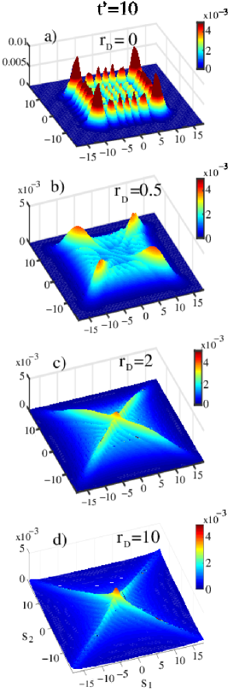
Figure 4: (Color online) Probability profile $P_{s_{1},s_{2}}(t^{\prime})$ with $t^{\prime}=t_{\Omega}=10$, for an IC $\rho(t=0)=\arrowvert\vec{0}\rangle\langle\vec{0}\arrowvert$ as a function of position of particles $s_{1}$ and $s_{2}$, for (a) $r_{D}=0$, (b) $r_{D}=0.5$. The interference pattern can be seen even in the presence of large dissipation: (c) for $r_{D}=2$ and (d) $r_{D}=10$. Blue indicates, roughly, the value zero while red the high value of probability.

Fig.4(a) corresponds to the case when the two free particles do not interact with the bath ($D\equiv\Gamma^{2}k_{B}T/\hbar=0$), here the evolution of particles are ballistic (not diffusive) and characterized by Anderson’ velocity: $V_{A}=\frac{1}{\sqrt{2}}\frac{\Omega}{\hslash}$ [24], this is a pure quantum regime. When the temperature of the bath $\mathcal{B}$ is different from zero the profile $P_{s_{1},s_{2}}(t^{\prime})$ is modified, appearing interference patterns along of line $s_{1}=s_{2}$, and raising the value of the probability in the direction $s_{1}=-s_{2}$ (conservation of total momentum), see Figs.4(b),(c). In the case $r_{D}\gg 1$ (strong dissipation case) the profile $P_{s_{1},s_{2}}(t^{\prime})$ shows a different interference pattern signing the quantum nature of the behavior, see Fig.4(d). This is in contrast to the case of two particles with independent baths, in which case the profile would be a Gaussian distribution. It is important to remark that for two DQWs with a common bath the profile can never be represented as a Gaussian distribution for any value of $r_{D}$ or $t^{\prime}$. This result says that $\mathcal{B}$ induces coherence between the particles while also producing dissipation.

4.4 Cross terms of the two-body $\rho(t)$. 

A measure to indirectly quantify the occurrence of correlations between the particles can be evaluated by calculating the total coherence contribution from the cross-terms of the density matrix. This object is defined as

$$\mathcal{G}=\sum_{\atop{}{{}{{\ (s_{1}\neq s_{1}^{\prime})\newline (s_{2}\neq s_{2}^{\prime})}}}}\left|\langle s_{1},s_{2}\arrowvert\rho(t)\arrowvert s_{1}^{\prime},s_{2}^{\prime}\rangle\right|,$$

and it has recently been used to quantify the quantum coherence [29, 30]. This measure is easy to compute than the relative coherence entropy which need a diagonalization procedure [31]In figure 5, we show the Quantum Coherence (QC) $\mathcal{G}$ as a function of $t^{\prime}=\frac{\Omega t}{\hbar}$ and for several values of dissipation $r_{D}=0,$ $0.1,$ $0.5,$ $2$. As we will see with other measures for $0<t^{\prime}<0.6\simeq\tau_{c}$ the QC is larger for the case $T\neq 0$ ($r_{D}\neq 0$) than with respect to the case $T=0$ ($r_{D}=0$). This result also indirectly indicates that thermal bath has created correlations between particles for $t^{\prime}<\tau_{c}$, and for times $t^{\prime}>\tau_{c}$ will vanish for the presence of the bath dissipation. In order to clarify the behavior of QC for $t^{\prime}>\tau_{c}$ (larger for $T=0$ than $T\neq 0$), the two extreme cases are shown in figure 6; that is, the function $\mathcal{G}$ as function of $t_{\Omega}$ for the zero dissipation case ($D=0$), and $\mathcal{G}$ as function of $t_{D}$ for the strong dissipation case ($\Omega=0$).

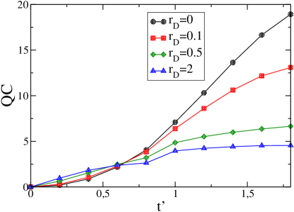
Figure 5: (Color online) Quantum coherence (QC) for two particles with IC (10) as function of $t^{\prime}=t_{\Omega}\equiv\Omega t/\hbar$. This function shows a crossover at $t^{\prime}\simeq 0.6$ as a function of time. The plot shows $\mathcal{G}$ calculated for different values of the dissipation parameter $r_{D}=\frac{2D}{\Omega/\hbar}.$

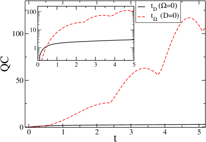
Figure 6: (Color online) Quantum coherence (QC) for two particles with IC (10) for extrema cases: zero dissipation ($D=0$), and strong dissipation ($\Omega=0$) as a function of $t^{\prime}=$ $t_{\Omega}\equiv\Omega t/\hbar$. This function shows a notable structured behavior as a function of time for the non-dissipative case. While in the strong dissipative case the behavior is monotonous increasing, showing only a suddenly increase at short times. In the inset, the function $\mathcal{G}$ is shown in logarithmic scale.

As can be seen from the exact result (19), the solution of $\rho\left(t\right)$ is a convolution of quantum and classical contributions. The signature of the quantum character appears through J-Bessel’s functions which oscillates in time ($t_{\Omega}\equiv\frac{\Omega t}{\hbar}$), while the classical functionality comes from I-Bessel’s functions (note that here the time appears through the quantity: $t_{D}\equiv 2Dt$). Therefore, it is simple to realize that the nature of the oscillations in the case $D=0$ (see figure 6) comes from the temporal behaviors of the J-Bessel’s functions. On the contrary, in the case $\Omega=0$ the function $\mathcal{G}$ is a smooth function of time (only depends on the I-Bessel’s functions).

It is important to remark that the crossing-time that we have found analyzing the QC is of the order of the scaling-time that we got from the study of the purity (see figure 3).

Numerically, the long time behavior of the function $\mathcal{G}$ is very hard to get (the solution $\rho\left(t\right)$ involves the product of four J-Bessel’s and six I-Bessel’s functions in the lattice). Nevertheless, it is not difficult to realize from (19), that if $D\neq 0$ at long time all elements of $\rho\left(t\right)$ go to zero (conserving normalization see (3)).

5 On the Wigner phase-space representation.

A novel point of view can be achieved if we introduce a quasi probability distribution function (pdf) on the lattice [32]. A similar representation was used for the case of one-particle $\rho(t)$ in reference [24]. The crucial point in the definition of a quasi-pdf is to assure the completeness of the representation, a fact that can be proved from our Wigner-like pdf.

Consider the quasi-pdf on the enlarged lattice of integers ($\mathcal{Z}$) and semi-integers ($\mathcal{Z}_{2}$), and use the notation:

$$\vec{k}=(k_{1},k_{2}),\vec{x}=(x_{1},x_{2}),x_{j}\in(\mathcal{Z}\oplus\mathcal{Z}_{2}).$$

We define

$$W\!(\vec{k},\vec{x},t)\! = \!(2\pi)^{-2}\!\!\!\!\!\!\!\!\sum_{x_{1}^{\prime},x_{2}^{\prime}\in(\mathcal{Z}\oplus\mathcal{Z}_{2})}\!\!\!\!\!\!\!\!\!\langle x_{1}\!+\!x_{1}^{\prime},x_{2}\!+\!x_{2}^{\prime}\arrowvert\rho(t)\arrowvert x_{1}\!-\!x_{1}^{\prime},x_{2}\!-\!x_{2}^{\prime}\rangle$$ (41)

$$\times \exp\left(-i2\vec{k}\cdot\vec{x}^{\prime}\right).$$

We note that Wigner function, (41), is defined over the enlarged set $(\mathcal{Z}\oplus\mathcal{Z}_{2})$ with the natural prescription

$$\langle\vec{x}\arrowvert\rho(t)\arrowvert\vec{x}^{\prime}\rangle=0,$$

which is true if some index $x_{j}\in\mathcal{Z}_{2}$ because the Wannier basis is on the field of $\mathcal{Z}$.

Our definition of Wigner function satisfies the fundamental marginal conditions [33]:

$$\int\int\limits_{-\pi}^{\pi}d\vec{k}\ W(\vec{k},\vec{x},t) = \langle\vec{x}\arrowvert\rho(t)\arrowvert\vec{x}\rangle\geq 0$$

$$\sum_{\vec{x}\in(\mathcal{Z}\oplus\mathcal{Z}_{2})}W(\vec{k},\vec{x},t) = \langle\vec{k}\arrowvert\rho(t)\arrowvert\vec{k}\rangle\geq 0$$

$$\sum_{\vec{x}\in(\mathcal{Z}\oplus\mathcal{Z}_{2})}\int\int\limits_{-\pi}^{\pi}d\vec{k}\ W(\vec{k},\vec{x},t) = 1.$$

In addition, from the discrete Fourier transform we can obtain the inverse relation on the field of integers ($\mathcal{Z}$):

$$\langle s_{1},s_{2}\arrowvert\rho(t)\arrowvert s_{1}^{\prime},s_{2}^{\prime}\rangle\! = \!\int\int\limits_{-\pi}^{\pi}d\vec{k}\ W(k_{1},k_{2},\frac{s_{1}+s_{1}^{\prime}}{2},\frac{s_{2}+s_{2}^{\prime}}{2},t)$$

$$\times \exp[i\vec{k}\cdot(\vec{s}-\vec{s}^{\prime})].$$

Note that this inverse relation demands the necessity of a quasi-pdf on the enlarged field of $(\mathcal{Z}\oplus\mathcal{Z}_{2})$. Carrying on the calculation, from Eq.(41) we arrive to

$$W(\vec{k},\vec{x},t)\! = \!\frac{e^{-2t_{D}}}{4\pi^{2}}\!\!\!\!\!\!\sum\limits_{\{\alpha,\beta,q,n_{2},n_{3},n_{5}\}\in\emph{Z}}\!\!\!\!\!\!\!\!(-1)^{2x_{1}+2x_{2}}$$ (42)

$$\times \!J_{2x_{1}+2\alpha-q}(\!-2t_{\Omega}\sin k_{1}\!)J_{2x_{2}+2\beta+q}(\!-2t_{\Omega}\sin k_{2}\!)$$

$$\times \!(-1)^{q}(-1)^{n_{2}+n_{3}}I_{n_{2}}(t_{D})I_{n_{3}}(t_{D})I_{n_{5}}(t_{D})$$

$$\times \!I_{n_{2}+n_{5}-\alpha}(t_{D})I_{n_{3}+n_{5}+\beta}(t_{D})I_{n_{2}+n_{3}+n_{5}-q}(t_{D})$$

$$\times \!\exp[iq(k_{1}-k_{2})],$$

here we have used the IC (10). The present definition is equivalent to the one proposed from phase-point operators in the reference [34]. In the case $D=0$ we obtain the well known non-dissipative description for a tight-binding

$$W(\vec{k},\vec{x},t)_{D=0}=\frac{1}{4\pi^{2}}J_{2x_{1}}(2t_{\Omega}\sin k_{1})\ J_{2x_{2}}(2t_{\Omega}\sin k_{2}),$$

this solution represents two-independent particles evolving with a unitary transformation [24].

Equation (42) can be used to detect whether a state in phase-space has a pure quantum character. This goal can be achieved by looking if $W(\vec{k},\vec{x};t)$ is negative or not. Therefore, the total negative volume in phase-space can be measured by the (positive) function:

$$\mathcal{V}(t)\!=\!\!\!\!\sum_{\vec{x}\in(\mathcal{Z}\oplus\mathcal{Z}_{2})}\int\int\limits_{-\pi}^{\pi}d\vec{k}\ \left[\left|W(\vec{k},\vec{x},t)\right|-W(\vec{k},\vec{x},t)\right]$$ (43)

We note that in a situation where the classical regime dominates this function vanishes, on the contrary in a quantum regime this function is larger than zero. Then, this measure could be used to show the quantum to classical transition. We can compare this result with the characteristic time-scale –for the maximum of coherence– that we have found using different measures in section IV.

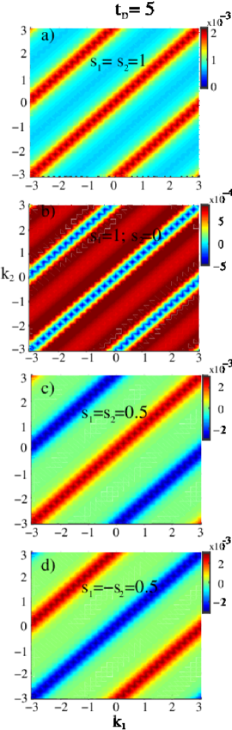
Figure 7: (Color online) Wigner quasi pdf for two particles with IC as in (10) in the Fourier plane $\{k_{1},k_{2}\}$, for time $t_{D}=2Dt=5$. The negative domains are shown in dark blue. (a), (b) Wigner function for the case: $\{s_{1}=-s_{2}=1$, $s_{1}=s_{2}=1\}$ (integers) and (c), (d) $\{s_{1}=s_{2}=0.5$, $s_{1}=-s_{2}=0.5\}$ (semi-integers).

In figure 7 we show several portraits of this pseudo pdf, in fact, it is clear to identify the domain where the Wigner function is negative. In particular, we plot $W(\vec{k},\vec{x},t)$ in the $k_{1},k_{2}$ plane for the cases $s_{1}=s_{2}$ and $s_{1}=-s_{2}$. The plots show a strip structure in the Brillouin zone and also the symmetry of the Wigner function (mirror reflection on the plane $k_{1}=k_{2}$). The blue regions (color online) correspond to negative values of the Wigner function. In general, we can propose to use $W(\vec{k},\vec{x},t)$ to point out the quantum to classical transition as a function of the dissipative parameter $r_{D}\equiv\frac{2D}{\Omega/\hbar}$ and the dimensionless time $t^{\prime}=t_{\Omega}$.

In figure 8 we show the absolute value of the negative volume $\mathcal{V}(t)$ as a function of $t^{\prime}=\frac{\Omega t}{\hbar}$, and for different values of $r_{D}$. From this plot we reach to the conclusion that for times $0<t^{\prime}<\tau_{c}^{\prime}$ the negative volume is larger for the case $T\neq 0$ than with respect to the case $T=0$, indirectly indicating the quantum character of the correlations. This behavior is similar to the one that we got analyzing the QC (see Section 4.D). We want remark that $\tau_{c}^{\prime}$ is similar to the scaling-time obtained from QC (see Fig. 5), and $\tau_{M}$ from the GQD see Fig. 10.

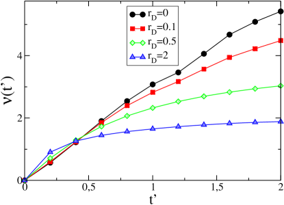
Figure 8: (Color online) Absolute value of the negative volume of the Wigner function for two particles as a function of $t^{\prime}=\frac{\Omega t}{\hbar}$. Here we have used the same parameters as in figure 5, then the quantum character of the correlations is indicated by the non-zero value of this volume $\mathcal{V}(t)$.

From Eq.(42) we can also see that if $\Omega=0$ the expression simplify notably:

$$W(\vec{k},\vec{x},t)_{\Omega=0} = \frac{e^{-2t_{D}}}{4\pi^{2}}\sum\limits_{\{q_{1},q_{2}\}\in\emph{Z}}(-1)^{q_{1}+q_{2}}J_{q_{1}+x_{1}}(2Dt)$$

$$\times \!J_{q_{2}-x_{2}}(2Dt)I_{q_{2}+q_{1}}(2Dt\cos\left(k_{2}-k_{1}\right))$$

$$\times \!I_{q_{1}-q_{2}}(2Dt\cos\left(k_{2}\!-\!k_{1}\right))I_{n_{2}+n_{3}+n_{5}-q}(t_{D})$$

$$\times \!\exp[iq(k_{1}-k_{2})].$$

Then, it is possible to check that Wigner function has an interference pattern even in the high dissipative regime $r_{D}\gg 1$, see figure 7. It is easy to see that in the case $\Omega=0$ it is also possible to find phase-space domains where this quasi-pdf is negative.

6 Quantum Correlations

Different methods for characterizing the quantum and classical parts of correlations is an active topics in quantum information theory [13]. An important part of the quantum information community consider the Quantum Discord (QD) as a suitable measure of quantum correlations [11]. Nevertheless there are some criticisms on this measure because QD is not contractive under general local operations and therefore should not be regarded as a strict measure for that purpose. Despite this issue, and in order to compute an analytical expression for characterizing correlations in our system, we have to argue in favor of QD [12]. Related with the QD is the geometric quantum discord (GQD) [35]. In particular, we use here, for such purpose, the GQD which is easier to calculate than the QD (this measure involves an optimization procedure), and it has been proved to be a necessary and sufficient condition for non-zero QD [35].

6.1 Geometric quantum discord of bipartite states. 

The geometric measure of quantum discord (GQD) has been defined as

$$D_{G}\left(\rho\right)=\min_{\chi\in\Omega_{0}}\left|\left|\rho-\chi\right|\right|^{2},$$ (44)

where $\Omega_{0}$ denotes the set of zero-discord states and $\left|\left|X-Y\right|\right|^{2}=\mbox{Tr}\left(X-Y\right)^{2}$ is the square norm in the Hilbert-Schmidt space. The lower bound of the GQD can be calculated using that the density operator on a bipartite system belonging to $H^{a}\otimes H^{b}$, with $\dim H^{a}=m$ and $\dim H^{b}=n$, can be written in the form [35, 36, 37, 38]:

$$\rho = \frac{1}{mn}\left(\mathbf{I}_{m}\otimes\mathbf{I}_{n}+\sum_{i}x_{i}\tilde{\lambda}_{i}\otimes\mathbf{I}_{n}+\sum_{j}y_{j}\mathbf{I}_{m}\otimes\tilde{\lambda}_{j}\right.$$

$$+\left.\sum_{j}t_{ij}\tilde{\lambda}_{i}\otimes\tilde{\lambda}_{j}\right),$$

where $\tilde{\lambda}_{i},i=1,\cdots,m^{2}-1$ and $\tilde{\lambda}_{j},j=1,\cdots,n^{2}-1$ are the generators of $SU(m)$ and $SU(n)$ respectively, satisfying $\mbox{Tr}\left(\tilde{\lambda}_{i}\tilde{\lambda}_{j}\right)=2\delta_{ij}$. In this expression the vectors $\vec{x}\in\emph{R}^{m^{2}-1}$ and $\vec{y}\in\emph{R}^{n^{2}-1}$ of the subsystems $A$ and $B$ are given by:

$$x_{i} = \frac{m}{2}\mbox{Tr}\left(\rho\tilde{\lambda}_{i}\otimes\mathbf{I}_{n}\right)=\frac{m}{2}\mbox{Tr}\left(\rho_{A}\tilde{\lambda}_{i}\right)$$

$$y_{j} = \frac{m}{2}\mbox{Tr}\left(\rho\mathbf{I}_{m}\otimes\tilde{\lambda}_{j}\right)=\frac{n}{2}\mbox{Tr}\left(\rho_{B}\tilde{\lambda}_{j}\right),$$

and the correlation matrix $T\equiv\left[t_{ij}\right]$ is given by

$$T\equiv\left[t_{ij}\right]=\frac{mn}{4}\mbox{Tr}\left(\rho\tilde{\lambda}_{i}\otimes\tilde{\lambda}_{j}\right).$$

The lower bound of the GQD can be written as:

$$D_{G}\left(\rho\right)\geq\frac{2}{m^{2}n}\left(\left|\left|\vec{x}\right|\right|^{2}+\frac{2}{n}\left|\left|T\right|\right|^{2}-\sum_{i=1}^{m-1}\eta_{i}\right),$$ (46)

where $\eta_{i},i=1,2,\cdots,m^{2}-1$ are eigenvectors of the matrix $\left(\vec{x}\vec{x}^{t}+\frac{2}{n}TT^{t}\right)$ arranged in non-increasing order [36].

For our present model ($2$ particles in an infinite lattice), we need to introduce a bipartition on the lattice to study the GQD (a similar bipartition was used for a $1$-particle Hamiltonian system in Ref. [15]), therefore introducing a bipartition we will end with a qutrit-qutrit system. In our case $m=n=3$ and we can use the $SU(3)$ representation for calculating the GQD [37] in terms of the Gell-Mann matrices $\tilde{\lambda}_{j}$.

6.2 The mirror bipartition for a $2$ particles system

In our case $\rho\left(t\right)$ has a diffusion-like time-behavior limited by the quantum unitary evolution (see Eq. 19). Then, our calculation would consist in assuming that for a fixed time “$t$” the DQW has evolved in a finite domain supported by the basis of generators $SU(M_{t}),$ with $M_{t}\gg 1$ (see 6.1). Our approximation consists in calculating the GQD under the $SU(3)$ projection neglecting all no-mirror effects in the infinite lattice using (46). A similar procedure was used for a spin system under the $SU\left(2\right)$ projection [39]

In figure 9 we show the mirror bipartition that we are going to use for the present $2$-body system, i.e., we trace out sites on the rest of the lattice, keeping only two sites $\pm s$ in order to define a three-level system; this bipartition allows us to calculate the GQD $D_{G}^{\left(s\right)}\left(\rho_{AB}\right).$ In other words, the density matrix $\rho_{AB}$ corresponds to the subset $AB$, that is: particles $1$ or $2$ can be at sites $\pm s$ or in the complement subset $R$ (the rest of the lattice). Then it is clear that using this bipartition we have built up a couple qutrit-qutrit using the sites $\pm s$ on the lattice.

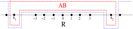
Figure 9: Graphical representation of the bipartition on the lattice, the sites $s_{1}=-s$ and $s_{2}=s$ are part of the subset $AB$, and the remaining sites in the lattice is the complement subset $R$. The set $AB$ represents a qutrit-qutrit system. Then particles $1$ and $2$ can be either in the set $AB$ or in $R$.

In order to trace out sites $s^{\prime}\neq\pm s$ note that for one particle we can associate the kets

$$\arrowvert A\rangle \leftrightarrow \arrowvert s\rangle$$

$$\arrowvert B\rangle \leftrightarrow \arrowvert-s\rangle$$

$$\arrowvert\phi\rangle \leftrightarrow \arrowvert s^{\prime}\rangle,\ s^{\prime}\neq\pm s.$$

For $2$-particles the ket $\arrowvert s_{1},s_{2}\rangle$ can be written in the form

$$\arrowvert s_{1},s_{2}\rangle=\arrowvert\alpha\beta\rangle\otimes\arrowvert R\rangle,$$ (47)

where $\left\{\alpha,\beta\right\}\in\left\{A,B,\phi\right\}$, and $R\$is the complement, i.e., the set of sites, which are different from $\pm s$.

Using (47) in our expression for the $2$-body density matrix (19) we can calculate analytically the density matrix $\rho_{AB}$ for the bipartition of figure 9. This matrix turns to be a reduced $\left(9\times 9\right)$ density matrix, i.e., it can be written in the ordered basis:

$$\{\arrowvert AA\rangle,\arrowvert AB\rangle,\arrowvert A\phi\rangle,\arrowvert BA\rangle,\arrowvert BB\rangle,\arrowvert B\phi\rangle,\arrowvert\phi A\rangle,\arrowvert\phi B\rangle,\arrowvert\phi\phi\rangle\}$$

In order to calculate the lower bound of the GQD we use the total mirror contribution for the GQD, which is defined as

$$D_{G}^{T}\left(\rho_{AB}\right)=\frac{d}{d-1}\sum_{s=1}^{\infty}D_{G}^{\left(s\right)}\left(\rho_{AB}\right),$$ (48)

where $D_{G}^{\left(s\right)}\left(\rho_{AB}\right)$ corresponds to (46) for a fixed value of $s$, here $d/(d-1)$ (which in our case turns to be $3/2$) is a normalization factor. In fact the GQD can also be defined through alternatives norms [40], here we used the norm$-2$ from references [41], which by the way is equivalent to the expression in [38].

Then the value $D_{G}^{\left(s\right)}\left(\rho_{AB}\right)$ measures the quantum correlation between particles $1$ and $2$ to be confined at sites $\pm s.$ Using the dimensionless parameter $r_{D}=2D/(\Omega/\hbar)$ and the time $t^{\prime}=(\Omega/\hbar)t$ we have plotted $D_{G}^{T}\left(\rho_{AB}\right)$ as a function of time, for different values of the temperature of the bath ($D\equiv\Gamma^{2}k_{B}T/\hbar$). In figure 10 we show the GQD (lower bound given by 46) for three values of $r_{D}$, from this plot it is possible to see that the correlations induced between the particles are in fact of quantum nature because $D_{G}^{T}\left(\rho_{AB}\right)>0$ for almost all $t>0$ (for the case $r_{D}=0.5$ and at short times –apart form numerical errors– it seems to be negative). Then, several important conclusions can be drawn.

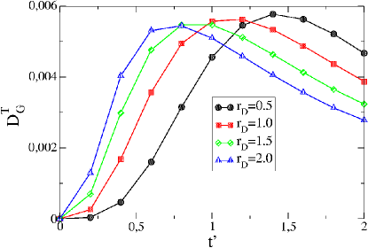
Figure 10: Geometrical quantum discord calculated from the bipartition of figure 9. The function $D_{G}^{T}\left(\rho_{AB}\right)$ takes into account all the mirror contributions as defined in (48). This function is associated to a qutrit-qutrit system and represents the quantum correlations (bath-generated) between the two particles. As noted there is a characteristic time $\tau_{M}$ when these correlations are maxima.

First: The bath-induced quantum correlation is time dependent showing a non-monotonic behavior, with a maximum at a characteristic time-scale $\tau_{M}$ that depends on the dissipative parameter $r_{D}$. After this time quantum correlations are wiped out by the dissipation.

Second: If the temperature of the bath decreases the characteristic time $\tau_{M}$ is delayed. If $r_{D}=0$ the GQD vanishes at all times.

Third: The bath-induced quantum correlation would vanish monotonically at long-time as a result of the dissipation (we could not run the long-time behavior because we have numerical errors). The behavior of $D_{G}^{T}\left(\rho_{AB}\right)$ as a function of time $t^{\prime}$ has a response (with a maximum) with a similar time-scale as the one from the QC and the negative volume of the Wigner function.

7 Conclusions.

We have analyzed two free spinless particles –in a 1D regular lattice– interacting with a common thermal phonon bath $\mathcal{B}$. We have solved analytically the associated QME for the two (initially uncorrelated) distinguishable particles to characterize the quantumness of the correlations induced by $\mathcal{B}$.

Some measures like spatiotemporal correlation function $\mathcal{C}_{(1,2)}$, quantum coherence $\mathcal{G}$, purity, entropy, quantum mutual information have been analyzed showing a high degree of coherence between the two particles. Then, pointing out that this result is in fact induced by the common bath, despite the existing dissipation for temperatures different from zero ($D\equiv\Gamma^{2}k_{B}T/\hbar$ where $T$ is the temperature of $\mathcal{B}$). The purity, quantum mutual information, and the quantum coherence $\mathcal{G}$ has been used to find a characteristic time-scale to show when the coherence has a maximum value. We have find a similar time-scale value for all these measures.

All these results have also been supported by the analysis of a Wigner-like function which shows domains (in a lattice phase-space) being negative. We have calculated the (absolute value) of the negative volume $\mathcal{V}(t)$ of the Wigner pdf as a function of time $t^{\prime}=\frac{\Omega t}{\hbar}$ and for several values of dissipative parameter $r_{D}$. In fact the negative volume also shows a characteristic time-scale in its behavior which is in agreement with our calculations made with other quantum measures of coherence as the purity, off-diagonal quantum coherence, and quantum mutual information. Thus the negative volume may be considered as an indirect indicator of quantum properties.

As a criterion to check the quantum nature of the process we have also calculate the GQD. To do this we introduce a bipartition in the lattice in order to associate a qutrit-qutrit set from our $2$-particle system, thus we showed that $D_{G}^{T}\left(\rho_{AB}\right)>0$ for some values of $r_{D}$ and $t^{\prime}>0$, which would indicate the quantum nature of the induced correlations between the particles. In fact the time behavior of the $D_{G}^{T}\left(\rho_{AB}\right)$ is an increasing function of time showing a maximum at a characteristic time $\tau_{M}$, which is of the order of the time-scale that we have found analyzing the QC and the Wigner function. After this time $\tau_{M}$ the behavior of the GQD is decreasing approaching zero.

The profile of probability for two particles is ballistic for $D=0$ (the closed system corresponds to the tight-binding model) and it starts to be modified by the presence of temperature ($D>0$), showing a notable X-form pattern in the presence of dissipation. In the case of larger values of the dissipation parameter $r_{D}\equiv\frac{2D}{\Omega/\hbar}\gg 1$ this structure is accentuated and additional interference patterns are also observed as a result of the interaction with the thermal bath $\mathcal{B}$.

Our approach opens the possibility of performing analytical analysis on important quantities related to quantum correlation measures in dissipative bipartite systems [14, 15], for example the quantum discord for a qutrit-qutrit set as we have shown in this work. In addition from the present approach it is possible to write down an equivalent QME for more than two (free) bosonic or fermionic particles interacting with a common bath, these results are of great interest in nanoscience and quantum information theory, and will be presented in future contributions. Then, our analysis could be of interest in experiments using –for example– photonic devices similar to the ones of Refs. [42, 43].

Acknowledgments. M.O.C gratefully acknowledges support received from CONICET, grant PIP 112-201501-00216 CO, Argentina.

Appendix A: Fock representation for Bosonic particles

In this appendix, we prove the equivalence between the Fock representation and the Wannier basis. In particular we will work out bosonic particles in Fock’s space and symmetric Wannier’s states. A similar equivalent demonstration can be done for fermionic particles. Let us define the creation operators $C_{s_{1}}^{\dagger},C_{s_{2}}^{\dagger}$ acting on the vacuum state $\arrowvert\phi\rangle$. Fock’s basis can be denoted as

$$C_{s_{1}}^{\dagger}C_{s_{2}}^{\dagger}\arrowvert\phi\rangle\!=\!\arrowvert\cdots,0,\cdots,1,0,\cdots,1,0,\cdots,\cdots,0,\cdots\rangle,$$ (49)

i.e., it has been created two indistinguishable particles at sites $s_{1}$ and $s_{2}$. If these particles are bosonic the operators $C_{s_{1}}^{\dagger},C_{s_{2}}^{\dagger}$ and $C_{s_{1}},C_{s_{2}}$ satisfy the relations

$$\left[C_{s_{1}},C_{s_{2}}^{\dagger}\right]=\delta_{s_{1},s_{2}};\ \left[C_{s_{1}},C_{s_{2}}\right]=\left[C_{s_{1}}^{\dagger},C_{s_{2}}^{\dagger}\right]=0.$$ (50)

Let the translation operator be defined as

$$R=\sum_{s=-\infty}^{\infty}C_{s-1}^{\dagger}C_{s}$$ (51)

Therefore, using (50) we can prove that $R$ translates (individually) two indistinguishable particles

$$RC_{s_{1}}^{\dagger}C_{s_{2}}^{\dagger}\arrowvert\phi\rangle = \sum_{s=-\infty}^{\infty}C_{s-1}^{\dagger}C_{s}C_{s_{1}}^{\dagger}C_{s_{2}}^{\dagger}\arrowvert\phi\rangle$$ (52)

$$= \sum_{s=-\infty}^{\infty}C_{s-1}^{\dagger}\left(\delta_{s,s_{1}}+C_{s_{1}}^{\dagger}C_{s}\right)C_{s_{2}}^{\dagger}\arrowvert\phi\rangle$$

$$= C_{s_{1}-1}^{\dagger}C_{s_{2}}^{\dagger}\arrowvert\phi\rangle$$

$$+ \sum_{s=-\infty}^{\infty}C_{s-1}^{\dagger}C_{s_{1}}^{\dagger}\left(\delta_{s,s_{2}}+C_{s_{2}}^{\dagger}C_{s}\right)\arrowvert\phi\rangle$$

$$= C_{s_{1}-1}^{\dagger}C_{s_{2}}^{\dagger}\arrowvert\phi\rangle+C_{s_{2}-1}^{\dagger}C_{s_{1}}^{\dagger}\arrowvert\phi\rangle,$$

here we have used that $C_{s}\arrowvert\phi\rangle=0.$ In a similar way, noting that

$$R^{\dagger}\!\!=\!\!\sum_{s=-\infty}^{\infty}\left(C_{s-1}^{\dagger}C_{s}\right)^{\dagger}\!\!=\!\!\!\!\sum_{s=-\infty}^{\infty}C_{s}^{\dagger}C_{s-1}=\sum_{s^{\prime}=-\infty}^{\infty}C_{s^{\prime}+1}^{\dagger}C_{s^{\prime}},$$ (53)

it is simple to prove that

$$R^{\dagger}C_{s_{1}}^{\dagger}C_{s_{2}}^{\dagger}\arrowvert\phi\rangle=C_{s_{1}+1}^{\dagger}C_{s_{2}}^{\dagger}\arrowvert\phi\rangle+C_{s_{2}+1}^{\dagger}C_{s_{2}}^{\dagger}\arrowvert\phi\rangle.$$ (54)

For the calculation of the infinitesimal Kossakoswki-Lindbland generator it is important to know the action of the operator $R^{\dagger}R$. To calculate this operator, we use the definition of $R^{\dagger},R$ and (50), then we get

$$RR^{\dagger} = \sum_{s=-\infty}^{\infty}C_{s-1}^{\dagger}C_{s}\sum_{s^{\prime}=-\infty}^{\infty}C_{s^{\prime}+1}^{\dagger}C_{s^{\prime}}$$

$$= \sum_{s^{\prime}=-\infty}^{\infty}C_{s^{\prime}}^{\dagger}C_{s^{\prime}}+\sum_{s=-\infty}^{\infty}\sum_{s^{\prime}=-\infty}^{\infty}C_{s-1}^{\dagger}C_{s^{\prime}+1}^{\dagger}C_{s}C_{s^{\prime}}.$$

Therefore

$$RR^{\dagger}C_{s_{1}}^{\dagger}C_{s_{2}}^{\dagger}\arrowvert\phi\rangle = 2C_{s_{1}}^{\dagger}C_{s_{2}}^{\dagger}\arrowvert\phi\rangle+C_{s_{1}-1}^{\dagger}C_{s_{2}+1}^{\dagger}\arrowvert\phi\rangle$$ (55)

$$+ C_{s_{1}+1}^{\dagger}C_{s_{2}-1}^{\dagger}\arrowvert\phi\rangle.$$

In a similar way we can also prove that $RR^{\dagger}=R^{\dagger}R$, therefore, for boson particles $R$ and $R^{\dagger}$ commute, i.e., $\left[R,R^{\dagger}\right]=0.$

Now we are going to show that the same algebra can be obtained using a symmetrized Wannier’s basis. This is an important result for calculating the infinitesimal generator. Let the symmetric Wannier vector state (for two particles) be written in the form

$$\arrowvert s_{1},s_{2}\rangle_{S}=\frac{1}{\sqrt{2}}\left[\arrowvert s_{1},s_{2}\rangle+\arrowvert s_{2},s_{1}\rangle\right].$$

In order to compare both algebras –in Fock and Wannier spaces– we need to know the action of translation operators in the symmetric Wannier representation. Then, from (54) we can define the action of the translation operator $T_{12}$ for indistinguishable particles as

$$T_{12}\arrowvert s_{1},s_{2}\rangle_{S}=\arrowvert s_{1}-1,s_{2}\rangle_{S}+\arrowvert s_{1},s_{2}-1\rangle_{S}$$ (56)

$$T_{12}^{\dagger}\arrowvert s_{1},s_{2}\rangle_{S}=\arrowvert s_{1}+1,s_{2}\rangle_{S}+\arrowvert s_{1},s_{2}+1\rangle_{S}.$$ (57)

These operators produce the same state as when $R$ and $R^{\dagger}$ are applied to Fock’s vector state. To end this appendix we can calculate here the action of $T_{12}^{\dagger}T_{12}$ on a symmetric Wannier’s state, from (56) and (57) we get

$$T_{12}^{\dagger}T_{12}\arrowvert s_{1},\!s_{2}\rangle_{S}\!=\!2\arrowvert s_{1},\!s_{2}\rangle_{S}+\arrowvert s_{1}-1,\!s_{2}+1\rangle_{S}+\arrowvert s_{1}+1,\!s_{2}-1\rangle_{S}$$

with $\left[T_{12}^{\dagger},T_{12}\right]=0$. Therefore, the action of $T_{12}^{\dagger}T_{12}$ on a symmetric Wannier state is equivalent to the action of $R^{\dagger}R$ on a Bosonic Fock state (55). Similar calculation can be done for fermionic particles.

Appendix B: The two-body reduced density matrix from a pure interacting infinitesimal generator

Consider the infinitesimal generator for two distinguishable DQW in the Fourier representation (14). If we want to solve a pseudo-density matrix $\Pi(t)$ taking into account only the bath-mediated interacting term; then, the evolution equation will be

$$\frac{d}{dt}\!\left\langle k_{1},\!k_{2}\left|\Pi(t)\right|k_{1}^{\prime},\!k_{2}^{\prime}\right\rangle\!\!=\!\!\mathcal{I}\!\left(k_{1},k_{2},\!k_{1}^{\prime},\!k_{2}^{\prime}\right)\!\left\langle k_{1},k_{2}\left|\Pi(t)\right|k_{1}^{\prime},\!k_{2}^{\prime}\right\rangle\!,$$ (58)

with

$$\mathcal{I}\left(k_{1},k_{2},k_{1}^{\prime},k_{2}^{\prime}\right)\!\! = \!\!2D[\mathbf{C}\left(k_{1}\!,k_{2}^{\prime}\right)\!+\!\mathbf{C}\left(k_{2}\!,k_{1}^{\prime}\right)\!-\!\mathbf{C}\left(k_{1}\!,k_{2}\right)$$ (59)

$$- \!\!\mathbf{C}\left(k_{1}^{\prime}\!,k_{2}^{\prime}\right)].$$

If the IC is $\Pi(0)=\arrowvert s_{1}^{0},s_{2}^{0}\rangle\langle s_{1}^{0},s_{2}^{0}\arrowvert$, the solution will be given by the Fourier antitransform

$$\left\langle s_{1},s_{2}\left|\Pi(t)\right|s_{1}^{\prime},s_{2}^{\prime}\right\rangle\! = \!\left(2\pi\right)^{-4}\int\int\int\int dk_{1}\!\!\ dk_{1}^{\prime}\!\!\ dk_{2}\!\!\ dk_{2}^{\prime}$$

$$\times \!e^{ik_{1}(s_{1}-s_{1}^{0})}e^{ik_{1}^{\prime}(-s_{1}^{\prime}+s_{1}^{0})}$$

$$\times \!e^{ik_{2}(s_{2}-s_{2}^{0})}e^{ik_{2}^{\prime}(-s_{2}^{\prime}+s_{2}^{0})}e^{\mathcal{I}\left(k_{1},k_{2},k_{1}^{\prime}k_{2}^{\prime}\right)t}\!,$$

using $e^{x\cos\theta}=\sum_{n=-\infty}^{\infty}I_{n}(x)e^{in\theta}$, and after some algebra (noting that $I_{n}(-x)=(-1)^{n}I_{n}(x)$ and using (21)-(22)) we get

$$\left\langle s_{1},s_{2}\left|\Pi(t)\right|s_{1}^{\prime},s_{2}^{\prime}\right\rangle\! = \!\delta_{s_{1},s_{2},s_{1}^{\prime},s_{2}^{\prime}}\sum_{n_{4}\in\mathcal{Z}}I_{-s_{2}^{\prime}+s_{2}^{0}-n_{4}}(t_{D})$$ (60)

$$\times \!I_{-s_{1}^{\prime}+s_{1}^{0}-n_{4}}(t_{D})I_{s_{2}-s_{2}^{0}-s_{1}^{\prime}+s_{1}^{0}+n_{4}}(t_{D})$$

$$\times \!I_{n_{4}}(t_{D}),$$

from this result it is simple to see that this solution is normalized $\mbox{Tr}\left[\Pi(t)\right]=1.$ Two interesting conclusions can also be drawn from (60): the first is concerning the Purity of the two-body system, and the second is about the one-body reduced density matrix.

1) From the solution (60), and after some algebra, we can calculate the Purity associated to the pseudo density matrix

$$\mathcal{P}_{Q}(t) = \mbox{Tr}[\Pi(t)^{2}]$$

$$= \sum_{n=-\infty}^{\infty}\left(-1\right)^{n+s_{1}^{0}-s_{2}^{0}}\ I_{n+s_{1}^{0}-s_{2}^{0}}^{4}(2t_{D})$$

$$= \sum_{m=-\infty}^{\infty}\left[\left(-1\right)^{m}\ I_{m}^{2}(2t_{D})\right]^{2}\equiv\sum_{m=-\infty}^{\infty}\beta_{m}^{2}.$$

Therefore we conclude that “the eigenvalues” (for fixed time $t$) of this two-body pseudo density matrix are not necessarily positive $\beta_{m}=\left(-1\right)^{m}\ I_{m}^{2}(2t_{D})$.  This result comes from the fact that $\mathcal{I}\left(k_{1},k_{2},k_{1}^{\prime}k_{2}^{\prime}\right)$ is not a complete infinitesimal generator. The present analysis only helps to give us light into the meaning of the bath-mediated interaction term.

2) Tracing over one particle, say label $``2``$, we get

$$\langle s_{1}|\Pi^{(1)}(t)|s_{1}^{\prime}\rangle)\!=\!\langle s_{1}\arrowvert\mbox{Tr}_{2}[\Pi(t)]\arrowvert s_{1}^{\prime}\rangle\!=\!(\!-1\!)^{s_{1}+s_{1}^{0}}\delta_{s_{1},s_{1}^{0}}\delta_{s_{1},s_{1}^{\prime}},$$

then, this pseudo one-body solution does not evolve in time. This conclusion is consistent with the interpretation of the bath-mediated interaction (59) that we have used to calculate the time evolution of the pseudo density matrix $\Pi(t)$ in (58).

References

- [1] R. Alicki and K. Lendi, Quantum Dynamical Semigroups and Applications (Spronger Verlag), Lecture Notes in Physics, V.286, Berlin,(1987).
- [2] E. Joos et al, Decoherence and the Appearance of a Classical World in Quantum Theory (Springer, Berlin, 2003).
- [3] H.P. Breuer and F. Petrucione, The theory of open quantum systems, (Oxford University Press, Oxford, 2003).
- [4] N. G. van Kampen, J. Stat. Phys. 115, 1057, (2004).
- [5] A. E. Allahverdyan, R. Balian and T. M. Nieuwenhuizen, Phys. Report 525, 1-166, (2013).
- [6] A.A. Budini, A. K. Chattah, and M.O. Cáceres, J. Phys. A Math. and Gen. 32, 631 (1999).
- [7] F. Benatti et al., J. Math. Phys. 57, 062208 (2016); R. Tanas et al., J. Opt. B: Quantum Semiclass. Opt 6, S90 (2004); M. Mohseni et al., Jour. of Chem. Phys. 129, 174106 (2008); G. L. Giorgi et al., Phys. Rev. A 88, 042115 (2013).
- [8] Y. Aharonov, L. Davidovich, and N. Zagury, Phys. Rev. A 48, 1687 (1993).
- [9] N.G. van Kampen; J. Stat. Phys. 78, 299 (1995).
- [10] Oliver Mülken and Alexander Blumen, Phys. Rev. E, 71, 036128 (2005).
- [11] L. Henderson and V. Vedral, J. Phys. A 34, 6899 (2001); H. Ollivier and W.H. Zurek, Phys. Rev. Lett. 88, 017901 (2001).
- [12] K. Modi, A. Brodutch, H. Cable, T. Paterek, and V. Vedral, Rev. of Mod. Phys. 84, 1655 (2012).
- [13] M. Nielsen and I. Chuang, Quantum Computation and Quantum Information (Cambridge University Press, Cambridge, (2000).
- [14] M. Nizama and M. O. Cáceres, Physica A 392, 6155, (2013).
- [15] M. Nizama and M. O. Cáceres, Physica A 400, 31 (2014).
- [16] F. Zahringer, G. Kirchmair, R. Gerritsma, E. Solano, R. Blatt, and C. F. Roos, Phys. Rev. Lett. 104, 100503 (2010)
- [17] A. Schreiber, K. N. Cassemiro, V. Potocek, A. Gabris, I. Jex, and Ch. Silberhorn, Phys. Rev. Lett. 106, 180403 (2011).
- [18] M. A. Broome, A. Fedrizzi, B. P. Lanyon, I. Kassal, A. Aspuru-Guzik, and A. G. White, Phys. Rev. Lett. 104, 153602 (2010).
- [19] H. Schmitz, R. Matjeschk, Ch. Schneider, J. Glueckert, M. Enderlein, T. Huber, and T. Schaetz, Phys. Rev. Lett. 103, 090504 (2009).
- [20] M. Karski et al., Science 325, 174 (2009).
- [21] C. A. Ryan, M. Laforest, J. C. Boileau, and R. Laflamme, Phys. Rev. A 72, 062317 (2005).
- [22] J. Kempe, Contemp. Phys. 44, 307 (2003).
- [23] M. O. Cáceres and M. Nizama, J. Phys. A: Math. Theor. 43 455306 (2010).
- [24] M. Nizama and M. O. Cáceres, J. Phys. A: Math. Theor. 45, 335303 (2012).
- [25] E. A. Evangelidis, J. Math. Phys. 25, 2151 (1984).
- [26] L.E. Reichl, A Modern Course in Statistical Mechanics (Edward Arnold (Publishers) LTD), University of Texas Press, (1980).
- [27] M.O. Cáceres, Non-equilibrium Statistical Physics with Application to Disordered Systems, ISBN 978-3-319-51552-6, Springer (2017).
- [28] N. P. Papadakos, (arxiv.org) quant-ph/0201057 (2002).
- [29] T. Baumgratz, M. Cramer, and M. B. Plenio, Phys. Rev. Lett. 113, 140401 (2014).
- [30] Mauro B. Pozzobom and Jonas Maziero (arxiv.org) quant-ph/1605.04746 (2016).
- [31] K. Bu, Swati, U. Singh, and J. Wu, Phys. Rev. A 94, 052335 (2016).
- [32] W. K. Wootters, Phys. Rev. Lett. 80, 2245 (1998).
- [33] M. Hillery, R. F. O’Connell, M. O. Scully and E. P. Wigner, Phys. Rep. 106, 121 (1984).
- [34] M. Hinarejos, A. Pérez and M. C. Bañuls, New J. of Phys. 14, 103009, (2012).
- [35] B. Dakic, V. Vedral, and C. Brukner, Phys. Rev. Lett. 105, 190502 (2010).
- [36] A. S. M. Hassan, B. Lari, and P. S. Joag, Phys. Rev. A. 85, 0243202 (2012).
- [37] S. Rana, and P. Parashar, arXiv:1201.5969v2[quant-ph] 13 Feb 2012.
- [38] Sal Vinjanampathy and A.R.P. Rau, J. Phys. A 45, 095303 (2012).
- [39] P. Zanardi et al. J. Phys. A Math. Gen. 35, 7947 (2002).
- [40] F. M. Paula, T.R. de Oliveira, and M. S. Sarandy, Phys. Rev. A 87, 064101 (2013).
- [41] D. Girolami, and G. Adesso, arXiv:1111.3643v1[quant-ph] 15 Nov 2011.
- [42] A. Peruzzo, M. Lobino, J. C. F. Matthews, N. Matsuda, A. Politi, K. Poulios, X. Zhou, Y. Lahini, N. Ismail, K. Worhoff, Y. Bromberg, Y. Silberberg, M. G. Thompson, J. L. OBrien, Science 329, 1500 (2010).
- [43] Hagai B. Perets, Yoav Lahini, Francesca Pozzi, Marc Sorel, Roberto Morandotti, and Yaron Silberberg, Phys. Rev. Lett. 100, 170506 (2008).