$\rho$ and $K^{*}$ resonances on the lattice at nearly physical quark masses and $N_{f}=2$

Abstract

Working with a pion mass $m_{\pi}\approx 150\,\textmd{MeV}$, we study $\pi\pi$ and $K\pi$ scattering using two flavours of non-perturbatively improved Wilson fermions at a lattice spacing $a\approx 0.071\,\textmd{fm}$. Employing two lattice volumes with linear spatial extents of $N_{s}=48$ and $N_{s}=64$ points and moving frames, we extract the phase shifts for $p$-wave $\pi\pi$ and $K\pi$ scattering near the $\rho$ and $K^{*}$ resonances. Comparing our results to those of previous lattice studies, that used pion masses ranging from about $200\,\textmd{MeV}$ up to $470\,\textmd{MeV}$, we find that the coupling $g_{\rho\pi\pi}$ appears to be remarkably constant as a function of $m_{\pi}$.

I Introduction

Lattice QCD calculations are particularly suited for studies of hadrons which are stable under the strong interaction and their properties can be determined by studying correlation functions at large Euclidean time separations. However, almost all known hadrons are unstable resonances, which complicates the situation. The $\rho$ meson, one of the simplest resonances in QCD, couples to a pair of pions with total isospin $I=1$. In a finite lattice volume of linear spatial size $L=N_{s}a$, the allowed momenta of the pion pair are quantized. Neglecting $\pi\pi$ interactions, the lowest lying $\pi\pi$ state with the same spin $J=1$ as the $\rho$ has the energy

$$E_{\pi\pi}^{\mathrm{free}}=2\sqrt{m_{\pi}^{2}+\left(\frac{2\pi}{L}\right)^{2}}\,.$$ (1)

The $\rho$ can only be treated as a stable particle if its mass is sufficiently smaller than this $\pi\pi$ centre of momentum frame energy $E_{\pi\pi}^{\mathrm{free}}$. This is possible if the pion is heavy or the lattice size is small. For the values of $m_{\pi}$ and $L$ that are now accessible in lattice simulations this is not the case anymore.

The formalism for dealing with resonances in lattice QCD simulations of two-particle scattering systems has been developed first with equal masses and in systems at rest Lüscher (1991, 1986) and later extended to various moving frames and unequal masses Rummukainen and Gottlieb (1995); Kim et al. (2005); Christ et al. (2005); Feng et al. (2011); Davoudi and Savage (2011); Fu (2012); Leskovec and Prelovsek (2012); Göckeler et al. (2012). In $\pi\pi$ scattering, the $\rho$ appears as an increase of the scattering phase shift from zero to $\pi$ as the centre of momentum frame energy, $E_{cm}$, is varied from below to above the resonant mass value $m_{\rho}$. The dependence of the $\ell=1$ angular momentum partial wave shift $\delta$ on $E_{cm}$ gives detailed information about the nature of the resonance. To first approximation, the resonant mass can be extracted at the value $\delta=\pi/2$.

Due to the computational cost, previous calculations of the resonance parameters were restricted to unphysically large pion masses (most even employed pion masses with $E_{\pi\pi}^{\mathrm{free}}>m_{\rho}$), but the expected phase shift behaviour was still observed Aoki et al. (2007); Feng et al. (2011); Frison et al. (2010); Lang et al. (2011); Aoki et al. (2011); Pelissier and Alexandru (2013); Dudek et al. (2013); Fahy et al. (2015); Wilson et al. (2015a); Bulava et al. (2015); Guo and Alexandru (2015). Algorithmic advances and increases in compute power now enable us to pursue the first scattering study at a close to physical pion mass $m_{\pi}\approx 150\,\textmd{MeV}$.

The strange-light analogue of the light-light $\rho$ meson is the $K^{*}$. Its phase shift has also been studied previously in lattice calculations at unphysically large pion masses Fu and Fu (2012); Prelovsek et al. (2013); Dudek et al. (2014); Wilson et al. (2015b). There are similarities between $\pi\pi$ and $K\pi$ scattering not only in terms of the formalism but also in terms of constructing and computing the necessary correlation functions, which means we can incorporate the $K^{*}$ resonance into our study, with limited computational overhead.

Table 1: Details of the lattice configurations: volume, coupling, lattice spacing (determined in Ref. Bali et al. (2013)), light and strange quark mass parameters $\kappa_{\ell}$ and $\kappa_{s}$, (finite volume) pion mass, kaon mass, the linear spatial size in units of the infinite volume pion mass $Lm_{\pi}^{\infty}$ Bali et al. (2014), the unit momentum $2\pi/L$ and the number of configurations $N_{\mathrm{cfg}}$ analysed. The errors given for $m_{\pi}$ and $m_{K}$ are statistical only and do not include the 3% scale setting uncertainty Bali et al. (2013).

$N_{s}^{3}\times N_{t}$	$\beta$	$a^{-1}$	$\kappa_{\ell}$	$\kappa_{s}$	$m_{\pi}$	$m_{K}$	$Lm_{\pi}^{\infty}$	$2\pi/L$	$N_{\mathrm{cfg}}$
$48^{3}\times 64$	5.29	2.76(8) GeV	0.13640	0.135574	160(2) MeV	500(1) MeV	2.61	361 MeV	888
$64^{3}\times 64$	5.29	2.76(8) GeV	0.13640	0.135574	150(1) MeV	497(1) MeV	3.48	271 MeV	671

From experiment, the $\rho$ has a mass of around $775\,\textmd{MeV}$ and a decay width $\Gamma_{\rho}\approx 148\,\textmd{MeV}$ while the $K^{*}$ mass and width are approximately $896\,\textmd{MeV}$ and $47\,\textmd{MeV}$ Olive et al. (2014), respectively. The decays are almost exclusively to $\pi\pi$ and $K\pi$. In our study of the $\rho$ resonance we neglect couplings to three- and four-pion states. Our calculation (and all other $\pi\pi$ scattering calculations to-date) is performed with isospin symmetry in place, therefore $3\pi$ final states are excluded. Isospin symmetry tremendously simplifies the computation for the $I=1$ $\rho$ and the $I=1/2$ $K^{*}$ channels we consider here as there are no disconnected quark-line contractions. As we will see, at our pion mass and for the kinematics we implement, only one of our data points could be sensitive to $4\pi$ final states. Also, considering the available phase space and Okubo-Zweig-Iizuka suppression, neglecting these multi-particle final states should be a very good approximation. This argument is supported by experimental evidence, indeed suggesting a virtually undetectable coupling of the $\rho$ meson to $4\pi$ states Akhmetshin et al. (2000). Comparing measurements of the branching fractions of $\rho\to 4\pi$ and the (isospin breaking) $\rho\to 3\pi$ decay Akhmetshin et al. (2000); Achasov et al. (2003) shows that they are of similar (small) sizes. For a neutral $\rho$ meson, the decay width to $\pi^{+}\pi^{-}\pi^{0}$ is $15(7)\,\textmd{keV}$. Combining the widths to $\pi^{+}\pi^{-}\pi^{0}\pi^{0}$ and $\pi^{+}\pi^{-}\pi^{+}\pi^{-}$ gives $5(2)\,\textmd{keV}$. This is indeed negligible, relative to the total width of $148\,\textmd{MeV}$. For decays of a charged $\rho$ into four pions only an upper limit exists.

In the cases of $\pi\pi$ and $K\pi$ scattering, respectively, in principle there could also be interference with $K\overline{K}$ and $K\eta$; $2m_{K}\approx 985\,\textmd{MeV}$, $m_{K}+m_{\eta}\approx 1040\,\textmd{MeV}$. However, both values are well above the region we are interested in, in particular considering $p$-wave decay in a finite volume. For heavier than physical pions, these thresholds are closer. This situation was studied at $m_{\pi}\approx 236\,\textmd{MeV}$ in Ref. Wilson et al. (2015a) for the $\rho$ resonance and at $m_{\pi}\approx 391\,\textmd{MeV}$ in Ref. Wilson et al. (2015b) for the $K^{*}$. Indeed, even at these large pion masses, the impact was found to be negligible. Finally, we also ignore $K^{*}\rightarrow K\pi\pi$, noting that the upper limit reads $\Gamma(K^{*}\to K\pi\pi)\approx 35\,\textmd{keV}$ Jongejans et al. (1978); the vast majority of experimentally observed decays to $K\pi\pi$ final states appear to be related to heavier resonances Aston et al. (1987).

Our method to generate the necessary correlation functions has been employed in previous calculations Aoki et al. (2007); Feng et al. (2011); Aoki et al. (2011). Nevertheless, we provide a brief description of the construction of correlators, along with details on the lattices and kinematics used in Sec. II. The results are presented and discussed in Sec. III, before we conclude in Sec. IV.

II Lattice calculation

We aim to extract the resonance parameters (mass and width) of the $\rho$ and $K^{*}$ from their appearances in $\pi\pi$ and $K\pi$ $p$-wave scattering, respectively. To do so, we will determine the spectra of interacting two-particle QCD states in finite volumes. Using these energy levels, along with known relations, allows us to extract the scattering phase shift, from whose dependence on the energy $E_{cm}$ in the rest frame of the $\rho$ (or the $K^{*}$) the resonance parameters can be found.

II.1 Discussion of the lattice parameters

We employ lattice configurations with a lattice spacing $a\approx 0.071\,\textmd{fm}$ and time extent $N_{t}a=64a\approx 4.6\,\textmd{fm}$, generated by the Regensburg lattice QCD group (RQCD, $L=64a$) and RQCD/QCDSF ($L=48a$) with $N_{f}=2$ flavours of degenerate non-perturbatively improved Wilson sea quarks with a pion mass of about $150\,\textmd{MeV}$ (ensembles VIII and VII of Ref. Bali et al. (2015)). On the larger volume every second trajectory and on the smaller volume every fifth trajectory is analysed. Discretization errors are of $\mathcal{O}(a^{2})$. We expect these to be small for the light hadron masses considered at our lattice scale $a^{-1}=2.76(8)\,\textmd{GeV}$ Bali et al. (2013). The lattice parameters are given in Table 1. More detail can be found in Refs. Bali et al. (2015, 2014). Following Ref. Bali et al. (2012), we check the strange quark mass tuning by computing $\sqrt{2m_{K}^{2}-m_{\pi}^{2}}=686.5(1.1)\,\textmd{MeV}$ on the $N_{s}=64$ ensemble, assuming $a^{-1}=2.76\,\textmd{GeV}$. We find perfect agreement with the “experimental” value of $686.9\,\textmd{MeV}$.

The choice of our ensembles is motivated by the proximity of the pion mass to its experimental value. In the $\rho\rightarrow\pi\pi$ channel the pions must have relative angular momentum. For a system at rest this is only possible if their individual momenta are non-zero. This gives the threshold Eq. (1), where $m_{\rho}>E_{cm}^{\mathrm{free}}>2m_{\pi}$, for the $\rho$ to become unstable in a finite volume. On our lattice configurations, this threshold lies at $782\,\textmd{MeV}$ (within the experimental $\rho$ resonance width) for $N_{s}=48$ and at $619\,\textmd{MeV}$ (beneath the resonance) for $N_{s}=64$. Note that in moving frames the effective thresholds can be lower.

The combination $Lm_{\pi}$ is the relevant quantity controlling finite size effects. This combination obviously decreases with $m_{\pi}$ and it is expensive to enlarge the linear box size $L$ to fully compensate for this. Our lattice volumes have $Lm_{\pi}<4$, due to limited computer resources. However, there are clear advantages to employ small volumes for resolving broad resonances like the $\rho$: At large $L$ the spectrum of two-particle states becomes dense, complicating the extraction of the relevant energy levels and increasing the demand on the precision of their determination.

Terms which are exponentially suppressed in $Lm_{\pi}$ are neglected in the Lüscher phase shift method Lüscher (1991). One such effect is the difference between the pion mass $m_{\pi}\approx 160\,\textmd{MeV}$ on the small volume and its infinite volume value $m_{\pi}^{\infty}\approx 149.5\,\textmd{MeV}$ Bali et al. (2015), which goes beyond this formalism. Note that $Lm_{\pi}^{\infty}\approx 2.6$ for our smaller volume and $e^{-2.6}\approx 0.074$ may not necessarily be considered a small number. Fortunately, it has been demonstrated, at least in some models, e.g., in the inverse amplitude and the $N/D_{A}$ models, that for $I=1$ $p$-wave $\pi\pi$ scattering the corrections to the Lüscher formula may be negligible as long as $Lm_{\pi}>2$ Albaladejo et al. (2013). We note that towards small pion masses the $\rho$ resonance broadens, allowing us to extract non-trivial phase shifts for a wider range of energies than had been possible in previous simulations at unphysically large pion masses. This allows us to collect several data points within the region relevant to constrain the resonance parameters.

An issue that arises for pions which are sufficiently close to their physical mass is the opening of the four-pion threshold as, in nature, $m_{\rho}>4m_{\pi}$. In analogy to our discussion of two-particle thresholds, we can determine where the four-particle thresholds will lie for the lattice configurations we use. When the $\rho$ meson is at rest at least two of the pions need to carry non-zero momenta. In this case, a decay to four pions requires $918\,\textmd{MeV}$ on our larger lattice size and $1081\,\textmd{MeV}$ on the smaller one, both of which lie well above the resonance region.

Again, for moving frames, these limits can be lower. We encounter the worst case for the total momentum $\mathbf{P}=(0,0,1)(2\pi/L)$ on $L=64a$, where the four-pion threshold lies around $E_{cm}=710\,\textmd{MeV}$. Fortunately, as we discussed in the introduction, the $\rho$ and $K^{*}$ resonances are entirely dominated by $p$-wave decays into $\pi\pi$ and $K\pi$ final states; even in experiment other channels are hardly detectable at all. Finally, we remark that dealing with decays to more than two particles in lattice QCD is an open problem. While there has been recent theoretical progress addressing three-particle final states Kreuzer and Hammer (2010); Briceño and Davoudi (2013); Hansen and Sharpe (2014); Meißner et al. (2015); Hansen and Sharpe (2015), we do not know how to analyse four-pion states in a lattice calculation.

II.2 Generation of the correlators

In order to treat the $\rho$ as a resonance in $\pi\pi$ scattering, we employ a basis of interpolators which explicitly couple to one- and two-particle states. The interpolators used for each kinematic setting all share the same quantum numbers and symmetries. In the case of $\pi\pi$ scattering, we are interested in the $I=1$, $J^{P}=1^{-}$ channel in which the $\rho$ appears. The $\pi\pi$ interpolators read

$$\pi(\mathbf{p}_{1})\pi(\mathbf{p}_{2})=\frac{1}{\sqrt{2}}\left[\pi^{+}(\mathbf{p}_{1})\pi^{-}(\mathbf{p}_{2})-\pi^{-}(\mathbf{p}_{1})\pi^{+}(\mathbf{p}_{2})\right]\,,$$ (2)

where $\pi=\bar{\psi}\gamma_{5}\psi$ and the one-particle vector interpolator has the momentum $\mathbf{P}=\mathbf{p}_{1}+\mathbf{p}_{2}$. For this we use three structures in our basis: $\bar{\psi}\gamma_{j}\psi$, $\bar{\psi}\gamma_{j}\gamma_{t}\psi$ and $\bar{\psi}\nabla_{j}\psi$.

We apply Wuppertal quark smearing Güsken et al. (1989), where the field, $\phi^{(n)}_{x}$, at site $x$ after $n$ smearing iterations is

$$\phi^{(n)}_{x}=\frac{1}{1+6\delta}\left(\phi^{(n-1)}_{x}+\delta\sum_{j=\pm 1}^{\pm 3}U_{x,j}\phi^{(n-1)}_{x+a\hat{\bm{\jmath}}}\right).$$ (3)

We set $\delta=0.25$ and employ three levels of quark smearing, using 50, 100 or 150 iterations. $U_{x,\mu}$ is a (smeared) gauge link connecting $x$ with $x+a\hat{\mu}$ and $U_{x,-\mu}=U_{x-a\hat{\mu},\mu}^{\dagger}$. For the pseudoscalar meson operators, we choose the narrowest smearing width. We use all three smearing levels for $\bar{\psi}\gamma_{j}\psi$ and $\bar{\psi}\gamma_{j}\gamma_{t}\psi$ and only the narrowest for $\bar{\psi}\nabla_{j}\psi$, so we have one two-particle interpolator and a total of seven one-particle interpolators. We employ spatial APE smearing for the gauge links Falcioni et al. (1985) that appear within Eq. (3) above:

$$U_{x,i}^{(n)}=P_{\mathrm{SU}(3)}\!\left(\!\alpha\,U_{x,i}^{(n-1)}+\sum_{|j|\neq i}U_{x,j}^{(n-1)}U^{(n-1)}_{x+a\hat{\bm{\jmath}},i}U^{(n-1)\dagger}_{x+a\hat{\bm{\imath}},j}\!\right)$$ (4)

with $i\in\{1,2,3\},j\in\{\pm 1,\pm 2,\pm 3\}$. $P_{\mathrm{SU}(3)}$ denotes a projection into the $\mathrm{SU}(3)$ group. We use $\alpha=2.5$ and 25 iterations.

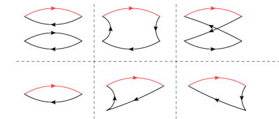
Figure 1: Diagrams showing the quark contractions for the entries of our correlation matrices for $\pi\pi$ and $K\pi$ scattering. The red propagator denotes a strange quark for $K\pi$ and a light one for $\pi\pi$, while the black propagators are for light quarks in both cases. The top row shows contractions for $2\to 2$ particle correlators. The right-most diagram does not appear for $I=1$ $\pi\pi$ scattering, but is required for our $K\pi$ scattering calculation. The second row contains $1\to 1$, $2\to 1$ and $1\to 2$ entries, respectively, where the $1\to 2$ element is the complex conjugate of $2\to 1$.

In $K\pi$ scattering, the $K^{*}$ resonance is in the $I=1/2$ channel, so we use

$$\pi(\mathbf{p}_{1})K(\mathbf{p}_{2})=\sqrt{\frac{2}{3}}\pi^{+}(\mathbf{p}_{1})K^{-}(\mathbf{p}_{2})-\sqrt{\frac{1}{3}}\pi^{0}(\mathbf{p}_{1})K^{0}(\mathbf{p}_{2})$$ (5)

as the two-particle interpolator. The one-particle interpolators are the same as for the $\rho$ resonance, replacing one light quark by the strange. From these interpolators we calculate a matrix of correlation functions. The contractions for its entries are depicted in Fig. 1.

Table 2: The interpolators we use in different moving frames. For each frame, we note the little group and irreducible representations (irrep) we employ and the one- and two-particle interpolators that belong to them. $\mathbf{K}$ denotes the integer valued total momentum vector (used for the one-particle interpolator) and the arguments of the pseudoscalar interpolators are $\mathbf{k}_{j}=\mathbf{p}_{j}L/(2\pi)$.

$\pi\pi$
$N_{s}$	$\mathbf{K}$	(Little) group	Irrep	$\mathcal{O}_{\pi\pi}$	$\mathcal{O}_{\rho}$
48	$(0,0,0)$	$O_{h}$	$T_{1}$	$\pi(1,0,0)\pi(-1,0,0)$	$\rho_{x}$
48	$(0,0,1)$	$C_{4v}$	$E$	$\pi(1,0,0)\pi(-1,0,1)-\pi(-1,0,0)\pi(1,0,1)$	$\rho_{x}$
48	$(0,1,1)$	$C_{2v}$	$A_{1}$	$\pi(1,0,0)\pi(-1,1,1)+\pi(-1,0,0)\pi(1,1,1)$	$\rho_{y}+\rho_{z}$
48	$(0,1,1)$	$C_{2v}$	$B_{1}$	$\pi(1,0,0)\pi(-1,1,1)-\pi(-1,0,0)\pi(1,1,1)$	$\rho_{x}$
64	$(0,0,1)$	$C_{4v}$	$E$	$\pi(1,0,0)\pi(-1,0,1)-\pi(-1,0,0)\pi(1,0,1)$	$\rho_{x}$
64	$(0,1,1)$	$C_{2v}$	$A_{1}$	$\pi(1,0,0)\pi(-1,1,1)+\pi(-1,0,0)\pi(1,1,1)$	$\rho_{y}+\rho_{z}$
64	$(0,1,1)$	$C_{2v}$	$B_{1}$	$\pi(1,0,0)\pi(-1,1,1)-\pi(-1,0,0)\pi(1,1,1)$	$\rho_{x}$
$K\pi$
$N_{s}$	$\mathbf{K}$	(Little) group	Irrep	$\mathcal{O}_{K\pi}$	$\mathcal{O}_{K^{*}}$
48	$(1,1,0)$	$C_{2v}$	$B_{2}$	$\pi(1,0,0)K(0,1,0)$	$K^{*}_{x}-K^{*}_{y}$
64	$(0,0,0)$	$O_{h}$	$T_{1}$	$\pi(1,0,0)K(-1,0,0)$	$K^{*}_{x}$
64	$(0,0,1)$	$C_{4v}$	$E$	$\pi(1,0,0)K(-1,0,1)-\pi(-1,0,0)K(1,0,1)$	$K^{*}_{x}$
64	$(0,1,1)$	$C_{2v}$	$A_{1}$	$\pi(1,0,0)K(-1,1,1)+\pi(-1,0,0)K(1,1,1)$	$K^{*}_{y}+K^{*}_{z}$
64	$(0,1,1)$	$C_{2v}$	$B_{1}$	$\pi(1,0,0)K(-1,1,1)-\pi(-1,0,0)K(1,1,1)$	$K^{*}_{x}$

By using the two volumes and a number of moving frames, we are able to access several points within the regions of interest around the expected positions of the $\rho$ and $K^{*}$ resonances. The kinematic points we use are given in Table 2, where

$$\mathbf{K}=\frac{L}{2\pi}\mathbf{P}$$ (6)

denotes an integer-valued lattice momentum vector. The choice of momenta and representations is based on the requirement that the non-interacting two-particle states lie within or close to the expected resonance widths. To allow reuse of the generated propagators, we restrict ourselves to $\mathbf{k}_{1}=\mathbf{p_{1}}L/(2\pi)=(1,0,0)$. For each total momentum $\mathbf{P}$, we have to construct interpolators which transform according to a definite irreducible representation (irrep) of the little group of allowed cubic rotations once a Lorentz boost has been applied. We construct the interpolators using the information about the little groups given in Ref. Göckeler et al. (2012). The irreps we work with and the (one- and two-particle) interpolators that transform according to each representation are also listed in Table 2. We use Schoenflies notation (see, for example, Ref. Hamermesh (1962)) for the names of the groups and irreps.

The necessary quark line contractions are depicted in Fig. 1, where the first row includes two-particle to two-particle transitions and the second row one- to one- as well as two- to one-meson transitions. We use stochastic $\mathbb{Z}_{2}+i\mathbb{Z}_{2}$ wall sources at one time slice for each spin component and, for the contractions involving the two-particle interpolators, sequential inversions to generate all the contributing diagrams, following Refs. Aoki et al. (2007, 2011). To compute the top left contraction of Fig. 1, it is necessary to use two stochastic sources per configuration. We use this minimum number of estimates per configuration as the gauge noise dominates. We further reduce the computational cost by fixing $\mathbf{k}_{1}$ to $(1,0,0)$. Even with this restriction, we can obtain several interesting levels around the expected positions of the $\rho$ and $K^{*}$ resonances. Moreover, we only compute the full $\pi\pi\to\pi\pi$ correlator from $t=6a$ to $t=17a$, where we anticipate that on one hand the signal is only moderately polluted by excited state contributions and on the other hand statistical errors are still tolerable. We are also able to “recycle” many propagators in both $\pi\pi$ and $K\pi$ scattering.

Adding this up, in our implementation the total number of solves required on each configuration is

$$N_{\mathrm{vec}}\left[N_{\mathrm{smear}}+N_{p_{1}}(1+18N_{p_{2}}+3N_{\mathrm{times}})\right]\,,$$ (7)

where $N_{\mathrm{vec}}=8$ is the number of noise sources used (four spin components times two different vectors), $N_{\mathrm{smear}}=4$ is the number of one-particle smearing levels (three plus one derivative source, see above), $N_{p_{1}}=1$ and $N_{p_{2}}$ (see Table 2) are the numbers of momenta calculated and $N_{\mathrm{times}}=12$ ($t=6a$ up to $t=17a$) is the number of time slices for which the box diagrams shown in the top middle and top right of Fig. 1 are calculated. For the $N_{s}=48$ and $N_{s}=64$ lattices, evaluating the full eight by eight matrices of correlators for each moving frame amounts to inverting the strange quark Wilson matrix 80 and 120 times, respectively, and the light quark matrix 824 and 808 times. Note that the number of solves required to compute a “traditional” point-to-all propagator is twelve, i.e. the present scattering computation is by a factor of about $40$ more expensive than a conventional determination of the spectrum of stable light hadrons for one quark smearing level (twelve strange and twelve light quark inversions on each volume).

The momenta injected are not indicated in Fig. 1 and the correlator is the sum of all allowed momentum projections; some irreps require a combination of two related pairs of momenta and, in $\pi\pi$ scattering, we can interchange the momenta $\mathbf{p}_{1}$ and $\mathbf{p}_{2}$ carried by each pion at the sink. Similarly, we ensure that the one-particle to one-particle correlators — depicted in the lower left of the figure — transform according to the irreps given in Table 2, by taking the corresponding combinations of vector meson polarizations. The contractions for $\pi\pi\to\rho$ and $\rho\to\pi\pi$ are complex conjugates and it is computationally cheaper to only calculate one of them. (We do this for $\pi\pi\to\rho$.) For the remaining correlation matrix elements with $i\neq j$ (one- to one-particle), we average over $C_{ij}$ and $C^{*}_{ji}$.

II.3 Extraction of energy levels and phase shifts

For each kinematic situation, we construct an eight times eight matrix of correlators for our basis of interpolators in the way described above. The element of this matrix for a source interpolator $\mathcal{O}_{j}$ and a sink interpolator $\mathcal{O}_{i}$ is given as

$$C_{ij}(t)=\langle 0|\hat{\mathcal{O}}_{i}(t)\hat{\mathcal{O}}_{j}^{\dagger}(0)|0\rangle\,.$$ (8)

The spectral decomposition can be written as

$$C_{ij}(t)=\sum_{\alpha}\frac{Z^{i}_{\alpha}Z^{j*}_{\alpha}}{2E^{\alpha}}e^{-E^{\alpha}t}\,,$$ (9)

where $Z_{\alpha}^{i}=\langle 0|\hat{\mathcal{O}}_{i}|\alpha\rangle$ is the overlap factor of the state created by the operator $\hat{\mathcal{O}}_{i}^{\dagger}$ with the physical state $|\alpha\rangle$ of energy $E^{\alpha}$. We extract the energy levels $E^{\alpha}$ by solving the generalized eigenvalue problem Michael (1985); Lüscher and Wolff (1990); Blossier et al. (2009)

$$C(t)u^{\alpha}(t)=\lambda^{\alpha}(t_{0},t)C(t_{0})u^{\alpha}(t)\,,$$ (10)

where the energy levels can be obtained from the dependence $\lambda^{\alpha}(t_{0},t)\sim e^{-E^{\alpha}(t-t_{0})}$ at large times.

The energies we extract are in the lab frame, so we denote these as $E_{L}$. The phase shift, however, is extracted in the centre of momentum frame, i.e. in the rest frame of the $\pi\pi$- or $\pi K$-system. It is straightforward to convert the lab frame energies $E_{L}$ into the corresponding centre of momentum frame energies $E_{cm}$.

The lab frame energy of the two-meson state is given as

$$E_{L}=\sqrt{\mathbf{p}_{1}^{2}+m_{1}^{2}}+\sqrt{\mathbf{p}_{2}^{2}+m_{2}^{2}}\,,$$ (11)

where the $m_{i}$ are the pion (or kaon) masses and the $\mathbf{p}_{i}$ their momenta. In the absence of interactions the $\mathbf{p}_{i}^{2}$ are integer multiples of $(2\pi/L)^{2}$. The invariant squared energy in the centre of momentum frame is

$$E_{cm}^{2}=E_{L}^{2}-\mathbf{P}^{2}\,,$$ (12)

where $\mathbf{P}$ is the total momentum of the $\pi\pi$ (or the $K\pi$) system. The square of the momentum of each of the pseudoscalars in the centre of momentum frame is given by

$$p_{cm}^{2}=\frac{\left(E_{cm}^{2}-(m_{1}+m_{2})^{2}\right)\left(E_{cm}^{2}-(m_{1}-m_{2})^{2}\right)}{4E_{cm}^{2}}\,.$$ (13)

The phase shift is extracted, comparing the centre of momentum frame spectrum to the energy levels allowed by the residual cubic symmetry (little group) that corresponds to the boost applied. For each irrep, this involves an expression in terms of generalized zeta functions, derived in Refs. Leskovec and Prelovsek (2012); Göckeler et al. (2012). For the numerical calculation of these functions, we use the representation given in Ref. Göckeler et al. (2012).

The generalized zeta function is a function of the real-valued variable $q=p_{cm}L/(2\pi)$:

$$Z_{\ell m}(q^{2})=\sum_{\mathbf{z}}\frac{\mathcal{Y}_{\ell m}(\mathbf{z})}{\mathbf{z}^{2}-q^{2}}\,,$$ (14)

where $\mathcal{Y}_{\ell m}(\mathbf{z})=|\mathbf{z}|^{\ell}Y_{\ell m}(\mathbf{e}_{z})$ with $\mathbf{e}_{z}=\mathbf{z}/|\mathbf{z}|$ and $Y_{\ell m}$ are the usual spherical harmonics. The sum is over $\mathbf{z}$, the allowed momentum vectors in the boosted frame, see, e.g., Ref. Göckeler et al. (2012).

For each irrep we have to consider mixing between different continuum partial waves. The relevant determinants from which the phase shifts can be extracted are listed in Ref. Göckeler et al. (2012). Here, we neglect possible mixing with partial waves $\ell\neq 1$. The $s$-wave can only contribute to $K\pi$ scattering. Moreover, mixing of $\ell=0$ into $\ell=1$ is only allowed for the $\mathbf{K}=(0,1,1)$ $A_{1}$ irrep. We will address this case in Sec. III.3 below. Since the $\pi\pi$ and $K\pi$ interactions have a finite range, contributions of higher partial waves are suppressed. The $\ell=3$ $\pi\pi$ phase shift was determined recently by Wilson and collaborators Wilson et al. (2015a) at $m_{\pi}\approx 236\,\textmd{MeV}$ who indeed found $\delta_{3}\approx 0$ near the resonance, within small errors. We conclude that limiting ourselves to $\ell\leq 1$ appears reasonable.

Subsequently, we parameterize the phase shift as a function of the centre of momentum frame energy using a Breit-Wigner (BW) ansatz:

$$\tan\delta=\frac{g^{2}}{6\pi}\frac{p_{cm}^{3}}{E_{cm}(m_{R}^{2}-E_{cm}^{2})}\,.$$ (15)

From this parametrization, we can extract the mass of the resonance $m_{R}$ and its width can be found from the coupling $g$ as

$$\Gamma=\frac{g^{2}}{6\pi}\frac{p_{R}^{3}}{m_{R}^{2}}\,,$$ (16)

where $p_{R}$ is the momentum carried by each particle in the centre of momentum frame at $\delta=\pi/2$, i.e. $p_{R}$ is given by $p_{cm}$ of Eq. (13) for $E_{cm}=m_{R}$.

III Results

III.1 Determination of the energy levels

Following the generalized eigenvalue procedure detailed in Sec. II.3 above, we separately analyse the eight by eight matrices that cross-correlate states created by one- and two-particle interpolators for the seven $\pi\pi$ and five $K\pi$ channels listed in Table 2, and obtain the respective ground and first excited state energies. We are able to resolve these energies most easily using sub-matrices of correlators containing only three interpolators — one of which always is the two-particle interpolator $\mathcal{O}_{\pi\pi}$ or $\mathcal{O}_{K\pi}$ of Table 2. The single-particle interpolators used in the final analysis are only of the type $\bar{\psi}\gamma_{j}\psi$. However, we have checked these results against employing other sub-matrices and found consistency of the effective masses, but no improvement. The results turned out very similar but often noisier when replacing one $\bar{\psi}\gamma_{j}\psi$ interpolator by $\bar{\psi}\gamma_{j}\gamma_{t}\psi$ while the $\bar{\psi}\nabla_{j}\psi$ interpolator increased the statistical errors very significantly, in particular for states with total momentum $\mathbf{K}=(0,1,1)$.

To save computer time we only evaluated the box diagrams in the top middle and top right of Fig. 1 for $17a\geq t\geq 6a$. The top left diagram contains two traces and naively increases like $L^{6}$ while the quark-line connected box diagrams have magnitudes $\propto L^{3}$. Due to this relative suppression, these can only become important at times of at least a similar magnitude as the inverse energy gap between $I=2$ and $I=1$ $\pi\pi$ (or $I=3/2$ and $I=1/2$ $K\pi$) states and probably their contribution to the $\pi\pi\to\pi\pi$ and $K\pi\to K\pi$ entries can be neglected at $t<6a$. Nevertheless, to be on the safe side, in our generalized eigenvector analysis we set $t_{0}=6a\approx 0.43\,\textmd{fm}$.

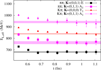
Figure 2: Effective masses for some $\pi\pi$ and $K\pi$ channels. The error bands correspond to the fit results.

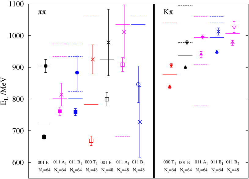
Figure 3: Energy levels of the $\rho|\pi\pi$ (left) and $K^{*}|K\pi$ (right) systems in finite boxes of linear sizes $N_{s}a=48a\approx 2.6/m_{\pi}^{\infty}\approx 3.4\,\textmd{fm}$ and $N_{s}a=64a\approx 3.5/m_{\pi}^{\infty}\approx 4.6\,\textmd{fm}$ for different lattice momenta and representations in the laboratory frame. Horizontal lines correspond to the energy levels of a non-interacting two-particle system. Squares and upward pointing triangles indicate ground states, circles and downward pointing triangles first excited states. Open symbols correspond to the smaller volume and full symbols to the larger volume. Crosses are for levels that are not used in our subsequent phase shift analysis. Note that for $\pi\pi$ scattering the excited states in both $\mathbf{K}=(0,0,1)$ $E$ channels are above the respective non-interacting $4\pi$ thresholds (not shown).

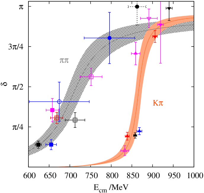
Figure 4: The phase shift as a function of the centre of momentum frame energy, $E_{cm}$, for $p$-wave $\pi\pi$ scattering around the $\rho$ resonance and $K\pi$ scattering around the $K^{*}$ resonance. The data correspond to the lab frame energies shown in Fig. 3, with matched colours and symbols. The curves with error bands are Breit-Wigner parametrizations. The dashed error bar indicates a point in $\pi\pi$ scattering which lies above the four-pion threshold.

We show effective masses

$$E_{L,\mathrm{eff}}^{\alpha}(t+a/2)=\frac{1}{a}\ln\frac{\lambda^{\alpha}(t_{0}=6a,t)}{\lambda^{\alpha}(t_{0}=6a,t+a)}$$ (17)

for some of our $\pi\pi$ and $K\pi$ eigenvalues, see Eq. (10), in Fig. 2, for the region $t>t_{0}+a$. To enable better comparison to other studies, we display the data in physical units. The effective masses are typically consistent with plateaus between $t=10a\approx 0.71\,\textmd{fm}$ and $17a\approx 1.22\,\textmd{fm}$, which is our most frequent fit range, although there are differences between the channels. The $K\pi$ $T_{1}$ channel shown in the figure is an extreme example, where the fit range starts at $t=14a\approx 1\,\textmd{fm}$.

Of particular interest are the $\mathbf{K}=(0,1,1)$ $A_{1}$ channels. The non-interacting ground states in this irrep correspond to a momentum distribution $\mathbf{k}_{1}=\bf{0}$ and $\mathbf{k}_{2}=\mathbf{K}=(0,1,1)$ among the two pseudoscalar mesons that differs from the one used in constructing our two-particle interpolators ($\mathbf{k}_{1}=(1,0,0)$ and $\mathbf{k}_{2}=\mathbf{K}-\mathbf{k}_{1}=(-1,1,1)$). In principle, these correlation functions could decay towards the lower lying states. However, we find no indication for this in our data, see Fig. 2, and conclude that our interpolators effectively decouple from these energy levels.

The resulting lab frame energy levels $E_{L}$ are shown in Fig. 3 both for the $\pi\pi$ and $K\pi$ channels. The scale is set using $a^{-1}=2.76\,\textmd{GeV}$, ignoring the 3% overall scale uncertainty for the moment being. The statistical errors are obtained using the jackknife procedure. Only two $\pi\pi$ levels are above the four-pion threshold (the excited states in the $\mathbf{K}=(0,0,1)$ $E$ irrep), one of which will be disregarded in any case in the phase shift analysis below.

In the figure, we also show the energies of the non-interacting two-particle states. The solid horizontal lines are the non-interacting levels corresponding to the two-particle interpolators explicitly included in our basis (given in Table 2), while the dashed lines correspond to other distributions of the momentum among the non-interacting pseudoscalar mesons. As we have not included interpolators that explicitly resemble these momentum configurations, we cannot rely on our extracted energy levels to be sensitive to their presence and ignore these non-interacting levels in our phase shift analysis. As already discussed above, in the $A_{1}$ case the non-interacting ground states are lower in energy than the levels that correspond to the momentum distribution we have implemented (solid lines). Nevertheless, we see no evidence of any coupling of the interpolators within our basis to these states, see Fig. 2. Note that for the $N_{s}=64$ $\pi\pi$ channel this level lies at $561\,\textmd{MeV}$, below the energy region shown in Fig. 3.

Levels that are irrelevant, due to large statistical errors for the resulting phase shifts, will be excluded from our subsequent analysis. These levels are depicted as crosses in Fig. 3. We remind the reader that the deviations of the measured energy levels shown in the figure from the non-interacting two-particle levels (solid lines) are due to the $\rho$ and $K^{*}$ resonances and encode the resonance parameters.

III.2 Phase shift and resonance parameters

The centre of momentum frame energies $E_{cm}$ and phase shifts $\delta(E_{cm})$ can both be extracted from measured lab frame energy levels $E_{L}$ in a given irrep, see Sec. II.3, where we assume $m_{\pi}=149.5\,\textmd{MeV}$, in spite of the fact that the measured pion mass on the small volume is larger by $10\,\textmd{MeV}$. This will be addressed in Sec. III.3 below.

We plot $\delta(E_{cm})$ in Fig. 4, using the same colour and symbol scheme as in Fig. 3. As explained above, in our determination of the phase shift we assume that one value of $\ell$ ($\ell=1$) dominates, such that there is a one to one correspondence between the extracted energy levels and the points in the phase shift curves. For clarity we omit all data points from the figure with errors on the phase shift in excess of $\pi/5$ (marked as crosses in Fig. 3). These have little statistical impact and will therefore be excluded from our analysis.

The $\pi\pi$ and $K\pi$ phase shifts are each fitted to the BW resonance form given in Eq. (15). Our fit to the $\pi\pi$ phase shift results in $\chi^{2}/\mathrm{d.o.f}=8.9/7$ and for the $K\pi$ phase shift we obtain $\chi^{2}/\mathrm{d.o.f.}=19.2/7$. These fits are included in Fig. 4 (the grey hashed band for $\pi\pi$ scattering and the solid orange one for $K\pi$ scattering). In the $\pi\pi$ case the dashed data point of the figure is slightly above the respective $4\pi$ threshold. However, as discussed in the introduction, the effect of this inelastic threshold is expected to be negligible. Moreover, excluding this point from the fit only produces a hardly visible change. Since we have exact isospin symmetry in place, decays into three-pion final states are not possible.

Figures 3 and 4 clearly show an increase in statistical noise when going to smaller quark masses: The $\pi\pi$ scattering data have considerably larger error bars than the $K\pi$ data. From the BW fits shown, we find the values

$$m_{\rho}=716(21)(21)\,\textmd{MeV}\,, \quad m_{K^{*}}=868(8)(26)\,\textmd{MeV}\,,$$ (18)

$$g_{\rho\pi\pi}=5.64\pm 0.87\,, \quad g_{K^{*}K\pi}=4.79\pm 0.49\,,$$ (19)

$$\Gamma_{\rho}=113(35)(3)\,\textmd{MeV}\,, \quad\Gamma_{K^{*}}=30(6)(1)\,\textmd{MeV}\,,$$ (20)

for $\pi\pi$ and $K\pi$ scattering, where the first errors are statistical and the second errors reflect our 3% overall scale uncertainty Bali et al. (2013). In the last row we also quote the corresponding decay widths, obtained via Eq. (16). From a given parametrization of the $p$-wave phase shift, assuming partial wave unitarity and ignoring further inelastic thresholds, we can analytically continue to the second (unphysical) Riemann sheet (see, e.g., Ref. Burkhardt (1969)) and determine the position of the resonance pole. Using the BW parametrization, for the $\rho$ and $K^{*}$ resonances we find $\sqrt{s_{R}}=[707(17)-\mathrm{i}\,55(18)]\,\textmd{MeV}$ and $\sqrt{s_{R}}=[868(10)-\mathrm{i}\,14.4(3.4)]\,\textmd{MeV}$, respectively. These numbers are consistent with $\sqrt{s_{R}}=m_{R}-\mathrm{i}\,\Gamma/2$ from the BW fits Eqs. (18) and (20). Note, however, that $\textmd{Re}\sqrt{s_{\rho}}$ is by about half a standard deviation smaller than the BW fit parameter $m_{\rho}$. In Sec. III.3 we will explore in detail the parametrization dependence of these results.

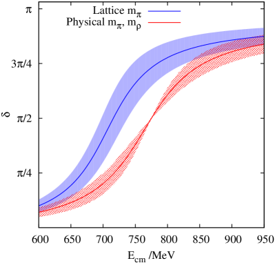
Figure 5: We compare phase shift curves for $\pi\pi$ scattering around the $\rho$ resonance for our fitted Breit-Wigner resonance (solid blue band) and one with the fitted coupling but physical pion and $\rho$ masses (hashed red band).

We emphasize that our study was carried out at a single lattice spacing only, which is not reflected in the errors given above. Both resonant masses come out smaller than the experimental values, $775\,\textmd{MeV}$ and $896\,\textmd{MeV}$, respectively. The reduced decay phase space, due to a 10% heavier than physical pion, in conjunction with somewhat smaller than physical resonance masses, is the main reason why our decay widths appear to be somewhat below the experimental ones, $\Gamma_{\rho}\approx 148\,\textmd{MeV}$ and $\Gamma_{K^{*}}\approx 47\,\textmd{MeV}$, although this difference is only statistically significant for the $K^{*}$. The coupling $g_{\rho\pi\pi}$ is consistent with the experimental value $g_{\rho\pi\pi}\approx 5.93$ while our $g_{K^{*}K\pi}$ is slightly lower than $g_{K^{*}K\pi}\approx 5.39$. The ordering $g_{\rho\pi\pi}>g_{K^{*}K\pi}$ is reproduced, albeit within large errors.

In Fig. 5 the $\pi\pi$ phase shift curve fitted to our data is compared to the same curve with the $\pi$ and $\rho$ masses set to their physical values Olive et al. (2014), but the coupling $g_{\rho\pi\pi}$ taken from our fit Eq. (19). The latter curve is forced to run through $\delta=\pi/2$ at the fixed resonant mass $E_{R}=E_{cm}=775\,\textmd{MeV}$ as we use the BW parametrization. Since our value of $g_{\rho\pi\pi}$ agrees with experiment, experimental data will be described by the hashed red band. Again, there is an overall scale setting uncertainty of 3% on $E_{cm}$, corresponding to $20\,\textmd{MeV}$, that we do not display as well as other systematics, most notably a 10% heavier than physical pion and a fixed lattice spacing. The figure illustrates that also in terms of the width of the resonance we are close to the physical case. Previous studies of $\pi\pi$ scattering have not directly addressed the physical limit, although unitarized chiral perturbation theory has been used in Ref. Bolton et al. (2015) to extrapolate lattice data obtained at $m_{\pi}\approx 236\,\textmd{MeV}$ Wilson et al. (2015a) to the physical point.

III.3 Investigation of possible biases

Here we investigate the effects on the extracted resonance parameters, of the finite volume pion mass shift, of the BW parametrization we use to fit $\delta(E_{cm})$ and of the presence of inelastic thresholds. We also address the possibility of an $\ell=0$ pollution for the case of $K\pi$ scattering.

The pion mass enters the generalized zeta function, Eq. (14), via the calculation of the momentum carried by the two particles in the centre of momentum frame, given by Eq. (13). We prefer to use the infinite volume pion and kaon masses throughout because we are relating the spectra to scattering amplitudes in an infinite volume. For the larger $L=64a$ lattice size, the pion mass determined in the finite volume and that extrapolated to infinite volume differ by as little as $0.2\,\textmd{MeV}$ Bali et al. (2014). However, the pion mass measured on the $L=48a$ configurations differs from the infinite volume mass by $10\,\textmd{MeV}$ and the kaon mass by $3\,\textmd{MeV}$. Since pion exchanges around the boundaries of the periodic box go beyond the Lüscher formalism, we have repeated the analysis using finite volume pion masses instead, to explore these systematics. For the $L=64a$ data the effect obviously is insignificant. For $L=48a$ the phase shifts for the corresponding six points (four for the $\rho$ resonance and two for $K^{*}$) depicted in Fig. 4 (open symbols) increase by values ranging from $0.03$ to $0.05$. These differences are considerably smaller than our errors on $\delta$. Indeed, using these numbers instead, we find the $\rho$ and $K^{*}$ resonance parameters $m_{\rho}=713(18)\,\textmd{MeV}$, $m_{K^{*}}=867(7)\,\textmd{MeV}$, $g_{\rho\pi\pi}=5.56(85)$ and $g_{K^{*}K\pi}=4.81(51)$, in almost perfect agreement with our main analysis employing the infinite volume pion mass Eqs. (18) and (19). For instance, the central values for the masses deviate by only $-3\,\textmd{MeV}$ and $-1\,\textmd{MeV}$, respectively. Adding these systematics to the statistical errors in quadrature has no impact.

Table 3: $\rho$ resonance: fit results for various phase shift models. The square root of the resonance pole position $s_{R}$ may be used to define $\sqrt{s_{R}}=m_{R}-\frac{\mathrm{i}}{2}\,\Gamma_{R}$. The errors given are statistical only.

Model	$m_{\rho}/\textmd{MeV}$	$g_{\rho\pi\pi}$	other fit parameters	$\sqrt{s_{R}}/\textmd{MeV}$
0: Eq. (15) (BW)	716(21)	5.64(87)	—	$707(17)-\frac{\mathrm{i}}{2}\,110(36)$
1: Eq. (22)	717(23)	5.38(84)	$R=3(6)\,\textmd{GeV}^{-1}$	$714(26)-\frac{\mathrm{i}}{2}\,104(35)$
2: Eq. (23)	718(23)	5.34(84)	$\beta=0.16(15)\,\textmd{GeV}$	$716(29)-\frac{\mathrm{i}}{2}\,103(35)$
3: Eq. (24)	717(23)	—	$B_{0}=1.31(45)$, $B_{1}=1.6(3.0)$	$714(26)-\frac{\mathrm{i}}{2}\,103(37)$

Table 4: $K^{*}$ resonance: fit results for various phase shift models, including and excluding the two $\mathbf{K}=(0,1,1)$ $A_{1}$ irrep points that may also couple to the $\ell=0$ partial wave. The errors given are statistical only.

Model	$A_{1}$ included	$m_{K^{*}}/\textmd{MeV}$	$g_{K^{*}K\pi}$	other fit parameters	$\sqrt{s_{R}}/\textmd{MeV}$
0: Eq. (15) (BW)	yes	868(8)	4.79(49)	—	$866(7)-\frac{\mathrm{i}}{2}\,30(7)$
1: Eq. (22)	yes	868(9)	4.78(44)	$R=6(29)\,\textmd{GeV}^{-1}$	$868(9)-\frac{\mathrm{i}}{2}\,30(7)$
2: Eq. (23)	yes	868(9)	4.80(47)	$\beta=0.13(45)\,\textmd{GeV}$	$867(10)-\frac{\mathrm{i}}{2}\,30(8)$
3: Eq. (24)	yes	868(9)	—	$B_{0}=3.2(5.3)$, $B_{1}=8.2(28.9)$	$868(10)-\frac{\mathrm{i}}{2}\,29(7)$
0: Eq. (15) (BW)	no	873(9)	5.08(43)	—	$871(8)-\frac{\mathrm{i}}{2}\,35(7)$
1: Eq. (22)	no	878(10)	5.09(38)	$R=1.2(1.6)\,\textmd{MeV}^{-1}$	$877(10)-\frac{\mathrm{i}}{2}\,36(6)$
2: Eq. (23)	no	887(7)	4.42(69)	$\beta=58(13)\,\textmd{MeV}$	$890(7)-\frac{\mathrm{i}}{2}\,27(9)$
3: Eq. (24)	no	886(8)	—	$B_{0}=10(5)$, $B_{1}=44(25)$	$888(9)-\frac{\mathrm{i}}{2}\,24(6)$

Next, we replace the BW parametrization of the scattering phase shift, see Eq. (15), by other functional forms suggested in Ref. Dudek et al. (2013) and references therein. We write,

$$\tan\delta=\frac{E_{cm}\Gamma(E_{cm})}{m_{R}^{2}-E_{cm}^{2}}\,,\quad\Gamma^{(0)}(E_{cm})=\frac{g^{2}}{6\pi}\frac{p_{cm}^{3}}{E_{cm}^{2}}\,,$$ (21)

where $\Gamma=\Gamma(m_{R})$ is the resonance width and the energy dependent width function $\Gamma(E_{cm})$ equals $\Gamma^{(0)}(E_{cm})$ in the BW case. In addition, we use von Hippel and Quigg (1972); Li et al. (1994); Peláez. and Yndurain (2005)

$$\Gamma^{(1)}(E_{cm}) =\frac{g^{2}}{6\pi}\frac{p_{cm}^{3}}{E_{cm}^{2}}\frac{1+(p_{R}R)^{2}}{1+(p_{cm}R)^{2}}\,,$$ (22)

$$\Gamma^{(2)}(E_{cm}) =\frac{g^{2}}{6\pi}\frac{p_{cm}^{3}}{E_{cm}^{2}}\exp\left(\frac{p^{2}_{R}-p^{2}_{cm}}{6\beta^{2}}\right)\,,$$ (23)

$$\Gamma^{(3)}(E_{cm}) =2\frac{p_{cm}^{3}}{E_{cm}^{2}}$$ (24)

$$\times \quad\left(B_{0}+B_{1}\frac{E_{cm}-\sqrt{s_{0}-E_{cm}^{2}}}{E_{cm}+\sqrt{s_{0}-E_{cm}^{2}}}\right)^{\!\!-1}\!\!\!\!,$$

where $s_{0}=(2m_{\pi}+m_{R})^{2}$. The BW fit function depends on two fit parameters, the resonant mass $m_{R}$ and the coupling $g$, while the other parametrizations depend on three parameters: $\Gamma^{(1)}$ contains the additional parameter $R$, $\Gamma^{(2)}$ contains $\beta\sim 1/(\sqrt{6}R)$ and $g$ is replaced by $B_{0}$ and $B_{1}$ within $\Gamma^{(3)}$.

Our fit results for $\pi\pi$ scattering are shown in Table 3. In all cases the additional parameter ($R$, $\beta$ and $B_{1}$) turned out to be consistent with zero. All the resonant masses we obtain are in perfect agreement with the BW result shown in the first row. Also the widths are compatible with the BW width $\Gamma^{(0)}=113(35)\,\textmd{MeV}$ of Eq. (20) and the parameter $B_{0}=1.31(45)$ is consistent with the expectation $B_{0}\approx 1.07$, extracted from experimental data in Ref. Peláez. and Yndurain (2005). Interestingly, we observe the numerically biggest difference (half a standard deviation) between the energy at a phase shift $\delta=\pi/2$, $m_{\rho}=E_{cm}(\pi/2)$, and the real part of $\sqrt{s_{R}}$ for the BW parametrization. We conclude from Table 3 that within our precision, we can neither differentiate between the different models nor distinguish the pole position in the second Riemann sheet from the naively fitted mass and width.

In our determination of the $\pi\pi$ energy levels, we noted that there was one data point above the four-pion threshold (the dashed point of Fig. 4). Excluding this from any of our four fits, however, had no impact worthy of mentioning.

For $K\pi$ scattering, in the case of the $\mathbf{K}=(0,1,1)$ $A_{1}$ irrep, we cannot exclude the possibility of a $\ell=0$ partial wave admixture. Therefore, we perform all fits (setting $s_{0}=(m_{\pi}+m_{K}+m_{R})^{2}$ in Eq. (24)) including and excluding the corresponding two data points, see the pink solid triangles in Figs. 3 and 4. The resulting fit parameters and the position of the $K^{*}$ pole are displayed in Table 4. When including the two $A_{1}$ points, there is no sensitivity to the additional fit parameters and all the results are remarkably stable. Including and excluding these points, real and $2\mathrm{i}$ times the imaginary part of $\sqrt{s_{R}}$ perfectly agree with the fitted masses and widths obtained through Eqs. (21)–(24), as one would expect for $\Gamma_{K^{*}}/m_{K^{*}}\approx 0.035\ll 1$. Removing the two points, however, appears to increase the resonant mass. Also the fit results become less stable since the BW fit has only five remaining degrees of freedom while the other three fits have only four.

In conclusion, while we find $g_{K^{*}K\pi}$ to be very stable against variations of the parametrization and of the number of points fitted, the $K^{*}$ mass is somewhat affected by the latter. Therefore, we allow for another systematic error of $10\,\textmd{MeV}$ to be added to the statistical error shown in Eq. (18) in quadrature:

$$m_{K^{*}}=868(13)(26)\,\textmd{MeV}\,.$$ (25)

III.4 Investigation of an alternative method

It is possible to estimate the value of the coupling $g_{\rho\pi\pi}$ directly from the correlators, using the McNeile-Michael-Pennanen (MMP) method introduced in Refs. McNeile et al. (2002); McNeile and Michael (2003) (also see Refs. Gottlieb et al. (1984, 1986) for earlier, related work), if the momentum and volume are selected such that the $\pi\pi$ energy is close to the resonant mass $m_{\rho}=m_{R}$. This method was also employed recently for studying the $\Delta$ resonance Alexandrou et al. (2013).

Using the correlators defined in Eq. (8), with $\mathcal{O}_{1}$ and $\mathcal{O}_{2}$ being two- and one-particle interpolators, we can extract (approximate) ground state energies $E_{\pi\pi}$ and $E_{\rho}$ from $C_{11}(t)$ and $C_{22}(t)$ alone, respectively, at times sufficiently small to avoid the higher level to decay into the lower level (if $E_{\rho}\neq E_{\pi\pi}$) and large enough for excited state contributions to be negligible. In this situation, the ground state contribution to $C_{12}(t)$ reads

$$C_{12}(t)\approx xa\sum_{t^{\prime}}\frac{Z_{\pi\pi}^{1}Z_{\rho}^{2*}}{2\sqrt{E_{\pi\pi}E_{\rho}}}e^{-E_{\pi\pi}(t-t^{\prime})}e^{-E_{\rho}t^{\prime}}\,,$$ (26)

where $Z_{\alpha}^{i}$ are the amplitudes to create the states $|\alpha\rangle$ using $\hat{\mathcal{{O}}}^{\dagger}_{i}$. These overlap factors also appear within $C_{11}(t)$ and $C_{22}(t)$ [see Eq. (9)] and will cancel as we are going to divide $C_{12}$ by an appropriate combination of these two elements in Eqs. (28) and (29) below. The $\rho$ state created at $t=0$ will propagate to a time $t^{\prime}<t$, where it undergoes a transition into $\pi\pi$. $x$ is the associated $\rho\to\pi\pi$ transition amplitude and in Eq. (26) we summed over all possible intermediate times $t^{\prime}$. The underlying assumption is that the overlaps of $\hat{\mathcal{O}}_{2}^{\dagger}|0\rangle$ with $|\pi\pi\rangle$ and of $\hat{\mathcal{O}}_{1}^{\dagger}|0\rangle$ with $|\rho\rangle$ are small and can be treated as perturbations, at least if $t$ is not taken too large. Obviously, there are corrections of higher order in $x$ to Eq. (26).

The coupling $g_{\rho\pi\pi}$ can then be estimated from $x$ through McNeile and Michael (2003)

$$g^{2}_{\rho\pi\pi}\approx\frac{L^{3}E_{cm}^{3}}{4p_{cm}^{2}}|x|^{2}\,.$$ (27)

This can be seen as follows McNeile and Michael (2003). Fermi’s Golden Rule relates the decay width to the matrix element $x$ in the centre of momentum frame: $\Gamma\approx|x|^{2}L^{3}p_{cm}E_{cm}/(24\pi)$. This can be re-expressed in terms of $g^{2}$ through $\Gamma=g^{2}p_{cm}^{3}/(6\pi E_{cm}^{2})$, see Eq. (16), where $E_{cm}$ is taken at the point $\delta=\pi/2$. The prefactor $L^{3}p_{cm}E_{cm}/(24\pi)$ above contains the following contributions: $2\pi$ from the Golden Rule, $L^{3}p_{cm}E_{cm}/(8\pi^{2})$ from the density of states, $1/2$ for a decay into identical pions and $1/3$, averaging over one pion momentum direction for the fixed $\rho$ polarization and momentum.

In Eq. (27) several assumptions have been made: (1) The Golden Rule is applicable, i.e. the $\pi\pi$ contribution to the initial $\rho$ meson state is insubstantial and the matrix element is not too large: $|x|t\ll 1$. This is synonymous with neglecting terms of higher order in $x$. (2) The volumes are sufficiently large for continuous density of states methods to be applicable. (3) The $\pi\pi$ and $\rho$ states have a similar energy and, in the centre of momentum frame, this is close to the resonant mass. (4) $x$ does not change substantially when transforming it from the lab to the centre of momentum frame.

Table 5: Estimates of $x$ and $g_{\rho\pi\pi}$ using the MMP method McNeile et al. (2002); McNeile and Michael (2003). The entries are sorted in terms of a descending gap $\Delta E=E_{\pi\pi}-E_{\rho}$. In the last row we show our result Eq. (19) from the Lüscher-type scattering analysis for comparison.

$N_{s}$	$\mathbf{K}$	Irrep	$\Delta E/\textmd{MeV}$	$x/\textmd{MeV}$	$g_{\rho\pi\pi}$
$48$	$(0,1,1)$	$A_{1}$	135	81(5)	5.54(30)
$48$	$(0,1,1)$	$B_{1}$	95	106(7)	7.07(44)
$48$	$(0,0,1)$	$E$	16	124(6)	8.37(39)
$48$	$(0,0,0)$	$T_{1}$	-35	113(4)	7.54(28)
$64$	$(0,1,1)$	$A_{1}$	-122	51(2)	5.19(17)
$64$	$(0,1,1)$	$B_{1}$	-140	73(3)	8.18(22)
$64$	$(0,0,1)$	$E$	-173	81(2)	7.46(25)
Full scattering analysis			—	—	5.64(87)

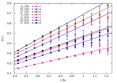
Figure 6: The ratio of correlators $R(t)$ defined in Eq. (29) for different irreps on the two volumes, see Table 5, together with linear fits to the first seven data points shown.

In the limit $E_{\pi\pi}=E_{\rho}$, summing over the intermediate time $t^{\prime}$, the ground state contribution to Eq. (26) has the time dependence $t\,e^{-E_{\pi\pi}t}$, while excited states are suppressed by a power of $t$, relative to this. In this case, $x$ can be found from a ratio of correlators as

$$\frac{|C_{12}(t)|}{\sqrt{C_{11}(t)C_{22}(t)}}\approx\textmd{const.}+xt\,,$$ (28)

up to exponential corrections in $t$ that contribute at small times and neglecting higher powers of $xt$. Since only $|x|^{2}$ is relevant, above we defined $x$ as real and positive. When the difference $\Delta E=E_{\pi\pi}-E_{\rho}$ is non-zero, we can still perform the sum over $t^{\prime}$ in Eq. (26). In this case the time dependence of the ground state contribution is $a[\sinh(\Delta Et/2)/\sinh(\Delta Ea/2)]e^{-\bar{E}t}$ (see, e.g., Ref. Alexandrou et al. (2013)), where the average energy is defined as $\bar{E}=\frac{1}{2}(E_{\pi\pi}+E_{\rho})$. The ground state contribution of the ratio of correlators can again be used to extract $x$:

$$R(t)\equiv\frac{|C_{12}(t)|}{\sqrt{C_{11}(t)C_{22}(t)}}\frac{t\sinh(\Delta E\,a/2)}{a\sinh(\Delta E\,t/2)}\approx\textmd{const.}+xt\,,$$ (29)

where we estimate $\Delta E$ from the exponential decay of the ratio $C_{11}(t)/C_{22}(t)$ at large (but not too large) times.

We now proceed to estimate $g_{\rho\pi\pi}$ to assess the reliability of the MMP method. In Fig. 6 we show the resulting ratios $R(t)$, together with linear fits to the first seven data points, $6a\leq t\leq 12a$. The colour coding of the symbols corresponds to that of Fig. 3. The extracted slopes vary between $51\,\textmd{MeV}$ and $124\,\textmd{MeV}$ with the smaller slopes corresponding to the larger volume (full symbols), as one would expect from the naive scaling with $L^{-3/2}$ of the amplitude $x$ defined in Eq. (26). This scaling is also consistent with Eq. (27), where the combination $x^{2}L^{3}$ appears. For the largest slope $x\approx 124\,\textmd{MeV}$ and $t=12a\approx 0.86\,\textmd{fm}$, we obtain $xt\approx 0.54$. Indeed, around this Euclidean time higher order corrections in $xt$ become relevant, while for the large volume data sets, where the slopes are smaller, the linear behaviour persists for much longer. We see no indication of exponential corrections towards small times.

In Table 5 we show the results for $x$ and the derived couplings, where the errors are purely statistical. More details on the momenta and interpolators used can be found in Table 2. The entries of Table 5 are ordered in terms of decreasing $\Delta E$, where we find that a smaller $\Delta E$ corresponds to a smaller $E_{cm}$ (and a smaller phase shift $\delta$), see Fig. 4. Naively, the $T_{1}$ and $E$ irreps on the $N_{s}=48$ lattice should give the most reliable results as these are closest to the resonance and best matched in terms of a small $\Delta E$. However, only the values from the $A_{1}$ irreps are in agreement with the result from our Lüscher-type scattering analysis. We remark that in terms of the kinematics the $B_{1}$ irrep is similar to $A_{1}$, except for the orientation of the $\rho$ spin relative to the lattice momentum $\mathbf{K}=(0,1,1)$. These pairs of irreps are also close to each other in terms of their $\Delta E$ values. Nevertheless, the results from the $B_{1}$ irrep differ substantially from the expectation.

Using the Lüscher method Lüscher (1991) has the advantage that we can directly determine the phase shift, without relying on a BW parametrization or introducing an effective coupling $g_{\rho\pi\pi}$. Moreover, the systematics can be controlled, while the MMP method McNeile et al. (2002); McNeile and Michael (2003) relies on several approximations that cannot be tested easily. However, the statistical errors are smaller using the MMP method than in our full fledged scattering analysis. In principle we did not even have to evaluate the box diagram in the upper row of Fig. 1 as formally this is of order $x^{2}$, beyond the first order perturbative ansatz. While it is encouraging that the couplings obtained are of sizes similar to the correct result, they scatter substantially between volumes and representations. Therefore, we have to assume a systematic uncertainty of the MMP method for $\rho$ decay on our volumes of about 50%, in terms of the coupling $g_{\rho\pi\pi}$.

III.5 Comparison to previous results

In Fig. 7, we compare our results on the $\rho$ meson mass, extracted from the phase shift position $\delta=\pi/2$ of the BW fit to various results from the literature Aoki et al. (2007); Feng et al. (2011); Lang et al. (2011); Aoki et al. (2011); Pelissier and Alexandru (2013); Dudek et al. (2013); Wilson et al. (2015a); Bulava et al. (2015); Guo and Alexandru (2015). These results were obtained using different methods, lattice actions, lattice spacings and $N_{f}=2$ (open symbols) as well as $N_{f}=2+1$ (full symbols) sea quark flavours. In none of the cases was a continuum limit extrapolation attempted and we only show our statistical error as the errors of the other data do not contain systematics. In most of these cases BW masses are quoted, which is why we compare these to our BW mass. In Refs. Hanhart et al. (2008); Peláez and Ríos (2010) next-to-leading order (NLO) and next-to-next-to-leading order (NNLO) chiral perturbation theory, combined with the inverse amplitude method, are used to predict the pion mass dependence of $m_{\rho}$. The quality of the available lattice data does not yet allow for a detailed comparison. The general trend seen in the majority of lattice calculations qualitatively agrees with a linear dependence of $m_{\rho}$ on $m_{\pi}^{2}$, as suggested by leading order chiral perturbation theory, however, there are notable outliers.

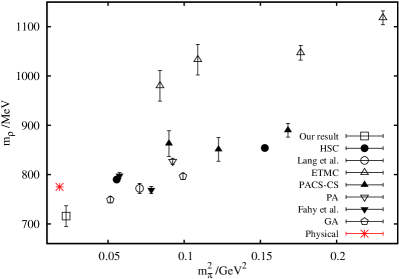
Figure 7: $\rho$ resonance masses from this (leftmost open square) and previous lattice calculations by the Hadron Spectrum Collaboration (HSC) Dudek et al. (2013); Wilson et al. (2015a), Lang et al. Lang et al. (2011), ETMC Feng et al. (2011), PACS-CS Aoki et al. (2007, 2011), Pelissier and Alexandru (PA) Pelissier and Alexandru (2013), Bulava et al. Bulava et al. (2015) and Guo and Alexandru (GA) Guo and Alexandru (2015). The physical value is also plotted Olive et al. (2014). Open symbols correspond to simulations with $N_{f}=2$ sea quark flavours, full symbols to $N_{f}=2+1$. In none of the cases was the continuum limit taken and no study includes systematic errors.

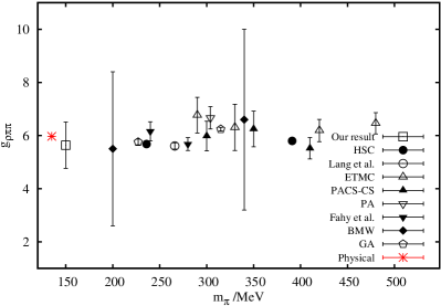
Figure 8: Breit-Wigner couplings from various lattice calculations (Hadron Spectrum Collaboration (HSC) Dudek et al. (2013); Wilson et al. (2015a), Lang et al. Lang et al. (2011), ETMC Feng et al. (2011), PACS-CS Aoki et al. (2007, 2011), Pelissier and Alexandru (PA) Pelissier and Alexandru (2013), Bulava et al. Bulava et al. (2015), BMW-c Frison et al. (2010) and Guo and Alexandru (GA) Guo and Alexandru (2015)) and that extracted from the experimentally measured $\rho$ meson width Olive et al. (2014). Open symbols correspond to $N_{f}=2$ results, full symbols to $N_{f}=2+1$.

In Fig. 8 we show the coupling $g_{\rho\pi\pi}$, obtained in Refs. Aoki et al. (2007); Feng et al. (2011); Frison et al. (2010); Lang et al. (2011); Aoki et al. (2011); Pelissier and Alexandru (2013); Dudek et al. (2013); Wilson et al. (2015a); Bulava et al. (2015); Guo and Alexandru (2015). Up to $m_{\pi}\approx 400\,\textmd{MeV}$, Ref. Peláez and Ríos (2010) expects the coupling $g_{\rho\pi\pi}$ to decrease (increase) by about 5% at NLO (NNLO), as a function of the pion mass, i.e., within the accuracy of their approach, $g_{\rho\pi\pi}$ is constant and the reduction of the decay width is purely due to phase space. An almost constant behaviour is also suggested by the Kawarabayashi-Suzuki-Riazuddin-Fayyazuddin relation Kawarabayashi and Suzuki (1966); Riazuddin and Fayyazuddin (1966), $g_{\rho\pi\pi}\approx m_{\rho}/f_{\pi}\approx 5.96$, where $f_{\pi}=\sqrt{2}F_{\pi}\approx 130\,\textmd{MeV}$ at the physical point. In Fig. 8, indeed, the lattice values for pion masses up to $m_{\pi}\approx 470\,\textmd{MeV}$ are all around this coupling (which is indistinguishable from the physical coupling $g_{\rho\pi\pi}\approx 5.93$, also shown in the figure). However, the noise increases significantly, closer to the physical pion mass, so $g_{\rho\pi\pi}$ can be extracted much more accurately at large quark masses. Again note that the lattice results were obtained at different lattice spacings with different actions and have quite different systematics.

For $K\pi$ scattering only a few previous lattice studies exist. At $m_{\pi}\approx 150\,\textmd{MeV}$ and at our lattice spacing, we find (Eqs. (25) and (19)) $m_{K^{*}}=868(13)(26)\,\textmd{MeV}$ and $g_{K^{*}\pi\pi}=4.79(49)$. Note that in experiment $m_{K^{*}}\approx 896\,\textmd{MeV}$ and $g_{K^{*}K\pi}\approx 5.39$. The Hadron Spectrum Collaboration Wilson et al. (2015b) reports $m_{K^{*}}=933(1)\,\textmd{MeV}$ and $g_{K^{*}K\pi}=5.72(52)$ at a pion mass of $391\,\textmd{MeV}$. Prelovsek et al. Prelovsek et al. (2013) use $m_{\pi}=266\,\textmd{MeV}$ and obtain $m_{K^{*}}=891(14)\,\textmd{MeV}$ and $g_{K^{*}K\pi}=5.7(1.6)$ while Fu and Fu Fu and Fu (2012) find $m_{K^{*}}=1014(27)\,\textmd{MeV}$ and $g_{K^{*}\pi\pi}=6.38(78)$, using a lattice spacing of $0.15\,\textmd{fm}$ and a pion mass of $240\,\textmd{MeV}$.

IV Conclusions

In summary, we have demonstrated the feasibility of computing resonance scattering parameters at a nearly physical pion mass. In particular, we computed the $p$-wave scattering phase shifts for $\pi\pi$ scattering in the $I=1$ channel and $K\pi$ in the $I=1/2$ channel. From these, we extracted the masses and couplings $m_{\rho}=716(21)(21)\,\textmd{MeV}$, $\Gamma_{\rho}=113(35)(3)\,\textmd{MeV}$, $m_{K^{*}}=868(13)(26)\,\textmd{MeV}$ and $\Gamma_{K^{*}}=30(6)(1)\,\textmd{MeV}$. The masses are lower than the experimental ones, $m_{\rho}\approx 775\,\textmd{MeV}$, $m_{K^{*}}\approx 896\,\textmd{MeV}$, and at least the width of the $K^{*}$ meson is underestimated too, in part due to a 10% heavier than physical pion. The values from experiment are: $\Gamma_{\rho}\approx 148\,\textmd{MeV}$, $\Gamma_{K^{*}}\approx 47\,\textmd{MeV}$ Olive et al. (2014). The second errors reflect an overall scale uncertainty of 3% Bali et al. (2013). While for the $\rho$ meson mass and width this error can be added in quadrature to the statistical one, for the $K^{*}$ parameters it is not straightforward to account for this uncertainty as our strange quark mass was tuned, assuming $a^{-1}=2.76\,\textmd{GeV}$. It is clear that we undershoot the experimental $\rho$ resonance mass by about two standard deviations, which indicates that not all systematics have been accounted for, in particular only one (albeit small) lattice spacing was realized. The corresponding positions of the resonance poles in the second Riemann sheet from analytical continuation are shown in Tables 3 and 4 and, at our present level of error, these cannot be distinguished from the above Breit-Wigner fit results.

The stochastic one-end source method we have used is cheaper compared to other methods Peardon et al. (2009); Morningstar et al. (2011); Fahy et al. (2015), as long as the set of kinematic points (and interpolators) is suitably restricted. In our calculation, we were able to recycle many propagators, by keeping one of the momenta, $\mathbf{p}_{1}$, fixed. The number of inversions required is given in Eq. (7) and the cost of including additional momenta is large. This is a limitation in particular for larger volumes, when the density of states increases and the use of multiple two-particle interpolators cannot be avoided. We remark, however, that our larger volume with a linear lattice extent $64a\approx 4.6\,\textmd{fm}$ is not at all small considering present-day standards in lattice scattering computations.

An alternative approach is the distillation method Peardon et al. (2009), which has been used in several other scattering calculations Dudek et al. (2013); Lang et al. (2011); Wilson et al. (2015a). This method does not suffer from a large computational overhead when including additional momenta as time-slice-to-all propagators (perambulators) are used in constructing the correlators. However, this method is not very well suited to large volumes as the number of vectors required increases in proportion to $L^{3}N_{t}$ and the cost of contractions also scales with a power of the number of vectors. Combining this method with stochastic estimates Morningstar et al. (2011) may ultimately not change this scaling behaviour but may make realistic lattice sizes accessible. Indeed, this stochastic distillation method has been successfully employed for $\pi\pi$ scattering Fahy et al. (2015); Bulava et al. (2015), where the number of solves used in Ref. Bulava et al. (2015) is not much higher than ours. It will be very interesting to see if such calculations can be pushed towards small quark masses, large volumes and time distances of about $1\,\textmd{fm}$ that allow for a reliable extraction of energy levels. Stochastic distillation was also successfully used to study $DK$ scattering Mohler et al. (2013); Lang et al. (2014, 2015).

Our calculation is performed at a single lattice spacing and it is not possible to quantify the size of discretization effects. For the action we use, these are of $\mathcal{O}(a^{2})$ and it is unlikely at our lattice spacing $a\approx 0.071\,\textmd{fm}$ that they are much larger than our 3% scale uncertainty. Limited information for the $\mathcal{O}(a^{2})$ accurate twisted mass action can be extracted from the results for the $\rho$ meson mass given in Ref. Burger et al. (2014). In this study of the hadronic vacuum polarization contribution to $(g-2)_{\mu}$, the correlators for vector mesons are calculated only using a one-particle interpolator for several ensembles with different lattice spacings and (larger than physical) pion masses. The mass of the $\rho$ is then found by treating it as a stable particle and the results obtained show no significant dependence on the lattice spacing. We therefore assume that the 3% scale uncertainty and the 10% larger than physical pion mass are dominant systematics but we cannot exclude other sources of error, in particular lattice spacing effects or the omission of the strange quark from the sea.

In Figs. 7 and 8 we compare our results on the $\rho$ meson mass and coupling to those of other lattice studies that were carried out at larger pion masses. The coupling $g_{\rho\pi\pi}$ appears to be remarkably independent of the quark mass and also robust against other systematics.

Future work will extend the present study to $N_{f}=2+1$ flavour configurations, including several lattice spacings, to enable a continuum limit extrapolation. Working close to the physical pion mass is particularly valuable for simulations of scattering processes involving states that are near to thresholds, e.g., $X(3872)$ and $D\overline{D}^{*}$ or $D_{s0}(2317)$ and $DK$, where the gap relative to the threshold strongly depends on the light quark mass.