Emergent universe in Hořava-Lifshitz-like $F(R)$ gravity

Abstract

We investigate the Einstein static universe (ESU) and the emergent universe scenario in the framework of Hořava-Lifshitz-like $F(R)$ gravity. We first perform a dynamical analysis in the phase space, and amongst others we show that a spatially open universe filled with matter satisfying the strong energy condition can exhibit a stable static phase. Additionally, we examine the behavior of the scenario under scalar perturbations and extract the conditions under which it is free of perturbative instabilities, showing that the obtained background ESU solutions are free of such instabilities. However, in order for the Einstein static universe to give rise to the emergent universe scenario we need to have an exotic matter sector that can lead the universe to depart from the stable static state and enter into its usual expanding thermal history.

I Introduction

According to the scenario of old Big-Bang cosmology based on the theory of general relativity (GR), our universe has begun from a finite past including an initial singularity, which is widely considered as a conceptual disadvantage. Furthermore, since standard Big-Bang cosmology was incapable of solving the horizon, flatness and magnetic monopole problems at early universe the inflation mechanism was introduced Inflation . Finally, in order to describe the late-time acceleration a small positive cosmological constant was added, giving rise to the Standard Model of the Universe, namely $\Lambda$CDM cosmology. However, despite the remarkable achievements of this paradigm, its physical content, concerning both early and late-time accelerating phases, is still ambiguous, and moreover amongst others one still faces the “initial singularity problem”.

Concerning the initial singularity problem, one could try to confront it through the “emergent universe” scenario Ellis . In particular, in such a scenario the universe is originated from a static state, known as “Einstein static universe” (ESU), and then it entered the inflationary phase, without ever passing through the Big-Bang singularity. However, remaining in the GR framework, and despite fine-tuning, perturbation analysis shows that the initial singularity cannot be completely removed. Indeed, ESU is severely influenced by the initial conditions such as perturbations which are prevailed in the Ultra-Violet (UV) limit, and it is indeed unstable against classical perturbations which eventually make it collapse towards a singularity Eddington .

In order to alleviate the above problems, alternative cosmological models have been developed. A first direction is to introduce new, exotic, forms of matter, which in the framework of general relativity could provide an explanation of the observed universe behavior Copeland:2006wr ; Cai:2009zp . A second direction is to modify the gravitational sector, obtaining a theory that still possess GR as a particular limit, but still being able to describe the universe at large scales through the extra gravitational degrees of freedom Nojiri:2006ri ; Capozziello:2011et . Indeed, in modified gravity, amongst others one can cure the emergent universe scenario, by making stable Einstein static universe. Hence, a large amount of activity was devoted to the study of the stability of the Einstein static universe in various gravitational modifications, such as Einstein-Cartan theory EC , Lyra geometry sadra , non-constant pressure models ncp , $f(R)$ gravity f(R) , $f(T)$ gravity f(T) , loop quantum cosmology LQC , massive gravity MG and doubly general relativity DGR , induced matter theory IMT , braneworld models brane , etc.

One interesting gravitational modification, proposed by Hořava, is the so-called Hořava-Lifshitz gravity Peter . This construction was motivated by the observation that the insertion of higher-order derivative terms in the Einstein-Hilbert Lagrangian establishes renormalizability, since the graviton propagator at high energies is modified Stelle:1976gc ; Biswas:2011ar . Nevertheless, this leads to a severe problem, since the equations of motion involve higher-order time derivatives and hence the theory includes ghosts. However, since it is the higher spatial derivatives that improve renormalizability while it is the higher time derivatives that lead to ghosts, one could think of constructing a theory that would allow for the inclusion of higher spatial derivatives only. Indeed, this is what it is achieved in Hořava-Lifshitz theory Peter , and since higher spatial derivatives are not accompanied by higher time ones, in the UV the theory exhibits power-counting renormalizability but still without ghosts. Such a theory definitely violates Lorentz invariance, however it presents GR as an Infra-Red fixed point, where Lorentz invariance is restored. Application of Hořava-Lifshitz gravity in a cosmological framework leads to very interesting behavior in agreement with observations Review . Finally, one can proceed further by construction extensions such as $F(R)$ Hořava-Lifshitz gravity Kluson1 , since in such scenarios one can obtain a unified mechanism for the early-time inflation and the late-time acceleration Chaichian1 .

From the above discussion we deduce that it is worthy to examine the realization of ESU and of the emergent universe scenario in the framework of Hořava-Lifshitz gravity and its extensions. The stability issues of the ESU in the framework of an IR modification of Hořava-Lifshitz gravity, representing a soft breaking of the so-called “detailed balance condition”, against linear homogeneous scalar perturbations, was explored in HL . As it is shown, there exists a large class of stable solutions, for large regions of barotropic equation-of-state parameter and model parameters, however the possibility for a transition to the inflationary era is ambiguous. Additionally, in the context of original Hořava-Lifshitz gravity such a study was performed in P , where it was shown that a stable ESU can be realized in the presence of a negative cosmological constant, however although the Big Bang singularity can be avoided the transition from this stable state to the inflationary era is impossible. On the other hand, in the case of the generalized version of Hořava-Lifshitz gravity T , it was shown that if the cosmic scale factor satisfies certain conditions initially and if the equation-of-state parameter approaches a critical value, the corresponding stable critical point coincides with the unstable one, and consequently a phase transition to the inflationary era can be provided P .

In the present work we are interested in studying the emergent universe scenario in the framework of a Hořava-Lifshitz-like $F(R)$ gravity, and in particular in investigating the realization and stability of the Einstein static universe and the possibility of the phase transition to the inflationary era. The plan of the manuscript is the following: In section II, we briefly review Hořava-Lifshitz-like $F(R)$ gravity and we apply it in a cosmological framework. In section III, we perform a dynamical analysis in the phase space, while in section IV, we extract the conditions under which the scenario at hand is stable against scalar perturbations. Finally, section V is devoted to discussion and conclusions.

II Hořava-Lifshitz-like $F(R)$ gravity and cosmology

In this section we review the $F(R)$ Hořava-Lifshitz theory Kluson1 (see also Chaichian1 ; Kluson2 ; Gourgoulhon ). In this construction one starts from the usual Hořava-Lifshitz gravity Peter and adds the $F(R)$ sector FR , namely one replaces the Ricci scalar $R$ by arbitrary functions of it.

We start by using the Arnowitt-Deser-Misner (ADM) formalism in a (3+1) space-time ADM , writing the metric as

$$ds^{2}=-N^{2}dt^{2}+h_{ij}(dx^{i}+N^{i}dt)(dx^{j}+N^{j}dt),$$ (1)

with $i,j=1,2,3$, where $N$, $N^{i}$ and $h_{ij}$ are respectively the lapse function, the shift function and the metric of three-dimensional spatial hypersurface $\Sigma_{t}$. In the framework of standard $F(R)$ gravity, the modified action is Chaichian1

$$S_{F(R)}=\int d^{4}x\,\sqrt{-g}\,\,F(R),$$ (2)

with $\sqrt{-g}=\sqrt{h}N$, where $F(R)$ denotes an arbitrary function of the scalar curvature $R$. This is given by

$$R=R^{(3)}+K^{ij}K_{ij}-K^{2}+2\nabla_{\mu}(n^{\mu}\nabla_{\nu}n^{\nu}-n^{\nu}\nabla_{\nu}n^{\mu})~{},$$ (3)

where $R^{(3)}$, $K_{ij}$ and $n^{\mu}$ are the three-dimensional scalar curvature, extrinsic curvature and a unit vector perpendicular to the three-dimensional spacelike hypersurface $\Sigma_{t}$, respectively. The term $R^{(3)}$ is an object associated with the spatial metric $h_{ij}$ of the hypersurface, and $K_{ij}$ is defined as

$$K_{ij}=\frac{1}{2N}(\dot{h_{ij}}-\nabla_{i}^{(3)}N_{j}-\nabla_{j}^{(3)}N_{i})~{}.$$ (4)

Hence, one can now write down the action of $F(R)$ Hořava-Lifshitz gravity as Chaichian1 ; Kluson2

$$S_{F(\tilde{R})}=\int dtd^{3}x\sqrt{h}\,N\,F(\tilde{R})~{},$$ (5)

with the extended scalar curvature $\tilde{R}$ given by

$$\tilde{R}\equiv K^{ij}K_{ij}-\lambda K^{2}+2\mu\nabla_{\mu}(n^{\mu}\nabla_{\nu}n^{\nu}-n^{\nu}\nabla_{\nu}n^{\mu})$$

$$\ \ \ \ \ \ -E^{ij}{\cal{G}}_{ijkl}E^{kl}~{}.$$ (6)

In the above expression the running dimensionless constant $\lambda$ appears due to the “super-metric”, defined on the hypersurface $\Sigma_{t}$ as

$${\cal{G}}^{ijkl}=\frac{1}{2}\left(h^{ik}h^{jl}+h^{il}h^{jk}\right)-\lambda h^{ij}h^{kl}~{},$$ (7)

while $E^{kl}$ has been inserted in order to embed the satisfaction of the “detailed balance condition”, which is defined by an action $W[h_{kl}]$ on $\Sigma_{t}$ as

$$\frac{\delta W[h_{kl}]}{\delta h_{ij}}=\sqrt{h}E^{ij}\;.$$ (8)

The detailed balance condition was inspired by the condensed matter physics cond and it implies that the potential term in the Lagrangian of a $D+1$ dimensional theory is derivable from the variation of the $D$ dimensional action Peter . In particular, while the shift variables $N^{i}(t,\textbf{x})$ and spatial metric $h_{ij}(t,\textbf{x})$ are function of both space and time, the lapse variable is assumed to be a function of time only, namely $N=N(t)$, an assumption compatible with the foliation preserving diffeomorphism.

In the initial formulation of $F(R)$ Hořava-Lifshitz gravity Kluson1 ; Kluson2 Kluson focused on a Lagrangian of a new class of $F(R)$ gravity theories with respect to the projectability condition, namely

$${\cal{L}}=N\sqrt{g}\bigg{[}\frac{2K_{ij}{\cal{G}}^{ijkl}K_{kl}}{F^{\,{}^{\prime}}(A)\kappa^{2}}-\kappa^{2}F(A)\bigg{]},$$ (9)

where $F(A)$ is an arbitrary function of the auxiliary field $A$, which is a function of $K_{ij}$ and $g_{ij}$, namely

$$A=\bigg{(}\frac{E^{ij}{\cal{G}}_{ijkl}E^{kl}+4\kappa^{-4}K_{ij}{\cal{G}}^{ijkl}K_{kl}}{1-4\kappa^{-4}K_{ij}{\cal{G}}^{ijkl}K_{kl}}\bigg{)}.$$ (10)

By setting the typical function $F(A)=\sqrt{1+A}-1$, the corresponding action $S=\int dtd^{3}x{\cal{L}}$ reads as

$$\!\!\!\!\!\!\!\!\!\!\!\!\!\!\!\!S=-\kappa^{2}\int dtd^{3}x\sqrt{h}N\left\{\sqrt{1+\frac{1}{4}E^{ij}{\cal{G}}_{ijkl}E^{kl}}\right.$$

$$\ \ \left.\cdot\sqrt{1-\frac{4}{\kappa^{4}}(K^{ij}K_{ij}-\lambda K^{2})}-1\right\}+S_{m},$$ (11)

with $\kappa^{2}\equiv 32G\pi c$ the gravitational constant, set for simplicity to $1$ in the following. In the above action we have also considered the matter sector characterized by $S_{m}$. Additionally, one could extend this action in a non-projectable version Kluson2 . We mention that the scenario of action (II) is invariant under the foliation preserving diffeomorphism and not under the full $D+1$ diffeomorphism, which is in contrast to the usual $F(R)$ gravity theories.

The linearized version of the action (II) writes as

$$\!\!\!\!\!\!\!\!\!\!\!\!\!\!\!\!S=\int dtd^{3}xN\sqrt{g}\left[\frac{2}{\kappa^{2}}(K_{ij}K^{ij}-\lambda K^{2})\right.$$

$$\ \ \ \ \ \ \ \ \ \ \ \ \left.-\frac{\kappa^{2}}{8}E^{ij}{\cal{G}}_{ijkl}E^{kl}\right],$$ (12)

which as expected reproduces the original Hořava-Lifshitz action. On the other hand, note that by choosing $\lambda=\mu=1$ in (II), one obtains the usual $F(R)$ gravity. Therefore, the non-linear action (II) is a form of Hořava-Lifshitz-like $F(R)$ gravity (see Kluson1 ; Chaichian1 ; Kluson2 ). More precisely, the Lagrangian density of the action (II) is not of the exact $F(R)$ form with any modified scalar curvature expression. Instead, it belongs to a class of models where the Lagrangian depends on the kinetic term $K_{ij}\mathcal{G}^{ijkl}K_{kl}$ and the potential term $E^{ij}\mathcal{G}_{ijkl}E^{kl}$ in a different way, and not only on the sum of the kinetic and the potential terms, as in the modified scalar curvature (II) (note that such more general modified Hořava-Lifshitz theories, where the Lagrangian can depend on the kinetic and potential terms independently, have also been considered in Chaichian1 ).

In order to apply the above theory in a cosmological framework, that is in order to construct Hořava-Lifshitz-like $F(R)$ cosmology, we impose an FRW metric on the 3-hypersurface $\Sigma_{t}$, namely

$$h_{ij}dx^{i}dx^{j}=a(t)^{2}\left[\frac{dr^{2}}{1-kr^{2}}+r^{2}(d\theta^{2}+\sin^{2}\theta d\varphi^{2})\right]~{},$$ (13)

where $a(t)$ is the scale factor and with $k=-1,\,0$ and $1$ corresponding to open, flat and closed universe, respectively. Furthermore, concerning the matter content of the universe, we consider it to be a perfect fluid with energy-momentum tensor in co-moving coordinates given by

$$T_{\mu\nu}=(\rho+p)u_{\mu}u_{\nu}+pg_{\mu\nu},$$ (14)

where $u_{\alpha}=\delta^{0}_{\alpha}$ is the four-velocity vector of the fluid, and $\rho$ and $p$ are the energy density and isotropic pressure, respectively. Under these assumptions, the field equations derived from action (II) give rise to the Friedmann equations, which write as Sayan :

$$\!\!\!H^{2}=\frac{1}{6(3\lambda-1)(1-\rho)^{2}}\left[\rho-\frac{1}{2}\rho^{2}+6\Lambda_{w}-\frac{12k}{a^{2}}+\frac{6k^{2}}{\Lambda_{w}a^{4}}\right],$$ (15)

$$\!\!\!\!\!\!\!\!\!\!\!\!\dot{H}=\frac{1}{4(3\lambda-1)(1-\rho)^{2}}\left[(\rho+p)(\rho-1)+\frac{8k}{a^{2}}+\frac{8k^{2}}{|\Lambda_{w}|a^{4}}\right]$$

$$\,-3(\rho+p)H^{2}(1-\rho)^{-1}.$$ (16)

The parameter $\Lambda_{\omega}$ is the effective cosmological constant, which similarly to the original version of Hořava-Lifshitz model must be negative for the running coupling parameter $\lambda>\frac{1}{3}$. We mention that the above equations include a negative energy density squared term $\rho^{2}$, which can have a significant role for the early stage of the universe. Technically speaking, the presence of $\rho^{2}$ term in the above Friedmann equations is a direct upshot of nonlinear dependence to matter source in this modified gravity theory in the early universe. A detailed discussion on this subject is presented in Sayan . Finally, let us point out that the value of $\lambda$ is commonly divided into two ranges, namely $0<\lambda<\frac{1}{3}$ and $\lambda>\frac{1}{3}$. However, phenomenological studies analyzing the observational data suggest that the value of $\lambda$ is constrained in a narrow range around $\lambda=1$, i.e. $|\lambda-1|\lesssim 0.02$ Dutta:2009jn , which was expected since GR is obtained for $\lambda=1$. Hence, in the following we restrict our analysis in the regime $\lambda>\frac{1}{3}$.

The cosmological application of Hořava-Lifshitz-like $F(R)$ gravity proves to have many interesting features Chaichian1 . Amongst others it can provide a unified mechanism for the description of both the early-time inflation and the late-time acceleration, or alternatively it can give rise to bouncing solutions Sayan that can cure the initial-singularity problem. Hence, it would be interesting to study if one can naturally obtain a stable Einstein static universe in such a theory. We mention that, as it is well-known, the versions of Hořava-Lifshitz gravity with the projectability condition suffer from the strong-coupling problem Bogdanos:2009uj . Although this can be alleviated by going beyond the projectability condition Blas:2009qj , the corresponding $F(R)$ extension would be too difficult to allow for an analytical investigation of the emergent universe scenario. Hence, in the present work we consider the Hořava-Lifshitz-like $F(R)$ gravity with the detailed balance and projectability condition as a first approach on the background cosmological evolution, having in mind that the investigation of the full theory is necessary as a next step.

III Dynamical analysis of Einstein static universe

In this section we intend to perform a phase-space analysis, investigating non-flat Hořava-Lifshitz-like $F(R)$ cosmology as a first-order cosmological dynamical system. This study will show whether the Einstein static universe (ESU) corresponds to a solution in which the universe can remain for very large time intervals. If this is not the case, then the realization of ESU will be highly improbable without a fine tuning of the initial conditions.

Using Taylor expansion in terms of $\frac{\rho}{\kappa^{2}}$ (note that we have set $\kappa^{2}=1$), the first and second Friedmann equations (15),(II) can be rewritten as

$$\!\!\!\!\!\!\!\!\!\!\!\!\!\!\!\!H^{2}=\frac{1}{6(3\lambda-1)}\left[\rho-\frac{5}{2}\rho^{2}+3\Lambda_{w}(\rho^{2}-\rho+1)\right.$$

$$\left.\!\!\!+6\left(\frac{k^{2}}{\Lambda_{w}a^{4}}-\frac{2k}{a^{2}}\right)(3\rho^{2}-2\rho+1)\right]+{\cal{O}}(\rho^{3}),\ \$$ (17)

and

$$\!\!\!\!\!\!\!\!\!\!\!\!\!\!\dot{H}=\frac{1}{4(3\lambda-1)}\Big{[}(\omega+1)\rho(3\rho-1)$$

$$\ \ \ \ \ \ \ \ \ \ \ \ \,\ +8\left(\frac{k}{a^{2}}+\frac{k^{2}}{|\Lambda_{w}|a^{4}}\right)(3\rho^{2}-2\rho+1)\Big{]}$$

$$\!-3(\omega+1)\rho(1+\rho)H^{2}+{\cal{O}}(\rho^{3})~{},$$ (18)

where we have neglected terms of the order $\rho^{3}$ and beyond. This means that only terms up to contribution of “dark radiations”, i.e $a^{-4}$, are kept. Also it is easy to check that in the leading order approximation, these reproduce the Friedmann equations in standard Hořava-Lifshitz gravity model. Additionally, in the above expressions we have considered the matter fluid to correspond to the standard barotropic one, with equation of state of the form $p=\omega\rho$.

Let us now focus on the ESU. This is described by $a=a_{0}$ and $\rho=\rho_{0}$, and hence the above Friedmann equations become

$$\!\!\!\!\!\!\!\!\!\!\!\!\!\!\!\!\!\frac{1}{6(3\lambda-1)}\left[\rho_{0}-\frac{5}{2}\rho_{0}^{2}+3\Lambda_{w}(\rho_{0}^{2}-\rho_{0}+1)\right.$$

$$\left.+6\left(\frac{k^{2}}{\Lambda_{w}a_{0}^{4}}-\frac{2k}{a_{0}^{2}}\right)(3\rho_{0}^{2}-2\rho_{0}+1)\right]=0,$$ (19)

$$\!\!\!\!\!\!\!\!\!\!\!\!\!\!\!\!\frac{1}{4(3\lambda-1)}\Big{[}(\omega+1)\rho_{0}(3\rho_{0}-1)$$

$$\!\!+8\left(\frac{k}{a_{0}^{2}}+\frac{k^{2}}{|\Lambda_{w}|a_{0}^{4}}\right)(3\rho_{0}^{2}-2\rho_{0}+1)\Big{]}=0.$$ (20)

For the case of spatially closed universe, i.e. for $k=+1$, equation (III) has two roots, namely

$$\left(\frac{1}{a_{0}^{2}}\right)_{1,2}=\frac{|\Lambda_{w}|}{2}\left(-1\pm\sqrt{1-\frac{g(\omega)}{|\Lambda_{w}|g_{0}}}\right),$$ (21)

with $g(\omega)$ and $g_{0}$ defined as

$$g(\omega)\equiv(3\rho_{0}^{2}-\rho_{0})\big{(}\omega+1\big{)}$$

$$g_{0}\equiv(6\rho_{0}^{2}-4\rho_{0}+2)~{}.$$ (22)

These two solutions correspond to two critical points. As we can straightforwardly see, for any barotropic parameter $\omega$ apart from $\omega=-1$, namely apart from a simple cosmological constant, both solutions (21) become unphysical since they lead to $\left(\frac{1}{a_{0}^{2}}\right)_{1,2}<0$. Similarly, for $\omega=-1$ the two critical points (21) become

$$\left(\frac{1}{a_{0}^{2}}\right)_{1}=0,\quad\quad\left(\frac{1}{a_{0}^{2}}\right)_{2}=-|\Lambda_{w}|~{},$$ (23)

which are both unphysical. Hence, none of these critical points signals the presence of an ESU in closed geometry, and thus they do not deserve further investigation.

For the case of open universe, i.e. for $k=-1$, equation (III) has two roots, namely

$$\left(\frac{1}{a_{0}^{2}}\right)_{1,2}=\frac{|\Lambda_{w}|}{2}\left(1\pm\sqrt{1-\frac{g(\omega)}{|\Lambda_{w}|g_{0}}}\right),$$ (24)

where

$$g(\omega)\equiv(3\rho_{0}^{2}-\rho_{0})\big{(}\omega+1\big{)}$$

$$g_{0}\equiv-(6\rho_{0}^{2}-4\rho_{0}+2)~{}.$$ (25)

Equation (24) will result in two real solutions provided that

$$3\bigg{[}(\omega+1)+2|\Lambda_{w}|\bigg{]}\rho_{0}^{2}$$

$$+\bigg{[}9(\omega+1)+4|\Lambda_{w}|\bigg{]}\rho_{0}+2|\Lambda_{w}|\geq 0~{}.$$ (26)

For the case $\omega=-1$ the above inequality holds for any value of $\rho_{0}>0$ and $|\Lambda_{w}|$, and thus we obtain two critical points, namely

$$\left(\frac{1}{a_{0}^{2}}\right)_{1}=0,\quad\quad\left(\frac{1}{a_{0}^{2}}\right)_{2}=|\Lambda_{w}|~{},$$ (27)

and thus only the latter is physical. By replacing it into (III) we obtain the corresponding energy density as

$$\!\!(\rho_{0})_{2}\!=\!\frac{39|\Lambda_{w}|-1}{104|\Lambda_{w}|-5}\left[1\pm\sqrt{1-\frac{(4788|\Lambda_{w}|-210)}{(1-39|\Lambda_{w}|)^{2}}}\right].$$ (28)

Both of them are physically acceptable (i.e. $(\rho_{0})_{2}>0$) with the condition

$$|\Lambda_{w}|>3~{},$$ (29)

however, and in order to be consistent with the expansion in terms of powers of $\rho$ in the background dynamic equations (III) and (III), we keep only the minus branch of (28). On the other hand, for $\omega<-1$ and $\omega>-1$, by requiring the physical condition $\rho_{0}>0$, we obtain the following bounds on the value of $|\Lambda_{w}|$, namely

$$-\frac{\omega+1}{2}<|\Lambda_{w}|<-(\omega+1)~{},$$ (30)

and

$$0<|\Lambda_{w}|<\frac{5(\omega+1)}{2}~{},$$ (31)

respectively, along with the common lower bound on the value of $\rho_{0}$:

$$\!\!\!\!\!\!\!\!\!\!\!\!\!\!\!\!\!\!\!\rho_{0}\geq\frac{1}{6(2|\Lambda_{w}|+\omega+1)}\left\{-9(\omega+1)+4|\Lambda_{w}|\right.$$

$$\!\!\!\!\!\!\!\!\left.+\sqrt{81(\omega+1)^{2}+48|\Lambda_{w}|(\omega+1)-32|\Lambda_{w}|^{2}}\right\}\!.$$ (32)

Hence, in summary, both solutions of (24) are physical when the constraints (30)-(III) are fulfilled. Finally, by inserting the solutions (24) into equation (III) we acquire

$$\!\!\!\!\!\!\!\!\!\!\!\!\!\left(30|\Lambda_{w}|+3\omega+\frac{1}{2}\right)\rho_{0}^{2}-\bigg{(}21|\Lambda_{w}|+\omega\bigg{)}\rho_{0}$$

$$+12|\Lambda_{w}|\pm\frac{9}{2}\sqrt{|\Lambda_{w}|^{2}g_{0}^{2}-|\Lambda_{w}|g_{0}g(\omega)}=0,$$ (33)

the solution of which will provide the corresponding $\rho_{0}$ for each solution. Since analytical solutions are impossible, we solve (III) numerically and in Table 1 we present the real and positive results for some representative values of $\Lambda_{w}$. Note that we focus on the negative-sign branch, since only this branch is consistent with $-1<\omega\leq 1/3$. Hence, we deduce that from the two static solutions in (24), only the positive-branch is compatible with $-1<\omega\leq 1/3$, namely

$$\left(\frac{1}{a_{0}^{2}}\right)_{2}=\frac{|\Lambda_{w}|}{2}\left(1+\sqrt{1-\frac{g(\omega)}{|\Lambda_{w}|g_{0}}}\right).$$ (34)

	$|\Lambda_{w}|=\frac{1}{40}$	$|\Lambda_{w}|=\frac{1}{60}$	$|\Lambda_{w}|=\frac{1}{80}$	$|\Lambda_{w}|=\frac{1}{100}$
$\omega=-2/3$	$0.423$	$0.413$	$0.407$	$0.404$
$\omega=0\ \$	$0.407$	$0.403$	$0.402$	$0.404$
$\omega=1/3$	$0.404$	$0.403$	$0.408$	$0.417$

Table 1: The physical values of $\rho_{0}$ arising numerically from (III), for the negative-sign branch, for various values of $\omega$ and $\Lambda_{w}$.

In order to study the stability of this critical point, inspired by the first-order dynamical system approach EllisDynamical ; Copeland:1997et , we consider the following two auxiliary variables

$$y_{1}=a,\quad\quad y_{2}=\dot{a},$$ (35)

which obey the following equations:

$$\!\!\!\!\!\!\!\!\!\!\!\!\!\!\!\dot{y_{1}}=y_{2}=f_{1}(y_{1},y_{2}),$$ (36)

$$\!\!\!\!\!\!\!\!\!\!\!\!\!\!\!\dot{y_{2}}=\frac{1}{4(3\lambda-1)}\Big{\{}(\omega+1)\rho(3\rho-1)y_{1}$$

$$\ \ \ \ \ \ \ \ \ +8\left(3\rho^{2}-2\rho+1\right)\Big{(}\frac{k}{y_{1}}+\frac{k^{2}}{y_{1}^{3}|\Lambda_{w}|}\Big{)}\Big{\}}$$

$$\!\!\!+\Big{[}1-3(\omega+1)\rho(\rho+1)\Big{]}\frac{y_{2}^{2}}{y_{1}}=f_{2}(y_{1},y_{2}).$$ (37)

As usual, by deriving the eigenvalues square $\vartheta^{2}$ of the Jacobian matrix

$$J\bigg{(}f_{1}(y_{1},y_{2}),f_{2}(y_{1},y_{2})\bigg{)}=\left(\begin{array}[]{cc}\frac{\partial f_{1}}{\partial y_{1}}&\frac{\partial f_{1}}{\partial y_{2}}\\ \frac{\partial f_{2}}{\partial y_{1}}&\frac{\partial f_{2}}{\partial y_{2}}\\ \end{array}\right),$$ (40)

one can deduce on the stability of the critical points. If $\vartheta^{2}<0$ then the corresponding critical point can be interpreted as a stable center point. Since, as it was mentioned above, for the closed universe there is not a physically accepted static solution, in the following we focus on the open case.

In the case of $\omega=-1$, after a simple calculation we acquire:

$$\!\!\!\!\!\!\!\!\!\!\mbox{Critical point }\left(\frac{1}{a_{0}^{2}}\right)_{2}=|\Lambda_{w}|,$$

$$\!\!\!\!\!\!\!\!\!\!\Longrightarrow\ \vartheta^{2}=\big{(}-12\rho_{0}^{2}+8\rho_{0}-4\big{)}\frac{|\Lambda_{w}|}{(3\lambda-1)},$$ (41)

and thus it implies the stability of ESU corresponding to the physical critical point $(y_{1},0)$, since $\vartheta^{2}|_{(\rho_{0})_{2}}<0$. In order to see this feature more transparently, in the upper graph of Fig. 1 we depict the phase-space behavior for the open geometry for $\omega=-1$. Additionally, in order to verify the stability of the ESU in an alternative way, we add a small deviation to the scale-factor value $(\frac{1}{a_{0}^{2}})_{2}=|\Lambda_{w}|$ and in the lower graph of Fig. 1 we depict its evolution, as it arises numerically from (36). As we observe the universe exhibits small oscillations around the scale-factor value of the ESU, without deviating from it, as expected.

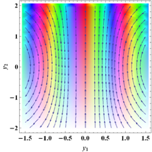
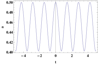
Figure 1: The phase diagram in $(a,\dot{a})$ or $(y_{1},y_{2})$ space (upper graph) and the evolution of the scale factor in terms of time (lower graph) for the spatially open cosmology, with equation-of-state parameter $\omega=-1$. We have set $\lambda=1$ and $|\Lambda_{w}|=5$, while for $\rho_{0}$ we have used the values obtained numerically from the negative-sign branch of (28), namely $\rho_{0}=0.148$.

In the case of $\omega\neq-1$, we acquire:

$$\vartheta^{2}=\frac{1}{4(3\lambda-1)}\left[(\omega+1)(3\rho_{0}^{2}-\rho_{0})\right.$$

$$\left.+8\bigg{(}3\rho_{0}^{2}-2\rho_{0}+2\bigg{)}\left(\frac{1}{a_{0}^{2}}-\frac{3}{|\Lambda_{w}|a_{0}^{4}}\right)\right],$$ (42)

with $a_{0}$ given in (34) and $\rho_{0}$ arising from (III), i.e from Table 1. In Table 2 we provide the corresponding values of $\vartheta^{2}$. As we observe, $\vartheta^{2}<0$ for all values of $|\Lambda_{w}|$,$\omega$ and ($a_{0},\rho_{0}$) consistent with $0\leq\rho_{0}<1$ and $-1<\omega\leq 1/3$, and thus we deduce that the ESU is stable.

	$|\Lambda_{w}|=\frac{1}{40}$	$|\Lambda_{w}|=\frac{1}{60}$	$|\Lambda_{w}|=\frac{1}{80}$	$|\Lambda_{w}|=\frac{1}{100}$
$\omega=-\frac{2}{3}$	$\vartheta^{2}=-0.37$	$\vartheta^{2}=-0.32$	$\vartheta^{2}=-0.3$	$\vartheta^{2}-0.28$
$\omega=0$	$\vartheta^{2}=-0.86$	$\vartheta^{2}=-0.82$	$\vartheta^{2}=-0.78$	$\vartheta^{2}=-0.76$
$\omega=\frac{1}{3}$	$\vartheta^{2}=-1.1$	$\vartheta^{2}=-1.06$	$\vartheta^{2}=-1.01$	$\vartheta^{2}=-0.98$

Table 2: The eigenvalues corresponding to the ESU critical points ($a_{0},\rho_{0}$) obtained from (34) and the values of $\rho_{0}$ given in Table 1, for $\lambda=1$.

However, although a stable ESU is easily realized, in order to obtain a full realization of the emergent universe scenario we need an additional mechanism that could make the universe deviate from ESU after a large time interval, and enter into the usual expanding thermal history. This would be possible only in the presence of an exotic matter sector, with equation-of-state parameter outside the range $-1<\omega\leq 1/3$.

IV Scalar perturbations and stability conditions

In this section we perform an analysis of the scalar perturbations in Hořava-Lifshitz-like $F(R)$ gravity in a cosmological framework. In particular, we desire to extract conditions under which the scenario at hand is free of perturbative instabilities, and hence physical. In order to achieve this, we linearly perturb equations (III) and (III) around the static states (III) and (III). Applying the following perturbations in the scale factor and matter density:

$$a(t)\rightarrow a_{0}(1+\delta a(t)),$$

$$\rho(t)\rightarrow\rho_{0}(1+\delta\rho(t))~{},$$ (43)

linearizing using

$$(1+\delta a(t))^{n}\simeq 1+n\delta a(t),$$

$$(1+\delta\rho(t))^{n}\simeq 1+n\delta\rho(t),$$ (44)

and imposing the background Friedmann equation (III) in order to eliminate background quantities, we obtain

$$\!\!\!\!\!\!\!\!\!\!\!\!\!\rho_{0}\delta\rho(t)\Big{\{}1-5\rho_{0}+6\Lambda_{w}(\rho_{0}-1)$$

$$\ \ \ \ \ +12\Big{(}\frac{2k}{a_{0}^{2}}-\frac{k^{2}}{\Lambda_{w}a_{0}^{4}}\Big{)}(1-3\rho_{0})\Big{\}}=$$

$$\!\!\!\!\!\!\!\!\!\!\!\!\!-\delta a(t)\Big{\{}24\Big{(}\frac{k}{a_{0}^{2}}-\frac{k^{2}}{\Lambda_{w}a_{0}^{4}}\Big{)}(1-2\rho_{0}+3\rho_{0}^{2})\Big{\}}.$$ (45)

Similarly, perturbing equation (III), linearizing, and imposing (III) in order to eliminate background quantities, we acquire

$$\!\!\!\!\!\!\!\!\!\!\delta\ddot{a}=\frac{1}{4(3\lambda-1)}\Big{\{}\rho_{0}\delta\rho\Big{[}(\omega+1)(2\rho_{0}-1)$$

$$\ \ \ +\frac{8k}{a_{0}^{2}}\rho_{0}(1+\omega)-16\Big{(}\frac{k}{a_{0}^{2}}+\frac{k^{2}}{|\Lambda_{w}|a_{0}^{4}}\Big{)}(1-3\rho_{0})\Big{]}$$

$$\ -\delta a\Big{[}16\Big{(}\frac{k}{a_{0}^{2}}+\frac{2k^{2}}{|\Lambda_{w}|a_{0}^{2}}\Big{)}(1-2\rho_{0}+3\rho_{0}^{2})\Big{]}\Big{\}}\;.$$ (46)

Thus, using (IV) in order to find $\rho_{0}\delta\rho$ in terms of $\delta a$, and substituting into (IV), leads to the following differential equation:

$$\delta\ddot{a}-\frac{\left(A\times B\times C-D\right)}{(3\lambda-1)}\delta a=0\;,$$ (47)

where we have defined

$$\!\!\!\!\!\!\!\!\!\!\!\!A\equiv-(6\rho_{0}\Lambda_{\omega}+\rho_{0}+1)+\frac{24k}{a_{0}^{2}}(1+3\rho_{0}^{2})$$

$$-\frac{12k^{2}}{\Lambda_{w}a_{0}^{4}}(1-3\rho_{0})+36\left(\Lambda_{\omega}-\frac{4k}{a_{0}^{2}}+\frac{2k^{2}}{\Lambda_{w}a_{0}^{4}}\right)^{2}$$

$$+\left(5-6\Lambda_{\omega}+\frac{72k}{a_{0}^{2}}-\frac{36k^{2}}{a_{0}^{2}}\right)\rho_{0}$$

$$\ \ \ \cdot\left(\rho_{0}-12\Lambda_{\omega}+\frac{48k}{a_{0}^{2}}-\frac{24k^{2}}{\Lambda_{w}a_{0}^{4}}\right),$$ (48)

$$B\equiv 2\left(\frac{k}{a_{0}^{2}}-\frac{k^{2}}{|\Lambda_{w}|a_{0}^{4}}\right)(1-2\rho_{0}+3\rho_{0}^{2}),$$ (49)

$$C\equiv 3(1+\omega)(2\rho_{0}-1)-48\left(\frac{k}{a_{0}^{2}}+\frac{k^{2}}{|\Lambda_{w}|a_{0}^{4}}\right)(1-3\rho_{0}),$$ (50)

and

$$D \equiv -4\left(\frac{k}{a_{0}^{2}}+\frac{2k^{2}}{|\Lambda_{w}|a_{0}^{4}}\right)(1-2\rho_{0}+3\rho_{0}^{2}).$$ (51)

Hence, from the differential equation (47) we deduce that in order to have a stable ESU against scalar perturbations in the framework of Hořava-Lifshitz-like $F(R)$ gravity, the following condition must be satisfied:

$$\frac{\left(A\times B\times C-D\right)}{3\lambda-1}<0\;.$$ (52)

As usual, the instabilities-absence condition (52) must be applied in the background solutions of the model, extracted in the previous section. Since we are dealing with Einstein static universe, these solutions were characterized only by $a_{0},\rho_{0},k$, with $\omega$ and $\Lambda_{w}$ the model parameters, and were summarized in expressions (27), (28), (34) and Table 1. Since in the case of a closed universe ESU was not realized, we focus on the case of open geometry. For the case $\omega=-1$, by setting the background configuration $(a_{0},\rho_{0})$ from equations (27) and (28), subject to the constraint (29), and substituting them into equations (IV)-(51), we immediately find that inequality (52) holds. Similarly, in the case $\omega\neq-1$, substituting the values of $a_{0}$ and $\rho_{0}$ from (34) and Table I into (IV)-(51) we deduce that inequality (52) is satisfied too. Hence, in summary, we can see that the ESU obtained in the precious section is free of perturbative instabilities.

V Remarks and Conclusions

In this work we performed an investigation of the Einstein static universe (ESU) in the framework of Hořava-Lifshitz-like $F(R)$ gravity. Such a gravitational modification is obtained by employing higher-order $R$-terms, keeping both the detailed balance and projectability conditions, and although contrary to the usual $F(R)$ gravity it is not full $D+1$ diffeomorphism invariant, in the limit of linear approximation it recovers the usual Hořava-Lifshitz counterpart. Hence, we were interested in examining whether the cosmological application of this theory allows for the realization of ESU, which is the basic concept in the realization of the emergent universe scenario. If this is the case, then the initial-singularity problem of standard Big-Bag cosmology can be alleviated.

As a first step we performed a dynamical analysis of Hořava-Lifshitz-like $F(R)$ cosmology in the phase space. We showed that in the case of closed geometry there is no stable physically meaningful ESU, while in the case of open geometry the ESU can be an attractor in the presence of both exotic and usual matter. However, the most physically interesting result was that in the case of open geometry ESU is stable and thus it can be realized. Nevertheless, in order to obtain a full realization of the emergent universe scenario we need an additional mechanism that could make the universe deviate from ESU after a large time interval, and enter into the usual expanding thermal history, which can be obtained only through an exotic matter sector with unconventional equation-of-state parameter.

As a second step we examined the behavior of ESU under scalar perturbations, desiring to extract the conditions under which the scenario at hand is free of perturbative instabilities such as ghosts or Laplacian instabilities. Our analysis showed that the background ESU solutions are free of perturbative instabilities.

The above results imply that ESU can be safely realized in the framework of Hořava-Lifshitz-like $F(R)$ cosmology, however the emergent universe scenario is not straightforward in such a gravitational modification, since an exotic form of matter is required. Hence, within the same theory we have both a cosmological advantage, namely that we alleviate the initial-singularity problem, as well as a theoretical advantage, namely that the underlying theory has an improved renormalizable behavior in the UV. These features make the above construction a good candidate for the description of Nature, that is worthy to be investigated further.

References

- (1) A. H. Guth, Phys. Rev. D 23, 347 (1981); K. Sato, Mon. Not. Roy. Astron. Soc. 195, 467 (1981); A. D. Linde, Phys. Lett. B 108, 389 (1982).
- (2) G. F. R. Ellis and R. Maartens, Class. Quant. Grav. 21, 223 (2004); G. F. R. Ellis, J. Murugan, and C. G. Tsagas, Class. Quant. Grav. 21, 233 (2004).
- (3) A. S. Eddington, Mon. Not. Roy. Astron. Soc. 90, 668 (1930); G. W. Gibbons, Nucl. Phys. B 310, 636 (1988); J. D. Barrow, G. F. R. Ellis, R. Maartens and C. G. Tsagas, Class. Quant. Grav. 20, L155 (2003).
- (4) E. J. Copeland, M. Sami and S. Tsujikawa, Int. J. Mod. Phys. D 15, 1753 (2006).
- (5) Y. F. Cai, E. N. Saridakis, M. R. Setare and J. Q. Xia, Phys. Rept. 493, 1 (2010).
- (6) S. Nojiri and S. D. Odintsov, eConf C0602061, 06 (2006), Int. J. Geom. Meth. Mod. Phys. 4, 115 (2007).
- (7) S. Capozziello and M. De Laurentis, Phys. Rept. 509, 167 (2011).
- (8) C. G. Bohmer, Class. Quant. Grav. 21, 1119 (2004); K. Atazadeh, JCAP 06, 020 (2014).
- (9) F. Darabi, Y. Heydarzade and F. Hajkarim, Canadian. J. Phys 93 (12), 1566 2015.
- (10) A. Ibrahim and Y. Nutku, Gen. Rel. Grav. 7, 949 (1976); C. G. Bohmer, Gen. Rel. Grav. 36, 1039 (2004); C. G. Bohmer and G. Fodor, Phys. Rev. D 77, 064008 (2008); K. Lake, Phys. Rev. D 77, 127502 (2008).
- (11) J. D. Barrow and A. C. Ottewill, J. Phys. A 16, 2757 (1983); C. G. Bohmer, L. Hollenstein and F. S. N. Lobo, Phys. Rev. D 76, 084005 (2007); R. Goswami, N. Goheer and P. K. S. Dunsby, Phys. Rev. D 78, 044011 (2008); N. Goheer, R. Goswami, and P. K. S. Dunsby, Class. Quant. Grav. 26, 105003 (2009); S. S. Seahra and C. G. Bohmer, Phys. Rev. D 79, 064009 (2009).
- (12) P. Wu, H. Yu, Phys. Lett. B 703, 223 (2011); J. T. Li, C. C. Lee, C. Q. Geng, Eur. Phys. J. C 73, 2315 (2013).
- (13) D. J. Mulryne, R. Tavakol, J. E. Lidsey and G. F. R. Ellis, Phys. Rev. D 71, 123512 (2005); L. Parisi, M. Bruni, R. Maartens and K. Vandersloot, Class. Quant. Grav. 24, 6243 (2007); R. Canonico and L. Parisi, Phys. Rev. D 82, 064005 (2010).
- (14) L. Parisi, N. Radicella and G. Vilasi, Phys.Rev. D 86, 024035 (2012); L. Parisi, N. Radicella and G. Vilasi, Springer Proc. Math. Stat 60, 355 (2014); K. Zhang, P. Wu, H. Yu, Phys.Rev. D 87, 063513 (2013).
- (15) M. Khodadi, Y. Heydarzade, K. Nozari and F. Darabi, Eur. Phys. J. C 75, 590 (2015).
- (16) Y. Heydarzade, F. Darabi, JCAP 04, 028 (2015).
- (17) L. Gergely, R. Maartens, Class. Quant. Grav. 19, 213 (2002); K. Zhang, P. Wu, H. Yu, Phys. Lett. B 690 229 (2010); K. Zhang, P. Wu, H. Yu, Phys. Rev. D 85, 043521 (2012); C. Clarkson, S. S. Seahra, Class. Quant. Grav. 22 3653 (2005); K. Atazadeh, Y. Heydarzade and F. Darabi, Phys. Lett. B 732, 223 (2014); Y. Heydarzade, F. Darabi, K. Atazadeh, arXiv:1511.03217.
- (18) P. Hor̂ava, Phys. Rev. D 79, 084008 (2009); P. Hor̂ava, JHEP 0903, 020 (2009); P. Hor̂ava, Phys. Rev. Lett. 102, 161301 (2009).
- (19) K. S. Stelle, Phys. Rev. D 16, 953 (1977).
- (20) T. Biswas, E. Gerwick, T. Koivisto and A. Mazumdar, Phys. Rev. Lett. 108, 031101 (2012).
- (21) E. Kiritsis and G. Kofinas, Nucl. Phys. B 821, 467 (2009); G. Calcagni, Phys. Rev. D 81, 044006 (2010); E. N. Saridakis, Eur. Phys. J. C 67, 229 (2010); D. Orlando and S. Reffert, Class. Quant. Grav. 26, 155021 (2009); S. Mukohyama, Phys. Rev. D 80, 064005 (2009); Y. S. Piao, Phys. Lett. B 681, 1 (2009); M. i. Park, JHEP 0909, 123 (2009); S. Mukohyama, JCAP 0906, 001 (2009); R. G. Cai, L. M. Cao and N. Ohta, Phys. Lett. B 679, 504 (2009); G. Leon and E. N. Saridakis, JCAP 0911, 006 (2009); H. Lu, J. Mei and C. N. Pope, Phys. Rev. Lett. 103, 091301 (2009); S. R. Das and G. Murthy, Phys. Rev. D 80, 065006 (2009); J. Kluson, Phys. Rev. D 80, 046004 (2009); A. Ali, S. Dutta, E. N. Saridakis and A. A. Sen, Gen. Rel. Grav. 44, 657 (2012); A. Wang and R. Maartens, Phys. Rev. D 81, 024009 (2010); J. J. Peng and S. Q. Wu, Eur. Phys. J. C 66, 325 (2010); A. Ghodsi and E. Hatefi, Phys. Rev. D 81, 044016 (2010); S. Nojiri and S. D. Odintsov, Phys. Rev. D 81, 043001 (2010); Y. S. Myung, Phys. Rev. D 81, 064006 (2010); X. Gao, Y. Wang, R. Brandenberger and A. Riotto, Phys. Rev. D 81, 083508 (2010); E. N. Saridakis, Gen. Rel. Grav. 45, 387 (2013); F. Kheyri, M. Khodadi, H. R. Sepangi, Eur. Phys. J. C 73, 2286 (2013); M. Khodadi, H. R. Sepangi, Annals Phys. 346, 129 (2014); D. W. Pang, Commun. Theor. Phys. 62, 265 (2014).
- (22) J. Kluson, JHEP 0911, 078 (2009).
- (23) M. Chaichian, S. Nojiri, S. D. Odintsov, M. Oksanen, and A. Tureanu, Class. Quantum Grav. 27, 185021 (2010); S. Carloni, M. Chaichian, S. Nojiri, S. D. Odintsov, M. Oksanen and A. Tureanu, Phys. Rev. D 82, 065020 (2010).
- (24) C. G. Bohmer and F. S. N. Lobo, Eur. Phys. J. C 70, 1111 (2010).
- (25) P. Wu and H. W. Yu, Phys. Rev. D 81, 103522 (2010).
- (26) T. P. Sotiriou, M. Visser, and S. Weinfurtner, Phys. Rev. Lett. 102, 251601 (2009); T. P. Sotiriou, M. Visser, and S. Weinfurtner, JHEP 0910, 033 (2009).
- (27) J. Kluson, Phys. Rev. D 81, 064028 (2010).
- (28) E. Gourgoulhon, gr-qc/0703035.
- (29) S. Nojiri and S. D. Odintsov, Int. J. Geom. Meth. Mod. Phys. 4, 115 (2007); A. De Felice, S. Tsujikawa, Living Rev. Rel. 13, 3 (2010).
- (30) R. L. Arnowitt, S. Deser and C. W. Misner, Gen. Rel. Grav. 40, 1997 (2008).
- (31) E. Ardonne, P. Fendley and E. Fradkin, Annals Phys. 310, 493 (2004).
- (32) K. Sayan, Chakrabarti, Koushik Dutta, Anjan A. Sen, Phys. Lett. B 711, 147 (2012).
- (33) S. Dutta and E. N. Saridakis, JCAP 1001, 013 (2010); S. Dutta and E. N. Saridakis, JCAP 1005, 013 (2010).
- (34) C. Bogdanos and E. N. Saridakis, Class. Quant. Grav. 27, 075005 (2010).
- (35) D. Blas, O. Pujolas and S. Sibiryakov, Phys. Rev. Lett. 104, 181302 (2010).
- (36) Dynamical Systems in Cosmology, edited by J. Wainwright and G. F. R. Ellis, Cambridge University Press, Cambridge (1997).
- (37) E. J. Copeland, A. R. Liddle and D. Wands, Phys. Rev. D 57, 4686 (1998); P. G. Ferreira and M. Joyce, Phys. Rev. Lett. 79, 4740 (1997); X. m. Chen, Y. g. Gong and E. N. Saridakis, JCAP 0904, 001 (2009); G. Leon and E. N. Saridakis, JCAP 1303, 025 (2013).