Fermi polaron in a one-dimensional quasi-periodic optical lattice: the simplest many-body localization challenge

Abstract

We theoretically investigate the behavior of a moving impurity immersed in a sea of fermionic atoms that are confined in a quasi-periodic (bichromatic) optical lattice, within a standard variational approach. We consider both repulsive and attractive contact interactions for such a simplest many-body localization problem of Fermi polarons. The variational approach enables us to access relatively large systems and therefore may be used to understand many-body localization in the thermodynamic limit. The energy and wave-function of the polaron states are found to be strongly affected by the quasi-random lattice potential and their experimental measurements (i.e., via radio-frequency spectroscopy or quantum gas microscope) therefore provide a sensitive way to underpin the localization transition. We determine a phase diagram by calculating two critical quasi-random disorder strengths, which correspond to the onset of the localization of the ground-state polaron state and the many-body localization of all polaron states, respectively. Our predicted phase diagram could be straightforwardly examined in current cold-atom experiments.

I Introduction

Anderson localization of interacting disordered systems - a phenomenon referred to as many-body localization (MBL) - has received intense attention over the past few years Nandkishore2015 ; Altman2015 . Earlier studies focus on condensed matter systems, where a uniformly distributed white-noise disorder potential is often adopted to carry out perturbative analyses in the presence of weak interactions Basko2006 ; Aleiner2010 or numerical simulations with strong interactions Oganesyan2007 ; Pal2010 ; Bardarson2012 ; Mondaini2015 . Recent experimental advances in ultracold atoms provide a new paradigm to explore MBL Schreiber2015 ; Bordia2015 . In these experiments, a quasi-periodic bichromatic optical lattice has been used, leading to a quasi-random disorder potential Harper1955 ; Aubry1980 . The interatomic interaction and dimensionality of the system can be tuned at will, with unprecedented accuracy Bloch2008 .

It is well-known that Anderson localization occurs not only in the ground state of the system but also in highly excited states Evers2008 . In the presence of interactions, this fundamental feature makes both theoretical and experimental investigations of MBL extremely challenging Nandkishore2015 ; Altman2015 . To understand the localization of highly excited states, most theoretical studies of interacting disorder systems rely on the full exact diagonalization of the model Hamiltonian and therefore the size of the system is severely restricted Oganesyan2007 ; Pal2010 ; Mondaini2015 . On the other hand, in the recent two cold-atom experiments, only the localization of a particular type of (excited) states, i.e., a charge density wave state, has been examined Schreiber2015 ; Bordia2015 .

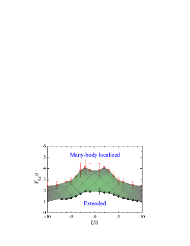
Figure 1: (Color online) Phase diagram of a fermionic polaron in quasi-random lattice potentials. The full circles with solid line show the threshold of entering a localized state for the ground-state polaron. The empty squares with dashed line give the critical disorder strength, above which all polaron states become localized. The error bars indicate the estimated uncertainty. The system has an unpure many-body energy spectrum in the shaded area, i.e., extended polaron states can coexist with localized polaron states. The average filling factor of fermionic atoms is $\left\langle\hat{n}\right\rangle=1/2$.

In this work, motivated by those rapid experimental advances, we propose to experimentally explore (arguably) the simplest case of MBL: a moving impurity immersed in a sea of non-interacting fermionic atoms. The latter is subjected to a one-dimensional (1D) quasi-periodic optical lattice Harper1955 and experiences Anderson localization when the disorder strength is sufficiently strong Aubry1980 . There is a contact interaction between impurity and fermionic atoms. The motion of impurity - or more precisely a Fermi polaron Chevy2006 ; Lobo2006 ; Achirotzek2009 ; Wenz2013 ; Massignan2014 - is therefore affected by the localization properties of fermionic atoms. The proposed system has several advantages to address the MBL phenomenon. Experimentally, it seems easier to measure a Fermi polaron. Its energy might be determined by using radio-frequency spectroscopy Achirotzek2009 while its wave-function might be identified from the in situ density profile through the recently developed quantum gas microscope for fermionic atoms Cheuk2015 ; Parsons2015 ; Omran2015 . Theoretically, we have well-controlled approximations to handle the Fermi polaron problem Chevy2006 , even in the limit of very strong interactions Lobo2006 ; Doggen2014 , which make it feasible to access large systems as those experimentally explored. Therefore, we may underpin a phase diagram of MBL in the thermodynamic limit.

Our main result is briefly summarized in Fig. 1. We determine two critical quasi-random disorder strengths within a variational approach, by taking into account the dominant single particle-hole excitation above the Fermi sea Chevy2006 . The first critical field (circles with solid line) corresponds to the onset of the Anderson localization of the ground-state polaron state. While at the second critical field (empty squares with dashed line), all polaron states become localized. This gives rise to a complete MBL phase diagram of Fermi polarons. It is amazing that even the interaction experienced by a single impurity can dramatically lead to the appearance of MBL. Our predicted phase diagram could be easily examined in current cold-atom experiments Schreiber2015 ; Bordia2015 .

II Model Hamiltonian and variational approach

A moving Fermi polaron in a 1D quasi-disordered lattice of length $L$ can be described by the model Hamiltonian Schreiber2015 ; Bordia2015 ,

$${\cal H} = \sum_{n=0}^{L-1}\left[\left(-t_{c}\hat{c}_{n}^{\dagger}\hat{c}_{n+1}+\text{H.c.}\right)+\left(-t_{d}\hat{d}_{n}^{\dagger}\hat{d}_{n+1}+\text{H.c.}\right)\right.$$ (1)

$$+\left.U\hat{c}_{n}^{\dagger}\hat{c}_{n}\hat{d}_{n}^{\dagger}\hat{d}_{n}+V_{0}\cos\left(2\pi n\beta+\theta\right)\hat{c}_{n}^{\dagger}\hat{c}_{n}\right],$$

where $\hat{c}_{n}$ and $\hat{d}_{n}$ are the annihilation field operators for fermionic atoms and impurity, respectively. For atoms, we consider the half-filling case that corresponds to a chemical potential $\mu=0$. In contrast, there is only one impurity which creates a single Fermi polaron. $t_{c}$ and $t_{d}$ are the hopping amplitudes and without loss of generality, we take equal mass for atoms and impurity and hence $t_{c}=t_{d}=t$. We use a periodic boundary condition, which means $\hat{c}_{L}=\hat{c}_{0}$ and $\hat{d}_{L}=\hat{d}_{0}$. For single-component fermionic atoms, the interatomic interaction is of $p$-wave characteristic and is generally very weak. Thus, we assume an $s$-wave interaction between fermionic atoms and the impurity only, with the interaction strength $U$ being either repulsive ($U>0$) or attractive ($U<0$). The last term with the potential $V_{0}\cos(2\pi\beta n+\theta)$ in the Hamiltonian describes the quasi-periodic superlattice experienced by fermionic atoms Schreiber2015 ; Bordia2015 . We assume that the impurity does not feel the quasi-periodic potential and, without the impurity-atom interaction, can move freely through the lattice. In the presence of the interaction, the motion of impurity or Fermi polaron therefore provides a sensitive probe of the underlying localization properties of the Fermi sea background.

In the quasi-disorder potential, the irrational number $\beta$ and phase offset $\theta$ are determined by the experimental bichromatic lattice setup Schreiber2015 ; Bordia2015 . However, from a theoretical point of view, their detailed values are irrelevant Kohmoto1983 . Hereafter, for definiteness we take $\beta=(\sqrt{5}-1)/2$, the inverse of the golden mean, and $\theta=0$, unless specifically noted. To increase the numerical stability, we further approximate $\beta$ as the limit of a continued fraction, $\beta\simeq F_{l-1}/F_{l}$ Dufour2012 , where $F_{l}$ are Fibonacci numbers (i.e., $F_{0}=F_{1}=1$ and $F_{l+1}=F_{l}+F_{l-1}$) and $l$ is a sufficiently large integer. We minimize the finite-size effect by taking the length of the lattice $L=F_{l}$ Dufour2012 .

In the absence of the impurity or the interaction, the model Hamiltonian reduces to the well-known Aubry-André-Harper (AAH) model Harper1955 ; Aubry1980 . Fermionic atoms experience Anderson localization at the critical point $V_{c}^{(0)}=2t$, at which all the single-particle states of atoms are multifractal Kohmoto1983 . If $V_{0}<V_{c}^{(0)}$, all the states are extended. Otherwise ($V_{0}>V_{c}^{(0)}$), all the states are exponentially localized Aubry1980 . Here, we address the problem of how the behavior of the Fermi polaron is affected by the localization properties of fermionic atoms, due to the impurity-atom interaction.

II.1 Variational approach with one particle-hole excitation

To solve the Fermi polaron problem, we use the standard variational approach within the approximation of considering only a single particle-hole excitation, as proposed by Chevy Chevy2006 . This approach is known to provide an accurate zero-temperature description of the equation of state and of the dynamics of the system in a reasonably long time-scale Massignan2014 ; Doggen2014 . Let us consider a Fermi sea of fermionic atoms, occupied up to the chemical potential $\mu=0$ (i.e., at half-filling with $\left\langle\hat{n}\right\rangle=\sum_{n}\left\langle\hat{c}{}_{n}^{\dagger}\hat{c}_{n}\right\rangle=1/2$):

$$\left|\text{FS}\right\rangle=\prod\limits_{E_{\eta}<0}\hat{c}_{\eta}^{\dagger}\left|\text{vac}\right\rangle,$$ (2)

where $E_{\eta}$ is the energy level of the AAH model for fermionic atoms in the quasi-random lattice and $\hat{c}_{\eta}$ is the corresponding field operator. The level index $\eta$ of single-particle states runs from $0$ to $\eta_{F}-1$, where $\eta_{F}$ is the first energy level that satisfies $E_{\eta_{F}}>0$, and finally to $L-1$. For a large lattice size $L\gg 1$, we would have $\eta_{F}\simeq L/2$. For the numerical convenience, we shall always take

$$\eta_{F}=\frac{L}{2}.$$ (3)

By slightly generalizing Chevy’s variational ansatz Chevy2006 , a Fermi polaron in disordered potentials can be described by the following approximate many-body wave-function,

$$\left|\text{P}\right\rangle=\sum\limits_{n}z_{n}\hat{d}_{n}^{\dagger}\left|\text{FS}\right\rangle+\sum\limits_{n,\eta_{h},\eta_{p}}\alpha_{n}\left(\eta_{h},\eta_{p}\right)\hat{d}_{n}^{\dagger}\hat{c}_{\eta_{p}}^{\dagger}\hat{c}_{\eta_{h}}\left|\text{FS}\right\rangle,$$ (4)

where $z_{n}$ corresponds to the residue of the polaron at each lattice site $n\in[0,L-1]$. The second term with amplitude $\alpha_{n}\left(\eta_{h},\eta_{p}\right)$ describes the single particle-hole excitation, for which the level index $\eta_{h}$ (for hole excitation) and $\eta_{p}$ (for particle excitation) satisfy

$$0\leq\eta_{h}\leq\eta_{F}-1<\eta_{p}\leq L-1.$$ (5)

We note that, in the absence of the quasi-random lattice, momentum is a good quantum number and the level index $\eta$ will then simply be replaced by momentum. In that case, we can use momentum conservation to greatly simplify the wave-function so that the amplitude $\alpha_{n}(\eta_{h},\eta_{p})$ depends only on a momentum difference and Chevy’s variational ansatz is then recovered Chevy2006 . The loss of periodicity means that we may have to restrict the length of the system $L$ to a reasonably large value.

II.2 The dimension of the polaron Hilbert space

Let us now count how many states are there in the polaron variational wave-function. The site index $n$ takes $L$ values, $\eta_{h}$ runs from $0$ to $\eta_{F}-1$, and finally $\eta_{p}$ takes $L-\eta_{F}$ values. This means that we should have a Hilbert space with dimension,

$$D=L\left[1+\eta_{F}\left(L-\eta_{F}\right)\right]\simeq\frac{L^{3}}{4},$$ (6)

where we have used $\eta_{F}=L/2$. Thus, we obtain, with increasing $l$, $D_{l=6}\simeq 549$, $D_{l=7}\simeq 2,315$, $D_{l=8}\simeq 9,826$, $D_{l=9}\simeq 41,593$, $D_{l=10}\simeq 176,242$, and $D_{l=11}\simeq 746,496$, as listed in Table 1.

$l$	6	7	8	9	10	11
$L=F_{l}$	13	21	34	55	89	144
$D$	549	2,315	9,826	41,593	176,242	746,496

Table 1: The length of the system $L=F_{l}$ and the dimension of the polaron Hilbert space $D$ considered in our numerical calculations.

II.3 Diagonalization solution of polaron states

A direct and convenient way to solve the variational parameters $z_{n}$ and $\alpha_{n}\left(\eta_{h},\eta_{p}\right)$ is to diagonalize the model Hamiltonian Eq. (1) in the Hilbert space expanded by the states, $\left|i\right\rangle=d_{n}^{\dagger}\left|\text{FS}\right\rangle$ or $\left|i\right\rangle=d_{n}^{\dagger}c_{\eta_{p}}^{\dagger}c_{\eta_{h}}\left|\text{FS}\right\rangle$, where the index $i$ (or $j$ used later) runs from $1$ to $D$. Thus, we obtain the following three kinds of matrix elements $\mathcal{H}_{ij}$:

$$\left\langle\text{FS}\right|d_{n}{\cal H}d_{n^{\prime}}^{\dagger}\left|\text{FS}\right\rangle=\delta_{nn^{\prime}}\left[E_{FS}+U\sum\limits_{E_{\eta}<0}\left|u_{\eta n}\right|^{2}\right]-t\delta_{n\pm 1,n^{\prime}},$$ (7)

$$\left\langle\text{FS}\right|d_{n}{\cal H}d_{n^{\prime}}^{\dagger}c_{\eta_{p}^{\prime}}^{\dagger}c_{\eta_{h}^{\prime}}\left|\text{FS}\right\rangle=U\delta_{nn^{\prime}}u_{\eta_{p}^{\prime}n}\left(u_{\eta_{h}^{\prime}n}\right)^{*},$$ (8)

and

$$\left\langle\text{FS}\right|c_{\eta_{h}}^{\dagger}c_{\eta_{p}}d_{n}{\cal H}d_{n^{\prime}}^{\dagger}c_{\eta_{p}^{\prime}}^{\dagger}c_{\eta_{h}^{\prime}}\left|\text{FS}\right\rangle = \left[\delta_{nn^{\prime}}\left(E_{\eta_{p}}-E_{\eta_{h}}+E_{FS}+U\sum\limits_{E_{\eta}<0}\left|u_{\eta n}\right|^{2}\right)-t\delta_{n\pm 1,n^{\prime}}\right]\delta_{\eta_{p}\eta_{p}^{\prime}}\delta_{\eta_{h}\eta_{h}^{\prime}}$$ (9)

$$+U\delta_{nn^{\prime}}\left[\delta_{\eta_{h}\eta_{h}^{\prime}}\left(u_{\eta_{p}n}\right)^{*}u_{\eta_{p}^{\prime}n}-\delta_{\eta_{p}\eta_{p}^{\prime}}u_{\eta_{h}n}\left(u_{\eta_{h}^{\prime}n}\right)^{*}\right].$$

In the above expressions,

$$E_{FS}\equiv\sum\limits_{E_{\eta}<0}E_{\eta}$$ (10)

is the energy of the Fermi sea of fermionic atoms and $u_{\eta n}$ is the wave-function of the single-particle state $\eta$ of atoms, obtained by solving the AAH Hamiltonian, i.e.,

$$\hat{c}_{n}=\sum_{\eta}u_{\eta n}\hat{c}_{\eta}.$$ (11)

By appropriately arranging the order of the variational states, the matrix element $\mathcal{H}_{ij}$ can be easily calculated. The resulting large and sparse matrix can be partially or fully diagonalized by using standard numerical subroutines, leading directly to $z_{n}$ and $\alpha_{n}\left(\eta_{h},\eta_{p}\right)$ of the ground state and excited states of the polaron.

II.4 Variational minimization of the ground-state polaron state

Alternatively, for the ground-state of the polaron, we may determine $z_{n}$ and $\alpha_{n}\left(\eta_{h},\eta_{p}\right)$ by minimizing $\left\langle\text{P}\right|{\cal H}\left|\text{P}\right\rangle$ Chevy2006 , under the normalization condition,

$$\sum_{n}z_{n}^{2}+\sum\limits_{n,\eta_{h},\eta_{p}}\alpha_{n}^{2}\left(\eta_{h},\eta_{p}\right)=1.$$ (12)

By taking some straightforward calculations, it is easy to obtain that,

$$\left\langle\text{P}\right|{\cal H}\left|\text{P}\right\rangle = -2t\sum_{n}z_{n}z_{n+1}+\sum_{n}z_{n}^{2}\left(E_{FS}+U\sum\limits_{E_{\eta}<0}\left|u_{\eta n}\right|^{2}\right)-2t\sum\limits_{n,\eta_{h},\eta_{p}}\alpha_{n}\left(\eta_{h},\eta_{p}\right)\alpha_{n+1}\left(\eta_{h},\eta_{p}\right)$$ (13)

$$+\sum\limits_{n,\eta_{h},\eta_{p}}z_{n}\alpha_{n}\left(\eta_{h},\eta_{p}\right)\left(E_{\eta_{p}}-E_{\eta_{h}}+E_{FS}+U\sum\limits_{E_{\eta}<0}\left|u_{\eta n}\right|^{2}\right)+2U\sum\limits_{n,\eta_{h},\eta_{p}}z_{n}\alpha_{n}\left(\eta_{h},\eta_{p}\right)u_{\eta_{h}n}u_{\eta_{p}n}$$

$$+U\sum\limits_{n,\eta_{h},\eta_{p},\eta_{p}^{\prime}}\alpha_{n}\left(\eta_{h},\eta_{p}\right)\alpha_{n}\left(\eta_{h},\eta_{p}^{\prime}\right)u_{\eta_{p}n}u_{\eta_{p}^{\prime}n}-U\sum\limits_{n,\eta_{h},\eta_{p},\eta_{h}^{\prime}}\alpha_{n}\left(\eta_{h},\eta_{p}\right)\alpha_{n}\left(\eta_{h}^{\prime},\eta_{p}\right)u_{\eta_{h}n}u_{\eta_{h}^{\prime}n},$$

where we have used the fact that the coefficients $u_{\eta n}$ are real. The minimization of $\left\langle\text{P}\right|{\cal H}\left|\text{P}\right\rangle$ then leads to the following two coupled equations Chevy2006 :

$$0=-t\left(z_{n-1}+z_{n+1}\right)+\left(E_{FS}+U\sum\limits_{E_{\eta}<0}\left|u_{\eta n}\right|^{2}-\lambda\right)z_{n}+U\sum\limits_{\eta_{h},\eta_{p}}\alpha_{n}\left(\eta_{h},\eta_{p}\right)u_{\eta_{h}n}u_{\eta_{p}n}$$ (14)

and

$$0 = z_{n}Uu_{\eta_{h}n}u_{\eta_{p}n}+\alpha_{n}\left(\eta_{h},\eta_{p}\right)\left(E_{\eta_{p}}-E_{\eta_{h}}+E_{FS}+U\sum\limits_{E_{\eta}<0}\left|u_{\eta n}\right|^{2}-\lambda\right)$$ (15)

$$-t\left[\alpha_{n-1}\left(\eta_{h},\eta_{p}\right)+\alpha_{n+1}\left(\eta_{h},\eta_{p}\right)\right]+U\sum\limits_{\eta_{p}^{\prime}}\alpha_{n}\left(\eta_{h},\eta_{p}^{\prime}\right)u_{\eta_{p}n}u_{\eta_{p}^{\prime}n}-U\sum\limits_{\eta_{h}^{\prime}}\alpha_{n}\left(\eta_{h}^{\prime},\eta_{p}\right)u_{\eta_{h}n}u_{\eta_{h}^{\prime}n}.$$

Here, $\lambda$ is a multiplier used to remove the normalization constraint for the variational parameters. In the limit of weak interactions, $\left|U\right|\ll t$, we may use the above coupled equations to have a perturbative solution for $z_{n}$ and $\alpha_{n}\left(\eta_{h},\eta_{p}\right)$.

II.5 Properties of a polaron state

The total residue of a polaron state is given by Chevy2006 ,

$$Z=\sum_{n}z_{n}^{2}.$$ (16)

It seems reasonable to define a (normalized) wave-function for a Fermi polaron,

$$\psi_{n}=\frac{z_{n}}{\sqrt{Z}}.$$ (17)

Moreover, the energy of the polaron $E$ can be written in relative to its non-interacting counterpart,

$$E_{P}=E-E_{FS}-E_{\textrm{imp}}^{(0)},$$ (18)

where $E_{\textrm{imp}}^{(0)}=-2t_{d}=-2t$ is the lowest energy level of the impurity with the Hamiltonian ${\cal H}_{d}^{(0)}=\sum_{n}(-t_{d}d_{n}^{\dagger}d_{n+1}+\textrm{H.c.})$. By considering the scaling behavior of $E_{P}$ and its effective wave-function $\psi_{n}$, as a function of the rational index $l$, we may determine the localization property of the Fermi polaron Kohmoto1983 .

To characterize the localization transition of the ground-state polaron, it is convenient to use the inverse participation ratio (IPR) defined by,

$$\alpha_{\text{IPR}}=\sum_{n=0}^{L-1}\left|\psi_{n}\right|^{4}.$$ (19)

For an extended state, we anticipate $\alpha_{\text{IPR}}$ $\sim 1/L$, while for a localized state, $\alpha_{\text{IPR}}$ converges to a finite value at the order of $O(1)$. Near the localization transition point, with increasing disorder strength, a sharp increase would appear in $\alpha_{\text{IPR}}$.

The IPR is not a sensitive indicator for determining the localization properties of excited polaron states or MBL. In this case, the system size $L$ is not allowed to take large values since the information of all excited states is needed. As a result, one can hardly carry out the scaling analysis of all excited states by increasing the rational index $l$. It turns out to be more useful to consider the statistics of the many-body energy spectrum, as suggested by Oganesyan and Huse Oganesyan2007 . That is, the energy level spacing of the many-body system has different probability distribution across the MBL transition. Numerically, we may calculate the dimensionless ratio between the smallest and largest adjacent energy gaps Oganesyan2007 ; Mondaini2015 ,

$$0\leqslant r_{n}=\frac{\min\left\{\delta_{n},\delta_{n-1}\right\}}{\max\left\{\delta_{n},\delta_{n-1}\right\}}\leqslant 1,$$ (20)

where $\delta_{n}=E_{n}-E_{n-1}\geqslant 0$ and $\left\{E_{n}\right\}$ is the ascending ordered list of the many-body energy levels. In the extended phase, the ratio satisfies a Wigner-Dyson distribution (for the Gaussian orthogonal ensemble, GOE) and the averaged ratio is,

$$\left\langle r_{n}\right\rangle_{\textrm{WD}}\simeq 0.536.$$ (21)

While in the MBL phase, the ratio follows a Poisson distribution $P_{\textrm{P}}(r)=2/(1+r)^{2}$, with an averaged ratio,

$$\left\langle r_{n}\right\rangle_{\textrm{P}}=2\ln 2-1\simeq 0.386.$$ (22)

III Results and discussions

III.1 The ground-state polaron

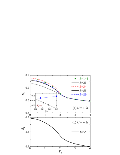
Figure 2: (Color online) The ground-state energy of repulsive (a) and attractive polarons (b) as a function of the disorder strength, at the interaction strength $\left|U\right|=2t$. In (a), we check the dependence of the polaron energy on the length of the system. The inset shows the $1/L$ dependence of the polaron energy at a weak disorder strength $V_{0}=t$. By extrapolating to $1/L=0$, we obtain $E_{P}(V_{0}=t)\simeq 0.744t$ in the thermodynamic limit. In contrast, in the localized phase, the length dependence is extremely weak. The average filling factor of fermionic atoms is $\left\langle\hat{n}\right\rangle=1/2$.

Figure 2 reports the energy of the ground-state polaron at an intermediate onsite interaction strength $\left|U\right|=2t$ for the system length up to $L=144$. Both the energy of repulsive and attractive polarons decreases with increasing quasi-random disorder strength. However, the length dependence of the polaron energy is very different for weak and strong disorder. In the former case, the finite-size effect is pronounced. Numerically we find that the finite-size correction to energy is approximately proportional to $1/L$, as shown in the inset at the disorder strength $V_{0}=t$, with a coefficient that depends on the parity of the length. Thus, the polaron energy approach its thermodynamic limit from above or below for even or odd system length, respectively. In contrast, at strong disorder (i.e., $V_{0}>2t$), the polaron energy essentially does not depend on the length.

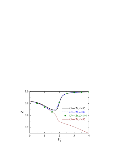
Figure 3: (Color online) The residue of repulsive (thick solid line, dashed line and circles) and attractive polarons (thin solid line) as a function of the disorder strength, at the interaction strength $\left|U\right|=2t$. We take an average filling factor of fermionic atoms $\left\langle\hat{n}\right\rangle=1/2$.

The residue of the ground-state polaron similarly shows different length dependence at weak and strong disorder, as illustrated in Fig. 3. Furthermore, it is interesting that the behavior of the residue is also affected by the sign of the impurity-atom interaction. While the residues of both repulsive and attractive polarons initially decrease with increasing disorder strength, beyond a threshold $V_{0,c}\thicksim 2t$, the residue of the repulsive polaron saturates to unity and that of the attractive polaron continues to decrease. Therefore, for a repulsive polaron, the impurity will finally be isolated by strong disorder. In contrast, for an attractive polaron, the impurity will bind more tightly with surrounding fermionic atoms in the strong disorder limit. In other words, the formation of a molecule is favored at strong disorder.

III.2 Localization of the ground-state polaron

The different finite-size dependence of the polaron energy and residue at weak and strong disorder indicates that there is a localization transition of the ground-state polaron, which we now characterize quantitatively by using the IPR.

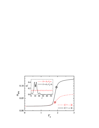
Figure 4: (Color online) The inverse participation ratio of repulsive (solid line) and attractive polarons (dashed line) as a function of the disorder strength, at the interaction strength $\left|U\right|=2t$. The circles indicate the inflection point of the curve (i.e., the threshold for the localization of the ground-state polaron). The inset shows the wave-function of the ground-state polaron $\psi_{i}$ at $\theta=2\pi/5$. The other parameters are the same as in Fig. 3.

Figure 4 presents the disorder dependence of $\alpha_{\text{IPR}}$ of repulsive and attractive polarons at the interaction strength $\left|U\right|=2t$. As anticipated, there is a sharp increase at about $V_{0}\thicksim 2t$. We then identify $V_{0,c}$ as the inflection point of the calculated curve $\alpha_{\text{IPR}}(V_{0})$ Dufour2012 , as indicated by the circle symbol. We have checked that the threshold $V_{0,c}$ is independent on the choice of the phase offset $\theta$. With increasing disorder strength across $V_{0,c}$, the wave-function of polaron (impurity) must change from extended to exponentially localized. To see this, we show in the inset the wave-function of an attractive polaron in the extended phase ($V_{0}=t$) and of a repulsive polaron in the localized phase ($V_{0}=3t$). We emphasize that the observed localization of the polaron wave-function is induced by the impurity-atom interaction, since the impurity itself does not experience the quasi-disorder disorder potential. By repeating the calculation of $\alpha_{\text{IPR}}$ for different interaction strengths, we determine the phase boundary for the localization of the ground-state polaron, as shown in the phase diagram Fig. 1 by solid circles.

III.3 Many-body localization of all polaron states

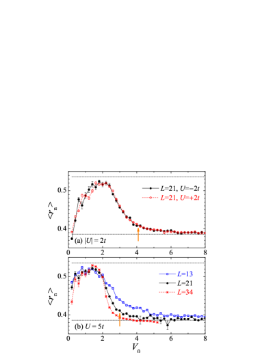
Figure 5: (Color online) Averaged ratio of adjacent energy gaps as a function of the disorder strength for three values of the interaction strength $\left|U\right|=2t$ (a) and $U=5t$ (b). The average $\left\langle r_{n}\right\rangle$ was calculated over the central half of the spectrum, averaging over $20-200$ quasi-random disorder realizations by choosing randomly the phase offset $\theta$. In (a), we check that the average ratio is independent on the sign of the interaction strength. In (b), we show the length dependence of the average ratio. The arrows indicate the estimated critical disorder strength (see text), at which the many-body localization of all polaron states occurs. The two thin dot-dashed lines show the average ratio for the Wigner-Dyson distribution ($\left\langle r_{n}\right\rangle_{\textrm{WD}}\simeq 0.536$) and for the Poisson distribution ($\left\langle r_{n}\right\rangle_{\textrm{P}}\simeq 0.386$).

We now turn to consider the MBL of all polaron states by computing the averaged ratio of adjacent energy levels. In Fig. 5, we show the ratio at the interaction strengths $\left|U\right|=2t$ (a) and $U=5t$ (b), as a function of the disorder strength. For any interaction strength, the disorder dependence of the ratio is similar: at very weak disorder the ratio approximately takes the value $\left\langle r_{n}\right\rangle_{\textrm{P}}\simeq 0.386$ (i.e., the phase I), at some intermediate disorder strengths the ratio increases to about $\left\langle r_{n}\right\rangle_{\textrm{WD}}\simeq 0.536$ (the phase II), and at strong disorder the ratio crosses over to $\left\langle r_{n}\right\rangle_{\textrm{P}}$ again (the phase III). The area of the phase I shrinks quickly by increasing the absolute value of the interaction strength.

The existence of the phase I can be easily understood from the clean limit, where the system becomes integrable (or exactly solvable by Bethe ansatz) McGuire1965 ; McGuire1966 and thus loses its ability to thermalize. The Poisson distribution can be understood as a result of the localization of the system in momentum space. In contrast, in the phase III at strong disorder, the system becomes localized in real space. In between, the system has extended wave-functions in real space and has the ability to reach thermal equilibrium against perturbations.

It is readily seen from Fig. 5(a) that the averaged ratio and hence the MBL do not depend on the sign of the impurity-atom interaction. The same sign-independence has been experimentally observed for the localization of a charge-density-wave state Schreiber2015 . On the other hand, the averaged ratio depends on the length of the system, as explicitly shown in Fig. 5(b) for $U=5t$. A larger system have more Poisson-like statistics than a smaller one for strong disorder in the apparent localized regime, i.e. $V_{0}>3t$ Oganesyan2007 . The size dependence of the ratio, however, becomes weak for a relatively large $L$. In our calculations, we thus estimate the critical disorder strength of MBL by using the criterion,

$$\left\langle r_{n}\right\rangle_{L=21}\left(V_{0,c}\right)=0.41.$$ (23)

The uncertainty of this estimation, $\delta V_{0,c}$, can be similarly determined using the condition, $\left\langle r_{n}\right\rangle_{L=21}\left(V_{0,c}-\delta V_{0,c}\right)=0.43.$ In the figure, the critical disorder strength determined in this manner has been indicated by the arrow. By repeating the same calculation for different interaction strengths, we obtain the MBL critical disorder strength, as reported in the phase diagram Fig. 1 by empty squares.

IV Conclusions and outlooks

In summary, we have investigated the many-body localization phenomenon in the simplest cold-atom setup: a Fermi polaron in quasi-random optical lattices, where the localization is induced by the impurity-atom interaction. The use of Chevy’s variational approach enables us to access relatively large samples and therefore we have approximately determined a phase diagram of many-body localization in the thermodynamic limit. The localization of the ground-state polaron has also been studied in greater detail. While at weak disorder both attractive and repulsive polarons in the ground state behave similarly, at strong disorder the impurity in an attractive polaron binds with atoms to form a molecule and the impurity in a repulsive polaron is isolated from atoms. We note that, both the energy and wave-function of the ground-state polaron can be experimentally determined by using radio-frequency spectroscopy and quantum gas microscope, respectively. The ground-state localization can therefore be directly observed.

Our variational ansatz can be easily generalized to take into account the effect of the external harmonic trapping potential in real experiments. Moreover, to improve the quality of the ansatz, we may also consider two particle-hole excitations and use the ansatz

$$\left|\text{P2}\right\rangle=\left[\sum\limits_{n}z_{n}d_{n}^{\dagger}+\sum\limits_{n,\eta_{h},\eta_{p}}\alpha_{n}\left(\eta_{h},\eta_{p}\right)\hat{d}_{n}^{\dagger}\hat{c}_{\eta_{p}}^{\dagger}\hat{c}_{\eta_{h}}+\sum\limits_{n,\eta_{h1},\eta_{h2,}\eta_{p1},\eta_{p2}}\alpha_{n}\left(\eta_{h1},\eta_{h2},\eta_{p1},\eta_{p2}\right)\hat{d}_{n}^{\dagger}\hat{c}_{\eta_{p2}}^{\dagger}\hat{c}_{\eta_{p1}}^{\dagger}\hat{c}_{\eta_{h2}}\hat{c}_{\eta_{h1}}\right]\left|\text{FS}\right\rangle.$$ (24)

The number of possible states in the enlarged Hilbert space is about $L^{5}/64$. Therefore, we have $D_{l=6}\simeq 5,801$, $D_{l=7}\simeq 63,814$, and $D_{l=8}\simeq 709,928$. We may address the polaron problem with improved accuracy for $l$ up to $8$ and $L=F_{l}$ up to $34$.

- (1) R. Nandkishore and D. A. Huse, Ann. Rev. Condens. Matter Phys. 6, 15 (2015).
- (2) E. Altman and R. Vosk, Ann. Rev. of Condens. Matter Phys. 6, 383 (2015).
- (3) D. M. Basko, I. L. Aleiner, and B. L. Altshuler, Ann. Phys. 321, 1126 (2006).
- (4) I. L. Aleiner, B. L. Altshuler, and G. V. Shlyapnikov, Nature Phys. 6, 900 (2010).
- (5) V. Oganesyan and D. A. Huse, Phys. Rev. B 75, 155111 (2007).
- (6) A. Pal and D. A. Huse, Phys. Rev. B 82, 174411 (2010).
- (7) J. H. Bardarson, F. Pollmann, and J. E. Moore, Phys. Rev. Lett. 109, 017202 (2012).
- (8) R. Mondaini and M. Rigol, Phys. Rev. A 92, 041601(R) (2015).
- (9) M. Schreiber, S. S. Hodgman, P. Bordia, H. P. Lüschen, M. H. Fischer, R. Vosk, E. Altman, U. Schneider, and I. Bloch, Science 349, 842 (2015).
- (10) P. Bordia, H. P. Lüschen, S. S Hodgman, M. Schreiber, I. Bloch, and U. Schneider, arXiv:1509.00478 (2015).
- (11) P. G. Harper, Proc. Phys. Soc. London Sect. A 68, 874 (1955).
- (12) S. Aubry and G. André, Ann. Isr. Phys. Soc. 3, 133 (1980).
- (13) I. Bloch, J. Dalibard, and W. Zwerger, Rev. Mod. Phys. 80, 885 (2008).
- (14) F. Evers and A. D. Mirlin, Rev. Mod. Phys. 80, 1355 (2008).
- (15) F. Chevy, Phys. Rev. A 74, 063628 (2006).
- (16) C. Lobo, A. Recati, S. Giorgini, and S. Stringari, Phys. Rev. Lett. 97, 200403 (2006).
- (17) A. Schirotzek, C.-H. Wu, A. Sommer, and M. W. Zwierlein, Phys. Rev. Lett. 102, 230402 (2009).
- (18) A. N. Wenz, G. Zürn, S. Murmann, I. Brouzos, T. Lompe, and S. Jochim, Science 342, 457 (2013).
- (19) P. Massignan, M. Zaccanti, and G. M. Bruun, Rep. Prog. Phys. 77, 034401 (2014).
- (20) L. W. Cheuk, M. A. Nichols, M. Okan, T. Gersdorf, V. V. Ramasesh, W. S. Bakr, T. Lompe, and M. W. Zwierlein, Phys. Rev. Lett. 114, 193001 (2015).
- (21) M. F. Parsons, F. Huber, A. Mazurenko, C. S. Chiu, W. Setiawan, K. Wooley-Brown, S. Blatt, M. Greiner, Phys. Rev. Lett. 114, 213002 (2015).
- (22) A. Omran, M. Boll, T. Hilker, K. Kleinlein, G. Salomon, I. Bloch, and C. Gross, arXiv:1510.04599 (2015).
- (23) E. V. H. Doggen, A. Korolyuk, P. Törmä, and J. J. Kinnunen, Phys. Rev. A 89, 053621 (2014).
- (24) M. Kohmoto, Phys. Rev. Lett. 51, 1198 (1983).
- (25) G. Dufour and G. Orso, Phys. Rev. Lett. 109, 155306 (2012).
- (26) J. B. McGuire, J. Math. Phys. 6, 432 (1965).
- (27) J. B. McGuire, J. Math. Phys. 7, 123 (1966).