SUPERHORIZON MAGNETIC FIELDS

Abstract

We analyze the evolution of superhorizon-scale magnetic fields from the end of inflation till today. Whatever is the mechanism responsible for their generation during inflation, we find that a given magnetic mode with wave number $k$ evolves, after inflation, according to the values of $k\eta_{e}$, $n_{\mathbf{k}}$, and $\Omega_{k}$, where $\eta_{e}$ is the conformal time at the end of inflation, $n_{\mathbf{k}}$ is the number density spectrum of inflation-produced photons, and $\Omega_{k}$ is the phase difference between the two Bogolubov coefficients which characterize the state of that mode at the end of inflation. For any realistic inflationary magnetogenesis scenario, we find that $n_{\mathbf{k}}^{-1}\ll|k\eta_{e}|\ll 1$, and three evolutionary scenarios are possible: ($i$) $|\Omega_{k}\mp\pi|=\mathcal{O}(1)$, in which case the evolution of the magnetic spectrum $B_{k}(\eta)$ is adiabatic, $a^{2}B_{k}(\eta)=\mbox{const}$, with $a$ being the expansion parameter; ($ii$) $|\Omega_{k}\mp\pi|\ll|k\eta_{e}|$, in which case the evolution is superadiabatic, $a^{2}B_{k}(\eta)\propto\eta$; ($iii$) $|k\eta_{e}|\ll|\Omega_{k}\mp\pi|\ll 1$ or $|k\eta_{e}|\sim|\Omega_{k}\mp\pi|\ll 1$, in which case an early phase of adiabatic evolution is followed, after a time $\eta_{\star}\sim|\Omega_{k}\mp\pi|/k$, by a superadiabatic evolution. Once a given mode reenters the horizon, it remains frozen into the plasma and then evolves adiabatically till today. As a corollary of our results, we find that inflation-generated magnetic fields evolve adiabatically on all scales and for all times in conformal-invariant free Maxwell theory, while they evolve superadiabatically after inflation on superhorizon scales in the nonconformal-invariant Ratra model, where the inflaton is kinematically coupled to the electromagnetic field. The latter result supports and, somehow, clarifies our recent claim that the Ratra model can account for the presence of cosmic magnetic fields without suffering from both backreaction and strong-coupling problems.

I I. Introduction

Recent astrophysical observations of gamma-rays spectra of distant blazars Neronov-Vovk ; Tavecchio1 ; Tavecchio2 ; Caprini0 strongly indicate the presence of large-scale magnetic fields in cosmic voids. Together with the ubiquitous presence of large-scale, coherent magnetic fields in clusters of galaxies and the magnetization of galaxies at both low and high redshifts, this fact strongly points toward ($i$) the existence of a “cosmic magnetic field” that pervades the entire observable universe, ($ii$) that its origin is primordial (namely, it took place before large-scale structures formation), and ($iii$) it is a relic of inflation (for reviews on primordial magnetic fields, see Widrow ; Giovannini ; Tsagas ; Widrow2 ; Durrer ; Subra ).

However, because of the conformal invariance of classical Maxwell electromagnetism in a Friedmann-Robertson-Walker background, photons cannot be created during inflation, as a consequence of the “Parker theorem” Birrell-Davies ; Parker-Toms . Quantum effects, nevertheless, can break such a conformal invariance allowing for a generation of strong magnetic fields Dolgov ; Campanelli , or electromagnetic vacuum fluctuations can either survive and be amplified in marginally open universes Tsagas-Kandus ; Barrow-Tsagas ; Barrow-et al , or be “boosted” by gravitational waves TsagasGW .

Another possibility to create seed magnetic fields during inflation is to consider nonstandard, nonconformal-invariant electromagnetic theories. Starting from the seminal papers by Turner and Widrow Turner-Widrow , who studied nonconformal couplings between photons and gravity, and by Ratra Ratra , who considered a conformal-breaking coupling between the inflaton and the electromagnetic field, there have been many attempts in this direction (see, e.g., G1 ; G2 ; G3 ; G4 ; G5 ; G6 ; G7 ; G8 ; G9 ; G10 ; G11 ; G12 ; G13 ; G14 ; G15 ; G16 ; G17 ; G18 ; G19 ; G20 ; G21 ; G22 ; G23 ; G24 ; G25 ; G26 ; G27 ; G28 ; G29 ; G30 ; G31 ; G32 ; G33 ; G34 ; G35 ; G36 ; G37 ).

After the work Demozzi , all these attempts in constructing models of inflationary magnetogenesis have been believed to be untrustful because of the so-called “strong coupling problem” and “backreaction problem,” and efforts have been made in constructing successful scenarios in which both problems are avoided Ferreira ; Membiela ; Subramanian1 ; Caprini ; Subramanian2 ; Tasinato ; Campanelli2 ; Sasaki ; Guo-Qian .

Recently enough Campanelli1 , however, we have stressed the fact that there is a flaw in the arguments of Demozzi and in the proposed nonstandard magnetogenesis mechanisms. There, in fact, it is assumed that, after reheating, postinflationary electric currents froze inflation-produced superhorizon magnetic fields. But this implies a violation of causality since, as first pointed out in Barrow-Tsagas , postinflationary currents are generated by microphysical processes during reheating and, then, are vanishing on superhorizon scales. Fixing the “causality flaw” in the Ratra model by studying the creation of photons out from the vacuum via the “Parker mechanism” Birrell-Davies ; Parker-Toms , we have found that the Ratra model is a viable, and indeed successful, scenario of inflationary magnetogenesis.

The implications for cosmic magnetogenesis of having vanishing superhorizon electric currents have been investigated by Tsagas Tsagas1 . He analyzed the case of free Maxwell theory in flat, marginally open, and marginally closed universes, and a particular case of nonstandard electromagnetism, the one where magnetic fields during inflation evolve as a power of the expansion parameter, $B\propto a^{-m}$ with $0\leq m<2$ (the latter case has been further developed in Tsagas2 ). The result is that, in general, superhorizon magnetic fields do not evolve adiabatically after reheating.

The aim of this paper is threefold. First, we will show that quantum magnetic fluctuations in Maxwell theory evolve adiabatically in a spatially flat universe once the Bunch-Davies vacuum is chosen to be the physical vacuum state. Second, we will generalize the results in Tsagas2 by studying the postinflationary evolution of superhorizon magnetic fields in a general nonconformal-invariant electromagnetic theory. Third, we will show that inflation-produced, superhorizon magnetic fields are superadiabatically amplified after inflation in the Ratra model, thus supporting our recent claim that the Ratra model evades both the backreaction and strong-coupling problems.

II II. Free Maxwell Theory

In this section, we analyze the evolution of magnetic fields in free Maxwell theory. We use two equivalent approaches, the “photon wave function” and the “magnetic flux” approaches. These will also be used in the next section when we study the case of nonconformal-invariant theories. While the first approach is, in our opinion, more direct, the second one is useful when comparing our results with those of Tsagas1 ; Tsagas2 .

II.1 IIa. Photon wave function approach

Let us consider the free Maxwell theory described by the Lagrangian ${\mathcal{L}}_{\rm em}=-\frac{1}{4}F_{\mu\nu}F^{\mu\nu}$, where $F_{\mu\nu}=\partial_{\mu}A_{\nu}-\partial_{\nu}A_{\mu}$, and $A_{\mu}$ is the photon field. We restrict our analysis to the case of a spatially flat, Friedmann-Robertson-Walker universe, described by the line element

$$ds^{2}=a^{2}(d\eta^{2}-d\mathbf{x}^{2}),$$ (1)

where $\eta$ is the conformal time and $a(\eta)$ is the expansion parameter, which we normalize to unity at the present time $\eta_{0}$. Working in the Coulomb gauge, $A_{0}=\partial_{i}A_{i}=0$, we quantize the electromagnetic field by expanding it, in the Fock space, as

$${\mathbf{A}}(\eta,\mathbf{x})=\sum_{\alpha=1,2}\int\!\!\frac{d^{3}k}{(2\pi)^{3}\sqrt{2k}}\,a_{\mathbf{k},\alpha}\,A_{k,\alpha}(\eta)\,{\bm{\varepsilon}}_{\mathbf{k},\alpha}\,e^{i\mathbf{k}\mathbf{x}}+\mbox{H.c.},$$ (2)

where $A_{\mu}=(0,\mathbf{A})$, $\mathbf{k}$ is the comoving wave number, $k=|\mathbf{k}|$, and ${\bm{\varepsilon}}_{\mathbf{k},\lambda}$ are the standard circular polarization vectors. The annihilation and creation operators $a_{\mathbf{k},\alpha}$ and $a_{\mathbf{k},\alpha}^{{\dagger}}$ satisfy the usual commutation relations $[a_{\mathbf{k},\alpha},a_{\mathbf{k}^{\prime},\alpha^{\prime}}^{{\dagger}}]=(2\pi)^{3}\delta_{\alpha\alpha^{\prime}}\delta(\mathbf{k}-\mathbf{k}^{\prime})$, all the other commutators being null. In order to get the usual commutation relations for the electromagnetic field and its canonical conjugate momentum, one must impose the Wronskian condition

$$A_{k,\alpha}A^{\prime*}_{k,\alpha}-A^{*}_{k,\alpha}A^{\prime}_{k,\alpha}=2ik$$ (3)

on the wave functions of the two photon polarization states $A_{k,\alpha}$. (Hereafter, a prime indicates a differentiation with respect to the conformal time.) Finally, the vacuum state $|0\rangle$ is defined by $a_{\mathbf{k},\lambda}|0\rangle=0$ for all $\mathbf{k}$ and $\alpha$ and normalized as $\langle 0|0\rangle=1$. The photon wave functions satisfy the usual free harmonic oscillator equation,

$$A_{k,\alpha}^{\prime\prime}+k^{2}A_{k,\alpha}=0,$$ (4)

whose solution is

$$A_{k,\alpha}(\eta)=c_{1,\alpha}(k)\,e^{-ik\eta}+c_{2,\alpha}(k)\,e^{ik\eta}.$$ (5)

Here, $c_{1,\alpha}(k)$ and $c_{2,\alpha}(k)$ are integration constants which are fixed by the choice of the vacuum. The Wronskian condition implies that

$$|c_{1,\alpha}(k)|^{2}-|c_{2,\alpha}(k)|^{2}=1.$$ (6)

The physical vacuum is the so-called Bunch-Davies vacuum Birrell-Davies defined by

$$c_{1,\alpha}(k)=1\,,\;\;\;c_{2,\alpha}(k)=0.$$ (7)

Accordingly, the photon wave functions, in free Maxwell theory, are the usual plane waves

$$A_{k,\alpha}(\eta)=e^{-ik\eta}.$$ (8)

Let us now introduce the magnetic field as usual as $a^{2}\mathbf{B}=\nabla\times\mathbf{A}$. The observable quantity is the vacuum expectation value (VEV) of the squared magnetic field operator. Using Eq. (2), we find

$$\langle 0|\mathbf{B}^{2}(\eta,\mathbf{x})|0\rangle=\int_{0}^{\infty}\!\frac{dk}{k}\,B_{k}^{2}(\eta),$$ (9)

where

$$B_{k}^{2}(\eta)=\frac{k^{4}}{4\pi^{2}a^{4}}\sum_{\alpha=1,2}|A_{k,\alpha}(\eta)|^{2}$$ (10)

is the so-called magnetic power spectrum, and $B_{k}(\eta)$ the magnetic field on the scale $1/k$. Inserting Eq. (5) in Eq. (10), and taking into account Eq. (7), we find

$$a^{2}B_{k}(\eta)=\frac{k^{2}}{\sqrt{2}\pi}\,,$$ (11)

which shows that, in free Maxwell theory, magnetic fields evolve adiabatically (i.e., proportionally to $a^{-2}$) for all times.

The introduction of the conductivity does not change this result. In fact, its only effect, due to his huge value in the early universe, is to force subhorizon magnetic fields to evolve adiabatically after reheating. Accordingly, magnetic fields that evolve adiabatically before reheating will keep evolving adiabatically till today.

II.2 IIb. Magnetic flux approach

The “magnetic flux” is defined by ${\bm{\mathcal{B}}}(\eta,\mathbf{x})=a^{2}\mathbf{B}(\eta,\mathbf{x})$. In Fock space, we have

$${{\bm{\mathcal{B}}}}(\eta,\mathbf{x})=\sum_{\alpha=1,2}\int\!\!\frac{d^{3}k}{(2\pi)^{3}\sqrt{2k}}\,a_{\mathbf{k},\alpha}\,{\bm{\mathcal{B}}}_{\mathbf{k},\alpha}(\eta)\,e^{i\mathbf{k}\mathbf{x}}+\mbox{H.c.},$$ (12)

where we have defined

$${\bm{\mathcal{B}}}_{\mathbf{k},\alpha}=k(-1)^{\alpha+1}A_{k,\alpha}(\eta){\bm{\varepsilon}}_{\mathbf{k},\alpha}.$$ (13)

Summing up the two photon polarization states, $\sum_{\alpha=1,2}{\bm{\mathcal{B}}}_{\mathbf{k},\alpha}$, we get the Fourier transform of the magnetic flux. However, it is more useful to introduce the quantity

$$a^{2}\mathbf{B}_{\mathbf{k}}={\bm{\mathcal{B}}}_{\mathbf{k}}=\frac{k}{2\pi}\sum_{\alpha=1,2}{\bm{\mathcal{B}}}_{\mathbf{k},\alpha}$$ (14)

(which we will still call Fourier transform of the magnetic flux for the sake of convenience), for two reasons. First, it has the dimension of a magnetic field and, second, because

$$|\mathbf{B}_{\mathbf{k}}(\eta)|=B_{k}(\eta),$$ (15)

namely, the modulus of the Fourier-transformed magnetic field is equal to the magnetic field on the scale $1/k$.

The Fourier transform of the magnetic flux satisfies, in the hypothesis of null conductivity, the field equation

$${\bm{\mathcal{B}}}^{\prime\prime}_{\mathbf{k}}+k^{2}{\bm{\mathcal{B}}}_{\mathbf{k}}=0,$$ (16)

whose solution is

$${\bm{\mathcal{B}}}_{\mathbf{k}}=a^{2}\mathbf{B}_{\mathbf{k}}={\bm{\mathcal{C}}}_{1}\cos(k\eta)+{\bm{\mathcal{C}}}_{2}\sin(k\eta),$$ (17)

where ${\bm{\mathcal{C}}}_{1}(\mathbf{k})$ and ${\bm{\mathcal{C}}}_{2}(\mathbf{k})$ are complex constant vectors of integration. Inserting Eq. (5) in Eq. (13), and comparing the resulting expression with Eq. (17), we get

$${\bm{\mathcal{C}}}_{1}=\frac{k^{2}}{2\pi}\sum_{\alpha}(-1)^{\alpha+1}[c_{1,\alpha}(k)+c_{2,\alpha}(k)]{\bm{\varepsilon}}_{\mathbf{k},\alpha},$$ (18)

$${\bm{\mathcal{C}}}_{2}=-i\frac{k^{2}}{2\pi}\sum_{\alpha}(-1)^{\alpha+1}[c_{1,\alpha}(k)-c_{2,\alpha}(k)]{\bm{\varepsilon}}_{\mathbf{k},\alpha}.$$ (19)

The Wronskian condition (3) on the photon wave function implies that

$${\bm{\mathcal{C}}}_{1}\cdot{\bm{\mathcal{C}}}_{2}^{*}-{\bm{\mathcal{C}}}_{1}^{*}\cdot{\bm{\mathcal{C}}}_{2}=\frac{ik^{4}}{\pi}\,.$$ (20)

Equations (18)-(19) show that the integration constants ${\bm{\mathcal{C}}}_{1}$ and ${\bm{\mathcal{C}}}_{2}$ are fixed by the choice of the vacuum. The (physical) Bunch-Davies vacuum is defined by Eq. (7), and then it corresponds to take

$${\bm{\mathcal{C}}}_{1}=\frac{k^{2}}{2\pi}\left({\bm{\varepsilon}}_{\mathbf{k},1}-{\bm{\varepsilon}}_{\mathbf{k},2}\right),\;\;\;{\bm{\mathcal{C}}}_{2}=-i{\bm{\mathcal{C}}}_{1}.$$ (21)

Inserting the above relations in Eq. (17), we get

$$a^{2}\mathbf{B}_{\mathbf{k}}(\eta)={\bm{\mathcal{C}}}_{1}e^{-ik\eta},$$ (22)

from which it follows that $|a^{2}\mathbf{B}_{\mathbf{k}}(\eta)|=k^{2}/\sqrt{2}\pi$, in agreement with Eq. (11).

To compare our results with those in Tsagas1 , let us rewrite Eq. (17) in the long wavelength limit (namely, for superhorizon modes, $|k\eta|\ll 1$),

$$a^{2}\mathbf{B}_{\mathbf{k}}\simeq{\bm{\mathcal{C}}}_{1}+{\bm{\mathcal{C}}}_{2}k\eta.$$ (23)

From the above equation, it follows that the constant ${\bm{\mathcal{C}}}_{1}$ and ${\bm{\mathcal{C}}}_{2}$ can be expressed as a function of $\mathbf{B}_{\mathbf{k}}$ and its first derivative calculated at a reference time $\eta_{*}$:

$${\bm{\mathcal{C}}}_{1}\simeq-[(2\eta\mathcal{H}-1)\mathbf{B}_{\mathbf{k}}+\eta\mathbf{B}_{\mathbf{k}}^{\prime}]\,a^{2}|_{\eta=\eta_{*}},$$ (24)

$${\bm{\mathcal{C}}}_{2}\simeq[2\eta\mathcal{H}\mathbf{B}_{\mathbf{k}}+\eta\mathbf{B}_{\mathbf{k}}^{\prime}]\,\frac{a^{2}}{k\eta}|_{\eta=\eta_{*}},$$ (25)

where $\mathcal{H}=a^{\prime}/a$. Now the author of Tsagas1 argues that, since ${\bm{\mathcal{C}}}_{2}$ is inversely proportional to $k\eta_{*}$, then $|{\bm{\mathcal{C}}}_{2}|\gg|{\bm{\mathcal{C}}}_{1}|$, unless the quantity $2\eta\mathcal{H}\mathbf{B}_{\mathbf{k}}+\eta\mathbf{B}_{\mathbf{k}}^{\prime}$ is null. Consequently, the dominant term in Eq. (23) would be the nonadiabatic one (namely that proportional to ${\bm{\mathcal{C}}}_{2}$), and this would open the possibility to have a superadiabatic evolution of magnetic fields in the free Maxwell theory. However, this does not happen in a theory based on the Bunch-Davies vacuum since the quantity $2\eta\mathcal{H}\mathbf{B}_{\mathbf{k}}+\eta\mathbf{B}_{\mathbf{k}}^{\prime}$ is, in this case, null at the lowest order in $|k\eta|\ll 1$. In fact, from Eq. (22), it follows that

$$2\eta\mathcal{H}\mathbf{B}_{\mathbf{k}}+\eta\mathbf{B}_{\mathbf{k}}^{\prime}=-ik\eta\mathbf{B}_{\mathbf{k}}.$$ (26)

When inserted in Eqs. (24)-(25), the above equation gives ${\bm{\mathcal{C}}}_{1}\simeq i{\bm{\mathcal{C}}}_{2}\simeq a^{2}\mathbf{B}_{\mathbf{k}}|_{\eta=\eta_{*}}$, which shows that $|{\bm{\mathcal{C}}}_{1}|$ and $|{\bm{\mathcal{C}}}_{2}|$ are constants of the same magnitude and, in turn, that the magnetic field evolves adiabatically on superhorizon scales. Finally, for the sake of completeness, we observe that the exact result is

$${\bm{\mathcal{C}}}_{1}=i{\bm{\mathcal{C}}}_{2}=e^{ik\eta}a^{2}\mathbf{B}_{\mathbf{k}}|_{\eta=\eta_{*}}.$$ (27)

III III. Nonconformal-invariant theories

Let us now consider the case where electromagnetic fields during inflation are described by a (nonstandard) nonconformal-invariant electromagnetic Lagrangian. After inflation, instead, we assume that such a Lagrangian smoothly reduces to the Maxwell Lagrangian in order to recover standard electromagnetism and not to spoil, thus, the predictions of the standard cosmological model.

III.1 IIIa. Photon wave function approach

Since photons after inflation are described by the standard free electromagnetism, they evolve according to Eq. (5), with $c_{1,\alpha}(k)$ and $c_{2,\alpha}(k)$ being complex functions of $k$ that are fixed by the properties of the electromagnetic field at the end of inflation. Let us assume, for the sake of simplicity, that the dynamics of the electromagnetic field during inflation is parity conserving, so that $c_{1,\alpha}(k)$ and $c_{2,\alpha}(k)$ do not depend on the photon helicity index $\alpha$:

$$c_{1,\alpha}(k)=\alpha_{k},\;\;\;c_{2,\alpha}(k)=\beta_{k}.$$ (28)

(The parity-violating case, which is associated with the production of magnetic helicity, goes along the same lines as below.) The coefficients $\alpha_{k}$ and $\beta_{k}$ are known as the Bogolubov coefficient, and the Wronskian condition implies the Bogolubov relation

$$|\alpha_{k}|^{2}-|\beta_{k}|^{2}=1.$$ (29)

The square modulus of the coefficient $\beta_{k}$ gives the number (density) of the produced photons during inflation Campanelli1 ,

$$n_{\mathbf{k}}=|\beta_{k}|^{2},$$ (30)

and it is zero for the case of conformal-invariant theories Birrell-Davies , such as the free Maxwell theory in a Friedmann-Robertson-Walker spacetime. Inserting Eq. (5) in Eq. (10), and taking into account Eqs. (28), (29) and (30), we find

$$a^{2}B_{k}(\eta)=\!\frac{k^{2}}{\sqrt{2}\pi}\sqrt{1\!+\!2n_{\mathbf{k}}\!+\!2\sqrt{n_{\mathbf{k}}(n_{\mathbf{k}}\!+\!1)}\cos(\Omega_{k}\!-\!2k\eta)},$$ (31)

where

$$\Omega_{k}=\mbox{Arg}(\alpha_{k}\beta_{k}^{*})\,\in\;]-\pi,\pi]$$ (32)

is the phase difference between the two Bogolubov coefficients. Equation (31) is in agreement with the result of Campanelli1 .

If $n_{\mathbf{k}}=0$ (conformal-invariant theories), then $a^{2}B_{k}(\eta)=k^{2}/\sqrt{2}\pi$, in agreement with the result of Sec. II [see Eq. (11)].

In general, in order to explain the large-scale magnetic fields we observe today in galaxies and clusters of galaxies, we must have $n_{\mathbf{k}}\gg 1$ on scales $\lambda=1/|\mathbf{k}|$ of astrophysical interest for cosmic magnetic fields (see Sec. V). Since we are interested in the evolution of superhorizon modes, let us expand Eq. (31) in the limit $n_{\mathbf{k}}\gg 1$ and $|k\eta|\ll 1$. Independently on the order of the expansion, and to the lowest order, we find

$$a^{2}B_{k}(\eta)\simeq\frac{k^{2}}{\pi}\sqrt{(1+\cos\Omega_{k})n_{\mathbf{k}}}\,.$$ (33)

Therefore, a necessary condition for having a nonadiabatic evolution of superhorizon magnetic fields after inflation is that $\Omega_{k}\rightarrow\pm\pi$ for $n_{\mathbf{k}}\gg 1$. Let us define, for later convenience, the two cases

$$\mbox{case A1}\!:\;\;|\Omega_{k}\mp\pi|=\mathcal{O}(1)\;\;\mbox{and}\;\;n_{\mathbf{k}}^{-1}\ll|k\eta|\ll 1,$$

$$\mbox{case A2}\!:\;\;|\Omega_{k}\mp\pi|=\mathcal{O}(1)\;\;\mbox{and}\;\;|k\eta|\ll n_{\mathbf{k}}^{-1}\ll 1.$$

When cases A1 and A2 are realized, the evolution is then adiabatic.

Let us now consider superhorizon modes such that $\Omega_{k}\rightarrow\pm\pi$ for $n_{\mathbf{k}}\gg 1$. We have six cases: $n_{\mathbf{k}}^{-1}\ll|\Omega_{k}\mp\pi|\ll|k\eta|$ and cyclic permutations. After expanding Eq. (31), we have, to the lowest order,

$$a^{2}B_{k}(\eta)\simeq\frac{k^{2}}{\sqrt{2}\pi}\times\left\{\begin{array}[]{lll}2\sqrt{n_{\mathbf{k}}}\,|k\eta|,&\mbox{B1, B2},\\ |\Omega_{k}\mp\pi|\sqrt{n_{\mathbf{k}}}\,,&\mbox{C1, C2},\\ \frac{1}{2}\sqrt{1/n_{\mathbf{k}}},&\mbox{D1, D2},\end{array}\right.$$ (35)

where the six cases, B1, B2, C1, C2, D1, and D2, correspond to

$$\mbox{case B1}\!:\;\;n_{\mathbf{k}}^{-1}\ll|\Omega_{k}\mp\pi|\ll|k\eta|\ll 1,$$

$$\mbox{case B2}\!:\;\;|\Omega_{k}\mp\pi|\ll n_{\mathbf{k}}^{-1}\ll|k\eta|\ll 1,$$

$$\mbox{case C1}\!:\;\;n_{\mathbf{k}}^{-1}\ll|k\eta|\ll|\Omega_{k}\mp\pi|\ll 1,$$

$$\mbox{case C2}\!:\;\;|k\eta|\ll n_{\mathbf{k}}^{-1}\ll|\Omega_{k}\mp\pi|\ll 1,$$

$$\mbox{case D1}\!:\;\;|\Omega_{k}\mp\pi|\ll|k\eta|\ll n_{\mathbf{k}}^{-1}\ll 1,$$

$$\mbox{case D2}\!:\;\;|k\eta|\ll|\Omega_{k}\mp\pi|\ll n_{\mathbf{k}}^{-1}\ll 1,$$

respectively. Looking at Eq. (35), we conclude that the evolution of superhorizon magnetic fields is superadiabatic, $a^{2}B_{k}(\eta)\propto\eta$, only in the cases B1 and B2, while it is adiabatic in the remaining cases.

Let us now follow the evolution of superhorizon magnetic fields from the end of inflation, at $\eta=\eta_{e}<0$, until today. Let us observe that, although the function $a^{2}B_{k}(\eta)$ in Eq. (31) in not an even function of the conformal time, its asymptotic expansions in Eqs. (33) and (35) are. This allows us to simplify the problem and to consider such an evolution from the positive time $|\eta_{e}|$ till the present time $\eta_{0}$.

If a given magnetic mode with wave number $k$ starts his evolution in the case A1, namely if $|\Omega_{k}\mp\pi|=\mathcal{O}(1)$ and $n_{\mathbf{k}}^{-1}\ll|k\eta_{e}|\ll 1$, then as the time passes and $\eta$ grows, it will remain in the case A1 until it reenters the horizon at the time $\eta_{\downarrow}$ defined by $k\eta_{\downarrow}\simeq 1$. After that, its evolution is still adiabatic because of the high conductivity which freezes any subhorizon magnetic field into the primeval plasma. The evolution, then, is adiabatic for all times.

If the magnetic mode starts in the case A2, its evolution will always be adiabatic, although after a time of order $\eta_{\tiny\mbox{A2}\rightarrow\mbox{A1}}\sim 1/kn_{\mathbf{k}}$, it will move from the case A2 to the case A1.

If the magnetic mode starts in either the case B1 or B2, its evolution will be superadiabatic up to the time $\eta_{\downarrow}$ of its reentering the horizon, and from that time on it will evolve adiabatically.

If the magnetic mode starts in the case C1, it will evolve adiabatically up to the time of order $\eta_{\tiny\mbox{C1}\rightarrow\mbox{B1}}\simeq|\Omega_{k}\mp\pi|/2k$, after which it will move in the case B1, and then will evolve superadiabatically up to its reentering the horizon.

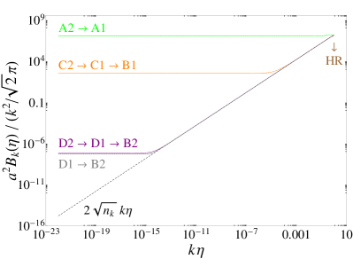
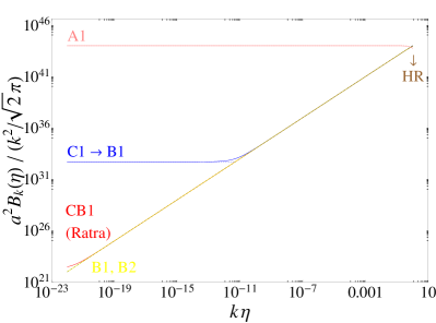
Figure 1: The magnetic flux spectrum, $a^{2}B_{k}(\eta)$, in a nonconformal-invariant theory normalized to its expression in the case of free Maxwell theory, $k^{2}/\sqrt{2}\pi$, as a function of $k\eta$ for different initial conditions at the end of inflation ($\eta=|\eta_{e}|$). For a given magnetic mode $k$, such conditions are determined by the values of $k|\eta_{e}|$, $n_{\mathbf{k}}$, and $\Omega_{k}$, where $n_{\mathbf{k}}$ is the number density of photons created during inflation and $\Omega_{k}$ is the phase difference between the two Bogolubov coefficients which define the state of the magnetic field at the end of inflation. Continuous lines refer to the exact expression of the magnetic flux [see Eq. (31)], while dashed lines to its asymptotic expansions [see Eqs. (33) and (35)]. The cases A1, A2, B1, B2, C1, C2, D1, D2 are defined in Eqs. (III.1) and (III.1), and “HR” stands for “horizon reentering”. Left panel. $k|\eta_{e}|=10^{-22}$ and $n_{\mathbf{k}}=(2/5)^{2}|k\eta_{e}|^{-2/3}$. From top to bottom, $\Omega_{k}=\pi/2$ ($\mbox{A2}\rightarrow\mbox{A1}$), $\Omega_{k}=\pi-|k\eta_{e}|^{1/5}$ ($\mbox{C2}\rightarrow\mbox{C1}\rightarrow\mbox{B1}$), $\Omega_{k}=\pi-2|k\eta_{e}|^{2/3}$ ($\mbox{D2}\rightarrow\mbox{D1}\rightarrow\mbox{B2}$), and $\Omega_{k}=\pi-|k\eta_{e}|^{4}$ ($\mbox{D1}\rightarrow\mbox{B2}$). Right panel. $k|\eta_{e}|=10^{-22}$ and $n_{\mathbf{k}}=(1/4)|k\eta_{e}|^{-4}$. From top to bottom, $\Omega_{k}=0$ (A1), $\Omega_{k}=\pi-|k\eta_{e}|^{1/2}$ ($\mbox{C1}\rightarrow\mbox{B1}$), $\Omega_{k}$ given in Eq. (73) (Ratra model discussed in Sec. IVb), $\Omega_{k}=\pi-|k\eta_{e}|^{3}$ (B1), and $\Omega_{k}=\pi-|k\eta_{e}|^{5}$ (B2).

If a mode starts in the case C2, it will first evolve adiabatically, then it will move from the case C2 to the case C1 at the time $\eta_{\tiny\mbox{C2}\rightarrow\mbox{C1}}\sim 1/kn_{\mathbf{k}}$, then will continue its adiabatic evolution up to the time $\eta_{\tiny\mbox{C1}\rightarrow\mbox{B1}}$, after which it will evolve superadiabatically according to the case B1 until it reenters the horizon.

If the magnetic mode starts in the case D1, it will evolve adiabatically up to the time of order $\eta_{\tiny\mbox{D1}\rightarrow\mbox{B2}}\simeq 1/4kn_{\mathbf{k}}$, after which it will move in the case B2, and then will evolve superadiabatically up to its reentering the horizon.

If a mode starts in the case D2, it will first evolve adiabatically, then it will move from the case D2 to the case D1 at the time $\eta_{\tiny\mbox{D2}\rightarrow\mbox{D1}}\sim|\Omega_{k}\mp\pi|/k$, then will continue its adiabatic evolution up to the time $\eta_{\tiny\mbox{D1}\rightarrow\mbox{B2}}$, after which it will evolve superadiabatically according to the case B2 until it reenters the horizon.

Schematically, the evolution of a given magnetic mode is as follows:

$$\mbox{A1}\rightarrow\mbox{HR}$$

$$\mbox{A2}\rightarrow\mbox{A1}\rightarrow\mbox{HR}$$

$$\mbox{B1}\rightarrow\mbox{HR}$$

$$\mbox{B2}\rightarrow\mbox{HR}$$

$$\mbox{C1}\rightarrow\mbox{B1}\rightarrow\mbox{HR}$$

$$\mbox{C2}\rightarrow\mbox{C1}\rightarrow\mbox{B1}\rightarrow\mbox{HR}$$

$$\mbox{D1}\rightarrow\mbox{B2}\rightarrow\mbox{HR}$$

$$\mbox{D2}\rightarrow\mbox{D1}\rightarrow\mbox{B2}\rightarrow\mbox{HR}$$

where HR stands for horizon reentering.

It is interesting to observe that the actual magnetic field, $B_{k}(\eta_{0})$, which coincides with the magnetic flux at the time of horizon reentering, $a^{2}B_{k}(\eta)|_{\eta=\eta_{\downarrow}}$, is independent of the details of its evolution when outside the horizon. Indeed, from Eq. (31), we find, in the limit $n_{\mathbf{k}}\gg 1$,

$$B_{k}(\eta_{0})\simeq\zeta_{k}k^{2}\sqrt{n_{\mathbf{k}}}\,,$$ (37)

where $\zeta_{k}=\sqrt{1+\cos(\Omega_{k}-2k\eta_{\downarrow})}/\pi$. Since $k\eta_{\downarrow}\simeq 1$ by definition, we see that, excluding a region very near to $\Omega_{k}\simeq 2-\pi$ (where $\zeta_{k}$ is vanishing), $\zeta_{k}$ is an order-one function $\Omega_{k}$. Therefore, the actual magnetic field spectrum is essentially determined by the number of photons with wave number $k$ that have been created during inflation.

In Fig. 1, we show the magnetic flux spectrum $a^{2}B_{k}(\eta)$ normalized to its expression in the case of pure Maxwell theory, $k^{2}/\sqrt{2}\pi$ [see Eq. (11)], as a function of $k\eta$ (with $\eta>0$) for different initial conditions at the end of inflation at $\eta=|\eta_{e}|$. Continuous lines refer to the exact expression of the magnetic flux given in Eq. (31), while dashed lines to its asymptotic expansions given in Eqs. (33) and (35). In both panels, we have taken $k|\eta_{e}|=10^{-22}$. In the left panel, $n_{\mathbf{k}}=(2/5)^{2}|k\eta_{e}|^{-2/3}$ and, from top to bottom, $\Omega_{k}=\pi/2$ ($\mbox{A2}\rightarrow\mbox{A1}$), $\Omega_{k}=\pi-|k\eta_{e}|^{1/5}$ ($\mbox{C2}\rightarrow\mbox{C1}\rightarrow\mbox{B1}$), $\Omega_{k}=\pi-2|k\eta_{e}|^{2/3}$ ($\mbox{D2}\rightarrow\mbox{D1}\rightarrow\mbox{B2}$), and $\Omega_{k}=\pi-|k\eta_{e}|^{4}$ ($\mbox{D1}\rightarrow\mbox{B2}$). In the right panel, $n_{\mathbf{k}}=(1/4)|k\eta_{e}|^{-4}$ and from top to bottom, $\Omega_{k}=0$ (A1), $\Omega_{k}=\pi-|k\eta_{e}|^{1/2}$ ($\mbox{C1}\rightarrow\mbox{B1}$), $\Omega_{k}$ given in Eq. (73) (scaling-invariant case in the Ratra model discussed in Sec. IVb), $\Omega_{k}=\pi-|k\eta_{e}|^{3}$ (B1), and $\Omega_{k}=\pi-|k\eta_{e}|^{5}$ (B2).

III.2 IIIb. Magnetic flux approach

Let us now investigate the evolution of superhorizon magnetic modes using the magnetic flux approach. Taking into account Eq. (28), the coefficients ${\bm{\mathcal{C}}}_{1}$ and ${\bm{\mathcal{C}}}_{2}$ in Eqs. (18) and (19) are

$${\bm{\mathcal{C}}}_{1}=\frac{k^{2}}{2\pi}\,(\alpha_{k}+\beta_{k})\left({\bm{\varepsilon}}_{\mathbf{k},1}-{\bm{\varepsilon}}_{\mathbf{k},2}\right),$$ (38)

$${\bm{\mathcal{C}}}_{2}=-i\frac{k^{2}}{2\pi}\,(\alpha_{k}-\beta_{k})\left({\bm{\varepsilon}}_{\mathbf{k},1}-{\bm{\varepsilon}}_{\mathbf{k},2}\right).$$ (39)

Inserting these expression in Eq. (17), we find

$$a^{2}\mathbf{B}_{\mathbf{k}}(\eta)={\bm{\mathcal{C}}}_{1}\left(\frac{\alpha_{k}}{\alpha_{k}+\beta_{k}}\,e^{-ik\eta}+\frac{\beta_{k}}{\alpha_{k}+\beta_{k}}\,e^{ik\eta}\right)\!,$$ (40)

from which it follows that

$$2\eta\mathcal{H}\mathbf{B}_{\mathbf{k}}+\eta\mathbf{B}_{\mathbf{k}}^{\prime}=-ik\eta\mathbf{B}_{\mathbf{k}}\,g(n_{\mathbf{k}},\Omega_{k},k\eta),$$ (41)

where we have introduced the function

$$g(n_{\mathbf{k}},\Omega_{k},k\eta)=\frac{e^{i(\Omega_{k}-2k\eta)}\sqrt{n_{\mathbf{k}}+1}-\sqrt{n_{\mathbf{k}}}}{e^{i(\Omega_{k}-2k\eta)}\sqrt{n_{\mathbf{k}}+1}+\sqrt{n_{\mathbf{k}}}}\,.$$ (42)

Inserting Eq. (41) in Eqs. (24)-(25), we find

$${\bm{\mathcal{C}}}_{1}\simeq(1+ik\eta g)a^{2}\mathbf{B}_{\mathbf{k}}|_{\eta=\eta_{*}},$$ (43)

$${\bm{\mathcal{C}}}_{2}\simeq-iga^{2}\mathbf{B}_{\mathbf{k}}|_{\eta=\eta_{*}}.$$ (44)

For the eight cases discussed above, we find, to the lowest order,

$$g(n_{\mathbf{k}},\Omega_{k},k\eta)\simeq\left\{\begin{array}[]{lll}i\tan(\Omega_{k}/2),&\mbox{A1, A2}\\ i/k\eta,&\mbox{B1, B2},\\ -2i/(\Omega_{k}\mp\pi),&\mbox{C1, C2},\\ 4n_{\mathbf{k}},&\mbox{D1, D2}.\end{array}\right.$$ (45)

Inserting Eq. (45) in Eqs. (43)-(44), we find

$${\bm{\mathcal{C}}}_{1}\simeq\cot(\Omega_{k}/2)\,{\bm{\mathcal{C}}}_{2}\simeq a^{2}\mathbf{B}_{\mathbf{k}}|_{\eta=\eta_{*}},~{}~{}~{}~{}~{}~{}\,\,\mbox{A1, A2},$$ (46)

$${\bm{\mathcal{C}}}_{1}\simeq 0,\;\;\;{\bm{\mathcal{C}}}_{2}\simeq(k\eta_{*})^{-1}a^{2}\mathbf{B}_{\mathbf{k}}|_{\eta=\eta_{*}},~{}~{}~{}~{}\,\,\mbox{B1, B2},$$ (47)

$${\bm{\mathcal{C}}}_{1}\simeq-[(\Omega_{k}\mp\pi)/2]\,{\bm{\mathcal{C}}}_{2}\simeq a^{2}\mathbf{B}_{\mathbf{k}}|_{\eta=\eta_{*}},~{}\,\mbox{C1, C2},$$ (48)

$${\bm{\mathcal{C}}}_{1}\simeq(i/4n_{\mathbf{k}})\,{\bm{\mathcal{C}}}_{2}\simeq a^{2}\mathbf{B}_{\mathbf{k}}|_{\eta=\eta_{*}},~{}~{}~{}~{}~{}~{}~{}~{}~{}\>\,\mbox{D1, D2}.$$ (49)

The exact expressions for ${\bm{\mathcal{C}}}_{1}$ and ${\bm{\mathcal{C}}}_{2}$ come from the expression of $a^{2}\mathbf{B}_{\mathbf{k}}$ in Eq. (40) evaluated at $\eta=\eta_{*}$ and from Eq. (39). They are:

$${\bm{\mathcal{C}}}_{1}=\frac{a^{2}\mathbf{B}_{\mathbf{k}}|_{\eta=\eta_{*}}}{\cos(k\eta_{*})-ig(n_{\mathbf{k}},\Omega_{k},0)\sin(k\eta_{*})}\,,$$ (50)

$${\bm{\mathcal{C}}}_{2}=-ig(n_{\mathbf{k}},\Omega_{k},0){\bm{\mathcal{C}}}_{1}.$$ (51)

These expressions reduce, in the limit $n_{\mathbf{k}}=0$, to those previously found for the free Maxwell theory [see Eq. (27)]. Inserting Eqs. (46)-(49) in Eq. (23), we find

$$\;\,a^{2}\mathbf{B}_{\mathbf{k}}(\eta)\simeq\!\left\{\begin{array}[]{lll}\!\!a^{2}\mathbf{B}_{\mathbf{k}}|_{\eta=\eta_{*}},&\!\mbox{A1, A2, C1, C2, D1, D2},\\ \!\!a^{2}\mathbf{B}_{\mathbf{k}}|_{\eta=\eta_{*}}\left(\frac{\eta}{\eta_{*}}\right)\!,&\!\mbox{B1, B2}.\end{array}\right.$$ (52)

Finally, observing that $|a^{2}\mathbf{B}_{\mathbf{k}}(\eta)|\simeq|{\bm{\mathcal{C}}}_{1}|$ for the cases A1, A2, C1, C2, D1, and D2, and $|a^{2}\mathbf{B}_{\mathbf{k}}(\eta)|\simeq|{\bm{\mathcal{C}}}_{2}||k\eta|$ for the cases B1, B2, we obtain, at the time $\eta=\eta_{*}$,

$$|a^{2}\mathbf{B}_{\mathbf{k}}|_{\eta=\eta_{*}}\simeq\frac{k^{2}}{\sqrt{2}\pi}\times\left\{\begin{array}[]{lll}\sqrt{2(1+\cos\Omega_{k})n_{\mathbf{k}}}\,,&\mbox{A1, A2},\\ 2\sqrt{n_{\mathbf{k}}}\,|k\eta_{*}|,&\mbox{B1, B2},\\ |\Omega_{k}\mp\pi|\sqrt{n_{\mathbf{k}}}\,,&\mbox{C1, C2},\\ \frac{1}{2}\sqrt{1/n_{\mathbf{k}}},&\mbox{D1, D2},\end{array}\right.$$ (53)

where we used the following asymptotic expansions of ${\bm{\mathcal{C}}}_{1}$ and ${\bm{\mathcal{C}}}_{2}$ in Eqs. (38)-(39): $|{\bm{\mathcal{C}}}_{1}|^{2}\simeq k^{4}(1+\cos\Omega_{k})n_{\mathbf{k}}/\pi^{2}$ for the cases A1, A2; $|{\bm{\mathcal{C}}}_{2}|^{2}\simeq 2k^{4}n_{\mathbf{k}}/\pi^{2}$ for the cases B1, B2; $|{\bm{\mathcal{C}}}_{1}|^{2}\simeq k^{4}(\Omega_{k}\mp\pi)^{2}n_{\mathbf{k}}/2\pi^{2}$ for the cases C1, C2; and $|{\bm{\mathcal{C}}}_{1}|^{2}\simeq k^{4}/8\pi^{2}n_{\mathbf{k}}$ for the cases D1, D2.

Taking the modulus of $a^{2}\mathbf{B}_{\mathbf{k}}(\eta)$ in Eq. (52), and taking into account Eq. (53), we arrive at the same results previously obtained using the photon wave function approach [see Eqs. (33) and (35)].

IV IV. Specific models

We analyze now two specific models of inflationary magnetogenesis. The first one is general enough and just assumes that superhorizon magnetic fields evolve as a power of the conformal time during inflation, while the second one is the well-known Ratra model.

IV.1 IVa. Power-law magnetic fields during inflation

Following Tsagas1 ; Tsagas2 , we rewrite Eqs. (23), (24), and (25) as

$$\mathbf{B}_{\mathbf{k}}(\eta)\!\! = \!\!-[(2\eta\mathcal{H}-1)\mathbf{B}_{\mathbf{k}}+\eta\mathbf{B}_{\mathbf{k}}^{\prime}]_{\eta=\eta_{e}}\left(\frac{a_{e}}{a}\right)^{\!2}$$ (54)

$$+ \!\![2\eta\mathcal{H}\mathbf{B}_{\mathbf{k}}+\eta\mathbf{B}_{\mathbf{k}}^{\prime}]_{\eta=\eta_{e}}\left(\frac{a_{e}}{a}\right)^{\!2}\!\left(\frac{\eta}{\eta_{e}}\right)\!,$$

where $a_{e}=a(\eta_{e})$. Let us specialize Eq. (54) to the case where inflation is described by a pure de Sitter phase, or by a slow-roll phase characterized by a slow-roll parameter $\epsilon_{1}$, or by a power-law expansion $a(t)\propto t^{q}$ with $q>1$ Inflation , where $t$ is the cosmic time. In all these cases, the conformal time is related to the expansion parameter through

$$a\eta H(\eta)=-(1+\epsilon),$$ (55)

where $H=\mathcal{H}/a$ is the Hubble parameter, and $\epsilon=0$ for de Sitter inflation, $\epsilon=\epsilon_{1}$ for slow-roll inflation, $\epsilon=1/q$ for power-law inflation with $q\gg 1$. Defining the complex function

$$m_{k}=\eta_{e}\,\frac{\mathbf{B}_{\mathbf{k}}^{*}(\eta_{e})\cdot\mathbf{B}_{\mathbf{k}}^{\prime}(\eta_{e})}{|\mathbf{B}_{\mathbf{k}}(\eta_{e})|^{2}}\,,$$ (56)

then, Eq. (54) becomes

$$\mathbf{B}_{\mathbf{k}}(\eta)\!\! = \!\!-[m_{k}-2(1+\epsilon)-1]\,\mathbf{B}_{\mathbf{k}}(\eta_{e})\left(\frac{a_{e}}{a}\right)^{\!2}$$ (57)

$$+ \!\![m_{k}-2(1+\epsilon)]\,\mathbf{B}_{\mathbf{k}}(\eta_{e})\left(\frac{a_{e}}{a}\right)^{\!2}\!\left(\frac{\eta}{\eta_{e}}\right)\!.$$

Let us observe that if the magnetic field evolves as a simple power of the conformal time during inflation, or more generally at the end of it, then the quantity $m_{k}$ is simply the exponent of that power,

$$\mathbf{B}_{\mathbf{k}}(\eta)\propto\eta^{m_{k}}.$$ (58)

Accordingly, looking at Eq. (57), we see that if the magnetic field during inflation evolves adiabatically, $m_{k}=2(1+\epsilon)$, the evolution after inflation is still adiabatic, and we reobtain the results in Sec. II. If during inflation, instead, the magnetic field evolves as a power of the conformal time with exponent

$$m_{k}=2(1+\epsilon)+\delta m_{k},$$ (59)

then the evolution after inflation is adiabatic for times $|\eta|\lesssim|\eta_{\star}|$ and superadiabatic for times $|\eta_{\star}|\lesssim|\eta|\lesssim|\eta_{\downarrow}|$, where

$$|\eta_{\star}|=\frac{1}{|\delta m_{k}|}\,|\eta_{e}|.$$ (60)

Accordingly, if the evolution of magnetic fields during inflation is such that $|\delta m_{k}|$ is a nonzero order-one function, then the evolution of superhorizon magnetic fields is superadiabatic up to their reentering the horizon. If, instead, $|\delta m_{k}|$ is a small quantity of the same order of magnitude of $|k\eta_{e}|$ or smaller, then superhorizon magnetic fields evolve adiabatically after inflation.

In particular, if one assumes that during inflation and on superhorizon scales

$$\mathbf{B}_{\mathbf{k}}(\eta)\propto\eta^{m},$$ (61)

with $m$ being a real constant such that $0\leq m<2$, then the postinflationary evolution is superadiabatic (unless $m$ is very near to 2), in agreement with the result of Tsagas2 .

Finally, let us observe that, taking into account Eq. (41), it easy to see that $\delta m_{k}$ is related to the quantity $g(n_{\mathbf{k}},\Omega_{k},k\eta)$ defined in Eq. (42) through the relation

$$\delta m_{k}=-ik\eta_{e}g(n_{\mathbf{k}},\Omega_{k},k\eta_{e}).$$ (62)

Taking into account Eqs. (57), (59), and (62), one easily recovers all the results obtained in Sec. IIIb.

IV.2 IVb. The Ratra model

The Ratra model Ratra is described by a nonconformal-invariant electromagnetic Lagrangian of the form

$${\mathcal{L}}_{\rm em}=-\frac{1}{4}f(\phi)F_{\mu\nu}F^{\mu\nu},$$ (63)

where the function $f(\phi)$ kinematically couples the inflaton $\phi$, the scalar field responsible for inflation, to the photon. In this model, the coupling function is a power-law function of the conformal time,

$$f(\eta)=\left\{\begin{array}[]{lll}(\eta_{e}/\eta)^{2p}\,,&\eta\leq\eta_{e},\\ 1,&\eta>\eta_{e},\end{array}\right.$$ (64)

where $p\leq 0$ in order to avoid the strong-coupling problem. In the case of pure de Sitter inflation, the Bogolubov coefficients in Eq. (28) are easily found in the Ratra model Campanelli1 . From these, it follows that the number of created photons $n_{\mathbf{k}}$ is vanishing for $p=0$ and $p=-1/2$, and it is approximatively given by

$$n_{\mathbf{k}}\simeq n_{p}(-k\eta_{e})^{-2\nu_{p}-1}$$ (65)

at the lowest order in $-k\eta_{e}\ll 1$. Here, $\nu_{p}=|p+1/2|$,

$$n_{p}=\left\{\begin{array}[]{llll}[2^{\nu_{p}}(1-2\nu_{p})\Gamma(\nu_{p})]^{2}/32\pi,&\nu_{p}\neq 0,\\ \{\pi^{2}+4[2+\gamma+\ln(-k\eta_{e}/2)]^{2}\}/32\pi,&\nu_{p}=0,\end{array}\right.$$ (66)

$\gamma$ is the Euler-Mascheroni constant, and $\Gamma(x)$ is the gamma function. Moreover, using the results of  Campanelli1 , the $\Omega_{k}$ angle (the phase difference between the two Bogolubov coefficients) is easily found to be

$$\Omega_{k}\simeq\pm\pi-\Omega_{p}k\eta_{e}$$ (67)

at the lowest order in $-k\eta_{e}$, where $\pm$ corresponds to $\nu_{p}\gtrless 1/2$, respectively, and

$$\Omega_{p}=2\,\frac{1+2\nu_{p}}{1-2\nu_{p}}\,.$$ (68)

From Eqs. (65) and (67) it follows that $n_{\mathbf{k}}\gg 1$ and $n_{\mathbf{k}}^{-1}\ll|k\eta_{e}|$ for all $\nu_{p}\neq 1/2$. Inserting Eqs. (67) in Eq. (31), and expanding in terms of $n_{\mathbf{k}}$ and (afterwards) in terms of $-k\eta_{e}$, we find, at the lowest order

$$a^{2}B_{k}(\eta)\simeq\frac{\sqrt{2}k^{2}}{\pi}\,\sqrt{n_{\mathbf{k}}}\,|\mbox{$\frac{1}{2}$}\Omega_{p}k\eta_{e}+k\eta|.$$ (69)

The above asymptotic expansion can also be obtained by inserting the exact expressions of the Bogolubov coefficients derived in Campanelli1 in Eq. (31) and expanding in terms of $-k\eta_{e}$.

Since $\Omega_{p}$ is an order-one factor (excluding a very narrow region around $\nu_{p}=1/2$, where $\Omega_{p}$ diverges), Eq. (69) implies that, after inflation, superhorizon magnetic fields in the Ratra model rapidly approach a state B1 [compare Eq. (69) with the first equation in Eq. (35)]. (The state of such fields is an example of what we call a state CB1, which will be formally introduced and discussed in Sec. V.) We conclude that, in the Ratra model, large-scale postinflationary magnetic fields evolve superadiabatically up to their reentering the horizon.

The fact that superhorizon, inflation-produced magnetic fields in the Ratra model evolve superadiabatically can be derived also in the following way. Taking into account Eq. (62) and using the results of Campanelli1 , we find

$$\delta m_{k}=\frac{1}{2}-\nu_{p}+\varepsilon_{k},$$ (70)

where $\varepsilon_{k}$ is a function of $-k\eta_{e}$ such that $\varepsilon_{k}\rightarrow 0$ for $-k\eta_{e}\rightarrow 0$. At the lowest order in $-k\eta_{e}$, we find

$$\varepsilon_{k}\simeq\left\{\begin{array}[]{llll}\frac{1}{2(\nu_{p}-1)}\,(-k\eta_{e})^{2},&\nu_{p}>1,\\ \left[i\pi/2-\gamma-\ln(-k\eta_{e}/2)\right](-k\eta_{e})^{2},&\nu_{p}=1,\\ \frac{2\pi[i-\cot(\pi\nu_{p})]}{[2^{\nu_{p}}\Gamma(\nu_{p})]^{2}}\,(-k\eta_{e})^{2\nu_{p}},&0<\nu_{p}<1,\\ \left[-i\pi/2+\gamma+\ln(-k\eta_{e}/2)\right]^{-1},&\nu_{p}=0.\end{array}\right.$$ (71)

Since $\delta m_{k}$ is an order one constant in the limit $-k\eta_{e}\rightarrow 0$ (excluding the case $\nu_{p}=1/2$, which, however corresponds to the case where there is no production of photons) it follows, according to the discussion in Sec. IVa, that the magnetic field evolves superadiabatically.

Particularly interesting is the case $\nu_{p}=3/2$, which corresponds to $p=-2$. In this case, in fact, the particle number is proportional to $n_{\mathbf{k}}\propto(-k\eta_{e})^{-4}$, so that the actual magnetic field is scaling invariant [see Eqs. (37)]. Moreover, in this case, $n_{\mathbf{k}}$, $\Omega_{k}$, and $\delta m_{k}$ have the simple expressions

$$n_{\mathbf{k}}=\mbox{$\frac{1}{4}$}(-k\eta_{e})^{-4},$$ (72)

$$\Omega_{k}=\pi+2k\eta_{e}+\arctan\!\left[\frac{2k\eta_{e}}{1-2(k\eta_{e})^{2}}\right]\!,$$ (73)

$$\delta m_{k}=-ik\eta_{e}-(1+ik\eta_{e})^{-1},$$ (74)

respectively, valid for all wave numbers $k$.

In the right panel of Fig. 1, the curve referred to as “Ratra” shows the magnetic flux spectrum $a^{2}B_{k}(\eta)$ normalized to its expression in the case of pure Maxwell theory, $k^{2}/\sqrt{2}\pi$, as a function of $k\eta$ in the scaling-invariant case, where $n_{\mathbf{k}}$ and $\Omega_{k}$ are given by Eqs. (72) and (73), respectively. As is clear from the figure, and as we have discussed above, superhorizon ($k\eta\ll 1$) magnetic fields in the Ratra model evolve superadiabatically as $a^{2}B_{k}(\eta)\propto\eta$ up to their reentering the horizon.

V V. Initial magnetic state

The discussion in Sec. III on the evolution of postinflationary superhorizon magnetic fields has been as general as possible. We have seen that the evolution after inflation of a given magnetic mode with wave number $k$, crucially depends on three parameters, namely $k\eta_{e}$, $n_{\mathbf{k}}$, and $\Omega_{k}$. It turns out that $\Omega_{k}$ cannot be constrained by present cosmological observations, while $k\eta_{e}$ and $n_{\mathbf{k}}$ are directly connected to cosmological observables, such as the scale of inflation $M$ and the reheat temperature $T_{\rm RH}<M$ on the one hand, and the actual magnetic field intensity on the scale $\lambda=1/k$ on the other hand.

To see this, let us first observe that the expansion parameter at the end of inflation is given by

$$a_{e}^{3}=\frac{\pi^{2}}{30}\,g_{*S,0}\,\frac{g_{*,{\rm RH}}}{g_{*S,{\rm RH}}}\frac{T_{0}^{3}\,T_{\rm RH}}{M^{4}},$$ (75)

where $T_{0}\simeq 2.35\times 10^{-4}\mbox{eV}$ Fixsen is the actual temperature, $g_{*S,0}=g_{*S}(T_{0})$, $g_{*S,{\rm RH}}=g_{*S}(T_{\rm RH})$, and $g_{*,{\rm RH}}=g_{*}(T_{\rm RH})$. Here, $g_{*}(T)$ and $g_{*S}(T)$ are the effective number of degrees and entropy degrees of freedom at the temperature $T$, respectively Kolb-Turner . For temperatures above $T\sim 0.1\mbox{MeV}$, the quantities $g_{*}(T)$ and $g_{*S}(T)$ can be considered equal, while below $T\sim 0.1\mbox{MeV}$ these quantities equal the corresponding quantities evaluated at the present time, $g_{*,0}=2+(21/11)(4/11)^{1/3}$ and $g_{*S,0}=43/11$ Kolb-Turner . In obtaining Eq. (75), we used the following facts. First, the energy scale of inflation is defined by $\rho(\eta_{e})=M^{4}$, where $\rho$ is the energy density of the Universe. Second, during reheating $\rho$ scales approximatively as $\rho\propto a^{-3}$. Third, the reheat temperature is defined by $\rho(\eta_{\rm RH})=(\pi^{2}/30)\,g_{*,\rm{RH}}\,T_{\rm RH}^{4}$, where $\eta_{\rm RH}$ is the time at the end of reheating. Finally, from the end of reheating until today, the expansion parameter is related to the temperature $T$ through $a(T)\propto g_{*S}^{-1/3}T^{-1}$ Kolb-Turner .

Using Eqs. (55) and (75), and taking into account the fact that the Hubble parameter $H$ is related to the energy density of the Universe through the Friedmann equation $H^{2}=8\pi\rho/3m_{\rm Pl}^{2}$, with $m_{\rm Pl}$ being the Planck mass, we get

$$-k\eta_{e}\simeq 1\times 10^{-23}M_{16}^{-2/3}T_{16}^{-1/3}\lambda_{\rm Mpc}^{-1},$$ (76)

where $M_{16}=M/10^{16}\mbox{GeV}$, $T_{16}=T_{\rm RH}/10^{16}\mbox{GeV}$, and $\lambda_{\rm Mpc}=\lambda/\mbox{Mpc}$. In order to be consistent with cosmic microwave background observations, the scale of inflation $M$, which is directly related to the amplitude of the primordial tensor perturbations, has to be, roughly speaking, below $10^{16}\mbox{GeV}$ Kolb-Turner . The minimum value for the reheat temperature is around $4.7\mbox{MeV}$ Mangano-Miele . This constraint, which comes from the analysis of cosmic microwave background radiation data, assumes a scale of inflation greater than about $43\mbox{MeV}$.

The actual scale of astrophysics interest for cosmic magnetic fields ranges from the minimum scale for having a successful galactic dynamo Davis ,

$$\lambda_{\rm dyn,min}\sim 100\mbox{pc},$$ (77)

to the present horizon, $\eta_{0}\simeq 14185\mbox{Mpc}$. Accordingly, and as we have supposed in the previous sections, the quantity $|k\eta_{e}|$ in Eq. (76) is much smaller than one. In fact, its minimum and maximum values are, respectively, $|k\eta_{e}|_{\rm min}\simeq 1\times 10^{-27}$, corresponding to take an instantaneous reheating with $M=10^{16}\mbox{GeV}$, and $\lambda=\eta_{0}$, and $|k\eta_{e}|_{\rm max}\simeq 5\times 10^{-2}$, corresponding to take $M=43\mbox{MeV}$, $T_{\rm RH}=4.7\mbox{MeV}$, and $\lambda=100\mbox{pc}$.

Let us now show that the particle number $n_{\mathbf{k}}$ is a quantity much greater than one, as we assumed in the previous sections. To this end, let us rewrite Eq. (37) as

$$B_{k}(\eta_{0})\simeq 2\times 10^{-13}\zeta_{k}\left(\frac{n_{\mathbf{k}}}{10^{89}}\right)^{\!1/2}\lambda_{\rm Mpc}^{-2}\mbox{G}.$$ (78)

In order to explain directly (i.e., without invoking any galactic dynamo) the presence of large-scale magnetic fields in galaxies and clusters of galaxies it suffices to have a seed magnetic field with correlation length and strength in the ranges Campanelli ; Campanelli2

$$few\times\mbox{Mpc}\lesssim\lambda\lesssim\eta_{0},$$ (79)

$$10^{-13}\mbox{G}\lesssim B_{k}(\eta_{0})\lesssim few\times 10^{-12}\mbox{G}.$$ (80)

From Eq. (78), then, we see that a particle number in the range $10^{89}\lesssim n_{\mathbf{k}}\lesssim 10^{99}$ is needed to directly explain cosmic magnetic fields. In general, allowing a very efficient galactic dynamo and then a very weak seed magnetic field results in a needed particle number much less than the above, but still much greater than unity. To see this, let us rewrite Eq. (78) as

$$n_{\mathbf{k}}\simeq 3\times 10^{38}\zeta_{k}^{-2}\lambda_{\rm 100pc}^{4}B_{30}^{2},$$ (81)

where $\lambda_{\rm 100pc}=\lambda/100\mbox{pc}$ and $B_{30}=B_{k}(\eta_{0})/10^{-30}\mbox{G}$. The minimum photon number is $n_{\mathbf{k},\rm min}\simeq 1\times 10^{39}$, corresponding to take $\lambda=100\mbox{pc}$, $\zeta_{k}=\zeta_{k,\rm max}=\sqrt{2}/\pi$, and the very “optimistic” lower bound on a seed magnetic field that a galactic dynamo can amplify up to the observed values Davis ,

$$B_{\rm dyn,min}(\eta_{0})\sim 10^{-30}\mbox{G}.$$ (82)

It is worth noticing, however, that the results in Davis have been strongly criticized in the literature and the minimum value of $10^{-30}\mbox{G}$ for a seed magnetic field seems to be unrealistically small (see, e.g., Widrow ). In any case, the exact value of $B_{\rm dyn,min}(\eta_{0})$ is not important for our discussion.

We can now show that, in any realistic model of inflationary magnetogenesis, the quantity $|k\eta_{e}|$ is always much greater than $n_{\mathbf{k}}^{-1}$. In fact, taking into account the results (76) and (81), we have

$$\frac{|k\eta_{e}|}{n_{\mathbf{k}}^{-1}}\simeq 3\times 10^{14}\zeta_{k}^{-2}M_{16}^{-2/3}T_{16}^{-1/3}\lambda_{\rm 100pc}^{3}B_{30}^{2},$$ (83)

from which it follows that the minimum value of $(|k\eta_{e}|/n_{\mathbf{k}}^{-1})$, corresponding to take an instantaneous reheating with $M=10^{16}\mbox{GeV}$, $\lambda=100\mbox{pc}$, $\zeta_{k}=\zeta_{k,\rm max}$, and $B_{k}(\eta_{0})=10^{-30}\mbox{G}$, is $(|k\eta_{e}|/n_{\mathbf{k}}^{-1})_{\rm min}\simeq 2\times 10^{15}$.

Focusing our discussion on superhorizon magnetic fields that may eventually explain cosmic magnetization, we conclude that, whatever is the mechanism responsible for their generation, they start their evolution after inflation in a state characterized by

$$n_{\mathbf{k}}^{-1}\ll|k\eta_{e}|\ll 1.$$ (84)

Looking at Eqs. (III.1) and (III.1), then, the possible initial magnetic states are: A1, B1, B2, C1 (which correspond to cases shown in the right panel of Fig. 1). For the sake of completeness, let us observe that just another possible initial state exists. It is defined by

$$\mbox{case CB1}\!:\;\;n_{\mathbf{k}}^{-1}\ll|k\eta_{e}|\sim|\Omega_{k}\mp\pi|\ll 1.$$ (85)

This case, however, does not differ qualitatively and, roughly speaking, quantitatively by the case where the initial state is described by either the case C1 or the case B1. In fact, let us write

$$\Omega_{k}\mp\pi=-\omega_{k}k\eta_{e},$$ (86)

where $\omega_{k}$ is an order-one function of $k$. Inserting Eq. (85) in Eq. (31), and expanding in terms of $n_{\mathbf{k}}$ and (afterwards) in terms of $-k\eta_{e}$, we get

$$a^{2}B_{k}(\eta)\simeq\frac{\sqrt{2}k^{2}}{\pi}\,\sqrt{n_{\mathbf{k}}}\,|\mbox{$\frac{1}{2}$}\omega_{k}k\eta_{e}+k\eta|\,,\;\,\mbox{CB1}.$$ (87)

For $\eta=|\eta_{e}|$, the above expression becomes

$$\frac{a^{2}B_{k}(|\eta_{e}|)}{k^{2}/\sqrt{2}\pi}\!\! \simeq \!\!|1-2/\omega_{k}||\Omega_{k}\mp\pi|\sqrt{n_{\mathbf{k}}}$$ (88)

$$\simeq \!\!2|1-\omega_{k}/2|\sqrt{n_{\mathbf{k}}}\,|k\eta_{e}|.$$

Comparing these expressions with the first two equations of Eq. (35) and neglecting order-one factors, we see that the magnetic field in an initial state CB1 can be viewed as being in an initial state C1 or, equivalently, B1, as anticipated. At later times, instead, the case CB1 converges to the case B1. In fact, Eq. (87) reduces to the first equation of Eq. (35) in the limit $\eta\gg|\eta_{e}|$. The time when this convergence happens can be estimated as $\eta_{\star}\simeq|1-2/\omega_{k}|\eta_{\tiny\mbox{C1}\rightarrow\mbox{B1}}=|1-\omega_{k}/2||\eta_{e}|$, which agrees with the fact that a magnetic field in the initial state CB1 can be viewed, approximatively, as being in an initial state either C1 or B1.

Summarizing, we have found that superhorizon magnetic fields start their evolution after inflation in one of the following states:

$\bullet$

A1, in which case the evolution is adiabatic;

$\bullet$

B1 or B2, in which cases the evolution is super-adiabatic;

$\bullet$

C1 or CB1, in which case there is an adiabatic evolution followed by a superadiabatic evolution.

VI VI. Discussion

Taking into account the results of Sec. III and those of the previous section, we can relate the magnetic field at the end of inflation to its present value through

$$B_{k}(\eta_{e})=\left(\frac{a_{0}}{a_{e}}\right)^{\!2}\!B_{k}(\eta_{0})\,|k\eta_{\star}|,$$ (89)

where $|\eta_{e}|\lesssim|\eta_{\star}|\lesssim|\eta_{\downarrow}|$ is the time when superadiabatic evolution starts, and

$$|k\eta_{\star}|\simeq\left\{\begin{array}[]{lll}1,&\mbox{A1},\\ |k\eta_{e}|,&\mbox{B1, B2},\\ |1-\omega_{k}/2||k\eta_{e}|,&\mbox{CB1},\\ \frac{1}{2}|\Omega_{k}\mp\pi|,&\mbox{C1}.\end{array}\right.$$ (90)

Equations (89) show that an amplification of a factor $1/|k\eta_{\star}|$ of the actual magnetic field spectrum occurs with respect to the case where causality is not imposed on the evolution of superhorizon magnetic fields after inflation, to wit, with respect to the case where postinflationary magnetic fields are assumed to evolve adiabatically on superhorizon scales.

VI.1 VIa. Comparison with Tsagas results

Let us now compare our results with those obtained by Tsagas. As we have shown in Sec. IVa, the case analyzed in Tsagas2 corresponds to our cases B1 and B2, where the magnetic evolution on superhorizon scales is superadiabatic.

Taking into account Eqs. (90) and (75), we can rewrite Eq. (89) (cases B1 and B2) as

$$B_{k}(\eta_{e})=c_{0}\,\frac{m_{\rm Pl}M^{2}k}{T_{\rm RH}T_{0}^{3}}\,B_{k}(\eta_{0}),$$ (91)

where $c_{0}=15(3/2\pi^{5})^{1/2}(1+\epsilon)g_{*S,0}^{-1}\simeq 0.3$ and we assumed, as in  Tsagas2 , a de Sitter inflation.

In radiation-dominated era, the temperature when a given mode $k$ crosses inside the horizon is given by

$$T_{\downarrow}=\kappa_{r}\,\frac{m_{\rm Pl}k}{T_{0}}\,,$$ (92)

where $\kappa_{r}=(45/4\pi^{3}g_{*,\downarrow})^{1/2}(g_{*S,\downarrow}/g_{*S,0})^{1/3}$, with $g_{*,\downarrow}=g_{*}(T_{\downarrow})$ and $g_{*S,\downarrow}=g_{*S}(T_{\downarrow})$. In matter-dominated era, instead, we have

$$T_{\downarrow}^{1/2}T_{\rm eq}^{1/2}=\kappa_{m}\,\frac{m_{\rm Pl}k}{T_{0}}\,,$$ (93)

where $T_{\rm eq}=(\Omega_{m}/\Omega_{r})\,T_{0}\simeq 0.8\mbox{eV}$ Kolb-Turner ; Planck2015 is the temperature at the radiation-matter transition, and $\kappa_{m}=(45/\pi^{3}g_{*0})^{1/2}$.

In radiation-dominated era, then, Eq. (91) can be re-written as

$$B_{k}(\eta_{e})=c_{r}\,\frac{M^{2}T_{\downarrow}}{T_{\rm RH}T_{0}^{2}}\,B_{k}(\eta_{0}),$$ (94)

where $c_{r}=c_{0}/\kappa_{r}\simeq 0.7g_{*S,\downarrow}^{-1/3}\,g_{*,\downarrow}^{1/2}$ is slowly increasing function of $T_{\downarrow}$ of order one such that $0.8\lesssim c_{r}\lesssim 1.5$. Assuming $\lambda=1/k\gtrsim 100\mbox{pc}$, we have $T_{\downarrow}(\lambda)\lesssim T_{\downarrow}(100\mbox{pc})\simeq 0.9\mbox{MeV}$, which implies $0.8\lesssim c_{r}\lesssim 1.0$ (here, we used the fact that $g_{*}(T)=43/4$ for $m_{e}\lesssim T\lesssim m_{\mu}$, with $m_{e}\simeq 0.5\mbox{MeV}$ and $m_{\mu}\simeq 106\mbox{MeV}$ being the mass of the electron and muon, respectively).

In matter-dominated era, instead, Eq. (91) reads

$$B_{k}(\eta_{e})=c_{m}\,\frac{M^{2}T_{\downarrow}^{1/2}T_{\rm eq}^{1/2}}{T_{\rm RH}T_{0}^{2}}\,B_{k}(\eta_{0}),$$ (95)

where $c_{m}=c_{0}/\kappa_{m}\simeq 0.4$.

Equations (94) and (95) coincide, apart from numerical factors of order one, with the results of Tsagas2 .

VI.2 VIb. Implications for the Ratra model

Any model of inflationary magnetogenesis can be trustful if the inflation-produced (electro)magnetic field does not appreciably backreact on the dynamics of the Universe. After reheating, electric fields inside the horizon are washed out by the high conductivity of the primeval plasma, while subhorizon magnetic fields evolve adiabatically (neglecting any effect of magnetohydrodynamic turbulence). It is a well-known result that, if such magnetic fields have to explain the observed cosmic magnetic fields, then their energy after inflation is always negligible with respect to that of the Universe.

In order to avoid the backreaction problem during inflation, the VEV of the electromagnetic energy must be subdominant with respect to the energy density of inflation,

$$\langle 0|\rho_{\rm em}(\eta,\mathbf{x})|0\rangle\ll\rho_{\rm inf}(\eta).$$ (96)

Assuming, as in Sec. IVb and for the sake of simplicity, a de Sitter inflation, we have $\rho_{\rm inf}(\eta)=M^{4}=3m_{\rm Pl}^{2}H_{\rm dS}^{2}/8$, where $H_{\rm dS}\ll M$ is the Hubble parameter during de Sitter inflation. The electromagnetic energy density is, instead,

$$\rho_{\rm em}(\eta,\mathbf{x})=\rho_{E}(\eta,\mathbf{x})+\rho_{B}(\eta,\mathbf{x}),$$ (97)

where

$$\rho_{E}=\frac{1}{2}f(\eta)\mathbf{E}^{2},\;\;\;\rho_{B}=\frac{1}{2}f(\eta)\mathbf{B}^{2}$$ (98)

are the electric and magnetic energy densities, respectively, and $a^{2}\mathbf{E}=-\dot{\mathbf{A}}$ is the electric field. Using Eq. (2), we find

$$\langle 0|\rho_{\rm em}|0\rangle=\int_{0}^{\infty}\!\frac{dk}{k}\,\rho_{{\rm em},k}(\eta),$$ (99)

where $\rho_{{\rm em},k}(\eta)=\rho_{E,k}(\eta)+\rho_{B,k}(\eta)$ is the electromagnetic energy spectrum and

$$\rho_{E,k}(\eta)=f(\eta)\,\frac{k^{2}}{2\pi^{2}a^{4}}\sum_{\alpha=1,2}|\dot{A}_{k,\alpha}(\eta)|^{2},$$ (100)

$$\rho_{B,k}(\eta)=f(\eta)\,\frac{k^{4}}{2\pi^{2}a^{4}}\sum_{\alpha=1,2}|A_{k,\alpha}(\eta)|^{2}$$ (101)

are the electric and magnetic energy spectra, respectively.

For large wave numbers (subhorizon modes), $-k\eta\gg 1$, $\rho_{{\rm em},k}(\eta)$ reduces to the electromagnetic energy spectrum in the free Maxwell theory (the case $p=0$), $\rho_{{\rm em},k}(\eta)=(-k\eta)^{4}H_{\rm dS}^{4}/2\pi^{2}$, which is ultraviolet divergent. Such a kind of divergence, however, can be cured by renormalization Birrell-Davies ; Parker-Toms . Indeed, it can be shown that, after renormalization, the electromagnetic energy on subhorizon scales does not appreciably backreact on inflation Campanelli1 .

For $p\neq 0$ and $-k\eta\ll 1$ (superhorizon scales), instead, the electromagnetic spectrum is dominated by the electric component Campanelli1 ; Marrone ,

$$\rho_{{\rm em},k}(\eta)\sim\rho_{E,k}(\eta)\sim(-k\eta)^{2(p+2)}H_{\rm dS}^{4},$$ (102)

where, hereafter, we neglect numerical factor of order unity. From the above equation, we find that backreaction on (de Sitter) inflation is negligible if $-2\leq p<0$ or, equivalently, $0\leq\nu_{p}\leq 3/2$.

The magnetic energy spectrum on superhorizon scales is

$$\rho_{B,k}(\eta)\sim(-k\eta)^{5-2\nu_{p}}H_{\rm dS}^{4}.$$ (103)

Since $f(\eta_{e})=1$, at the end of inflation we have $B_{k}(\eta_{e})=\sqrt{2\rho_{B,k}(\eta_{e})}$, so that

$$B_{k}(\eta_{e})\sim(-k\eta_{e})^{\frac{5}{2}-\nu_{p}}H_{\rm dS}^{2}.$$ (104)

According to the “standard” reasoning in the literature, the inflation-produced magnetic field scales adiabatically after reheating, since the highly conductive primeval plasma freezes it on all scales. According to the Barrow-Tsagas causality arguments, instead, only subhorizon magnetic modes are frozen into the plasma after reheating. Superhorizon modes, instead, are superadiabatically amplified by a factor $(-k\eta_{e})^{-1}$ with respect to the previous case [see Eqs. (89) and (90), case CB1]. Accordingly, we have

$$B_{k}(\eta_{0})\sim\left\{\begin{array}[]{lll}(a_{e}/a_{0})^{2}(-k\eta_{e})^{\frac{5}{2}-\nu_{p}}H_{\rm dS}^{2},&\mbox{\it\small without causality,}\\ (a_{e}/a_{0})^{2}(-k\eta_{e})^{\frac{3}{2}-\nu_{p}}H_{\rm dS}^{2},&\mbox{\it\small with causality,}\end{array}\right.$$ (105)

where we have assumed an instantaneous reheating for the case of simplicity. A scaling-invariant magnetic field is not possible today according to standard approach, since it would correspond to the case $\nu_{p}=5/2$, which is excluded by the above backreaction arguments. The maximum value for $B_{k}(\eta_{0})$ is obtained for the maximum allowed value of $\nu_{p}$, to wit, $\nu_{p}=3/2$. In this case, instead, the actual magnetic field is scaling invariant if one correctly takes into account the causality arguments. Thus, we have

$$B_{k,{\rm max}}(\eta_{0})\sim\left\{\begin{array}[]{lll}(-k\eta_{e})/\eta_{e}^{2},&\mbox{\it\small without causality,}\\ 1/\eta_{e}^{2},&\mbox{\it\small with causality,}\end{array}\right.$$ (106)

where we used the fact that $\eta=-1/aH_{\rm dS}$ in de Sitter inflation. Using Eq. (76) specialized to the case of instantaneous reheating, we finally get

$$B_{k,{\rm max}}(\eta_{0})\sim\left\{\begin{array}[]{lll}10^{-31}M_{16}\,\lambda_{\rm 100pc}^{-1}\,\mbox{G},&\mbox{\it\small without causality,}\\ 10^{-12}M_{16}^{2}\,\mbox{G},&\mbox{\it\small with causality.}\end{array}\right.$$ (107)

Taking into account Eqs. (77) and (82), and Eqs. (79) and (80), it follows, on the one hand, the standard result quoted in the literature that the Ratra model cannot explain cosmic magnetism and, on the other hand, the claim in Campanelli1 that instead it can.

VII VII. Conclusions

The large-scale magnetic fields we observe today in galaxies, clusters of galaxies, and cosmic voids are probably relics from inflation, and a possible explanation for them is the creation of photons out from the vacuum through the Parker mechanism in a putative (nonstandard), nonconformal-invariant theory of electrodynamics.

For long time since the first model of inflationary magnetogenesis by Turner and Widrow Turner-Widrow , it has been assumed that inflation-produced magnetic fields remain frozen after reheating on superhorizon scales (which are the scales of astrophysical interest for cosmic magnetic fields) due to the high conductivity of the primeval plasma, so that they evolve adiabatically. This assumption is, however, physically incorrect since it violates causality. As first pointed out by Barrow and Tsagas Barrow-Tsagas , postinflationary electric currents are generated by microphysical processes during reheating and, then, are vanishing on superhorizon scales. This, in turn, implies a vanishing conductivity at scales larger than the Hubble radius after reheating.

The implications of this fact for cosmic magnetogenesis have been recently investigated by Tsagas Tsagas1 ; Tsagas2 . His results suggest that, in a spatially flat Friedmann-Robertson-Walker universe, inflation-produced magnetic fields may be superadiabatically amplified after inflation on superhorizon scales. Such an amplification may exist both in the conformal-invariant free Maxwell theory and in a nonconformal-invariant electromagnetic theory where magnetic fields evolve during inflation as power law of the conformal time.

Our results, if on the one hand show that magnetic fields in Maxwell theory starting in the Bunch-Davies vacuum evolve adiabatically, on the other hand indicate that a superadiabatic evolution is, in principle, possible in the context of nonconformal-invariant theories of electrodynamics.

In particular, we have found that, irrespective of the particular underlaying electromagnetic theory, the evolution of the magnetic field spectrum $B_{k}(\eta)$ after inflation is ruled by the values of three quantities: $k\eta_{e}$, $n_{\mathbf{k}}$, and $\Omega_{k}$. Here, $k$ is the magnetic wave number, $\eta_{e}$ is the conformal time at the end of inflation, $n_{\mathbf{k}}$ is the number density spectrum of photons produced out of the vacuum by inflation via the Parker mechanism and, finally, $\Omega_{k}$ is the phase difference between the two Bogolubov coefficients which define the state of the electromagnetic mode $k$ at the end of inflation.

For generic models of inflation, we have found that the relation $n_{\mathbf{k}}^{-1}\ll|k\eta_{e}|\ll 1$ holds in any model of inflationary magnetogenesis which may eventually explain the presence of cosmic magnetic fields. This, in turn, leaves open only three possibilities for the evolution of superhorizon magnetic fields after inflation: ($i$) $|\Omega_{k}\mp\pi|=\mathcal{O}(1)$, in which case the evolution is adiabatic, namely the magnetic flux spectrum $a^{2}B_{k}(\eta)$ is constant in time; ($ii$) $|\Omega_{k}\mp\pi|\ll|k\eta_{e}|$, in which case the evolution is superadiabatic, in the sense that the magnetic flux increases in time, in particular as $a^{2}B_{k}(\eta)\propto\eta$; ($iii$) $|k\eta_{e}|\ll|\Omega_{k}\mp\pi|\ll 1$ or $|k\eta_{e}|\sim|\Omega_{k}\mp\pi|\ll 1$, in which case the evolution is adiabatic up the time $\eta_{\star}\sim|\Omega_{k}\mp\pi|/k$ and then superadiabatic afterwards, with $a^{2}B_{k}(\eta)\propto\eta$. In all cases, once a given magnetic mode reenters the horizon, it evolves adiabatically till today since it remains frozen into the high-conductive primeval plasma.

We have applied our general results to two specific magnetogenesis scenarios. First, we have found that the case studied by Tsagas, where $B_{k}(\eta)\propto|\eta|^{m}$ ($0\leq m<2$) during inflation, belongs to the possibility ($ii$). Second, we have found that postinflationary superhorizon magnetic fields evolve superadiabatically in the Ratra model Ratra . The consequences of the latter result reinforce our recent claim Campanelli1 that the Ratra model can account for the presence of cosmic magnetic fields by evading both the backreaction and strong-coupling problems.

References

- (1) A. Neronov and I. Vovk, Science 328, 73 (2010).
- (2) F. Tavecchio, G. Ghisellini, L. Foschini, G. Bonnoli, G. Ghirlanda, and P. Coppi, Mon. Not. Roy. Astron. Soc. 406, L70 (2010).
- (3) F. Tavecchio, G. Ghisellini, G. Bonnoli, and L. Foschini, Mon. Not. Roy. Astron. Soc. 414, 3566 (2011).
- (4) C. Caprini and S. Gabici, Phys. Rev. D 91, no. 12, 123514 (2015).
- (5) L. M. Widrow, Rev. Mod. Phys. 74, 775 (2002).
- (6) M. Giovannini, Int. J. Mod. Phys. D 13, 391 (2004).
- (7) A. Kandus, K. E. Kunze and C. G. Tsagas, Phys. Rept. 505, 1 (2011).
- (8) D. Ryu, D. R. G. Schleicher, R. A. Treumann, C. G. Tsagas, and L. M. Widrow, Space Sci. Rev. 166, 1 (2012); L. M. Widrow, D. Ryu, D. R. G. Schleicher, K. Subramanian, C. G. Tsagas, and R. A. Treumann, Space Sci. Rev. 166, 37 (2012).
- (9) R. Durrer and A. Neronov, Astron. Astrophys. Rev. 21, 62 (2013).
- (10) K. Subramanian, arXiv:1504.02311 [astro-ph.CO].
- (11) N. D. Birrell and P. C. W. Davies, Quantum Fields in Curved Space (Cambridge University Press, New York, 1982).
- (12) L. Parker and D. J. Toms, Quantum Field Theory in Curved Spacetime: Quantized Fields and Gravity (Cambridge University Press, Cambridge, England, 2009).
- (13) A. Dolgov, Phys. Rev. D 48, 2499 (1993).
- (14) L. Campanelli, Phys. Rev. Lett. 111, 061301 (2013).
- (15) C. G. Tsagas and A. Kandus, Phys. Rev. D 71, 123506 (2005).
- (16) J. D. Barrow and C. G. Tsagas, Phys. Rev. D 77, 107302 (2008) [Erratum-ibid. D 77, 109904 (2008)].
- (17) J. D. Barrow and C. G. Tsagas, Mon. Not. Roy. Astron. Soc. 414, 512 (2011); J. D. Barrow, C. G. Tsagas, and K. Yamamoto, Phys. Rev. D 86, 023533 (2012).
- (18) C. G. Tsagas, P. K. S. Dunsby, and M. Marklund, Phys. Lett. B 561, 17 (2003); C. G. Tsagas, Phys. Rev. D 72, 123509 (2005).
- (19) M. S. Turner and L. M. Widrow, Phys. Rev. D 37, 2743 (1988).
- (20) B. Ratra, Astrophys. J. 391, L1 (1992).
- (21) V. A. Kostelecký, R. Potting, and S. Samuel, in Proceedings of the 1991 Joint International Lepton-Photon Symposium and Europhysics Conference on High Energy Physics, edited by S. Hegarty, K. Potter, and E. Quercigh (World Scientific, Singapore, 1992).
- (22) F. D. Mazzitelli and F. M. Spedalieri, Phys. Rev. D 52, 6694 (1995).
- (23) D. Lemoine and M. Lemoine, Phys. Rev. D 52, 1955 (1995).
- (24) M. Gasperini, M. Giovannini, and G. Veneziano, Phys. Rev. Lett. 75, 3796 (1995).
- (25) O. Bertolami and D. F. Mota, Phys. Lett. B 455, 96 (1999).
- (26) A. Berera, T. W. Kephart, and S. D. Wick, Phys. Rev. D 59, 043510 (1999).
- (27) M. Giovannini, Phys. Rev. D 62, 123505 (2000); Phys. Rev. D 61, 087306 (2000); Phys. Rev. D 64, 061301 (2001); hep-ph/0104214; Phys. Lett. B 659, 661 (2008); Phys. Rev. D 88, 083533 (2013); Phys. Rev. D 92, no. 4, 043521 (2015).
- (28) A. Mazumdar and M. M. Sheikh-Jabbari, Phys. Rev. Lett. 87, 011301 (2001).
- (29) K. Dimopoulos, T. Prokopec, O. Tornkvist, and A. C. Davis, Phys. Rev. D 65, 063505 (2002).
- (30) K. Bamba and J. Yokoyama, Phys. Rev. D 69, 043507 (2004); Phys. Rev. D 70, 083508 (2004).
- (31) G. Betschart, P. K. S. Dunsby, and M. Marklund, Class. Quant. Grav. 21, 2115 (2004).
- (32) T. Prokopec and E. Puchwein, Phys. Rev. D 70, 043004 (2004).
- (33) G. Lambiase and A. R. Prasanna, Phys. Rev. D 70, 063502 (2004).
- (34) J. Gamboa and J. Lopez-Sarrion, Phys. Rev. D 71, 067702 (2005).
- (35) A. Ashoorioon and R. B. Mann, Phys. Rev. D 71, 103509 (2005).
- (36) L. Campanelli and M. Giannotti, Phys. Rev. D 72, 123001 (2005).
- (37) M. M. Anber and L. Sorbo, JCAP 0610, 018 (2006).
- (38) K. Bamba and M. Sasaki, JCAP 0702, 030 (2007).
- (39) A. Akhtari-Zavareh, A. Hojati, and B. Mirza, Prog. Theor. Phys. 117, 803 (2007).
- (40) K. E. Kunze, Phys. Lett. B 623, 1 (2005); Phys. Rev. D 77, 023530 (2008).
- (41) G. Lambiase, S. Mohanty, and G. Scarpetta, JCAP 0807, 019 (2008).
- (42) L. Campanelli, P. Cea, G. L. Fogli, and L. Tedesco, Phys. Rev. D 77, 043001 (2008); Phys. Rev. D 77, 123002 (2008).
- (43) K. Bamba, JCAP 0710, 015 (2007).
- (44) K. Bamba and S. D. Odintsov, JCAP 0804, 024 (2008).
- (45) K. Bamba, N. Ohta, and S. Tsujikawa, Phys. Rev. D 78, 043524 (2008).
- (46) K. Bamba, S. Nojiri, and S. D. Odintsov, Phys. Rev. D 77, 123532 (2008).
- (47) K. Bamba, C. Q. Geng, and S. H. Ho, JCAP 0811, 013 (2008).
- (48) H. J. Mosquera Cuesta and G. Lambiase, Phys. Rev. D 80, 023013 (2009).
- (49) L. Campanelli, Int. J. Mod. Phys. D 18, 1395 (2009); Phys. Rev. D 80, 063006 (2009); Phys. Rev. D 90, 105014 (2014).
- (50) L. Campanelli, P. Cea, and G. L. Fogli, Phys. Lett. B 680, 125 (2009).
- (51) L. Campanelli and P. Cea, Phys. Lett. B 675, 155 (2009).
- (52) A. P. Kouretsis, Eur. Phys. J. C 74, 2879 (2014).
- (53) R. Durrer, L. Hollenstein, and R. K. Jain, JCAP 1103, 037 (2011).
- (54) C. T. Byrnes, L. Hollenstein, R. K. Jain, and F. R. Urban, JCAP 1203, 009 (2012).
- (55) S. L. Cheng, W. Lee, and K. W. Ng, arXiv:1409.2656 [astro-ph.CO].
- (56) K. Bamba, Phys. Rev. D 91, 043509 (2015).
- (57) B. K. El-Menoufi, arXiv:1511.02876 [gr-qc].
- (58) V. Demozzi, V. Mukhanov, and H. Rubinstein, JCAP 0908, 025 (2009).
- (59) R. J. Z. Ferreira, R. K. Jain, and M. S. Sloth, JCAP 1310, 004 (2013); JCAP 1406, 053 (2014).
- (60) F. A. Membiela, Nucl. Phys. B 885, 196 (2014).
- (61) K. Atmjeet, I. Pahwa, T. R. Seshadri, and K. Subramanian, Phys. Rev. D 89, no. 6, 063002 (2014).
- (62) C. Caprini and L. Sorbo, JCAP 1410, 056 (2014).
- (63) K. Atmjeet, T. R. Seshadri, and K. Subramanian, Phys. Rev. D 91, 103006 (2015).
- (64) G. Tasinato, JCAP 1503, 040 (2015).
- (65) L. Campanelli, Eur. Phys. J. C 75, no. 6, 278 (2015).
- (66) G. Domènech, C. Lin, and M. Sasaki, arXiv:1512.01108 [astro-ph.CO].
- (67) Z. K. Guo and P. Qian, arXiv:1512.05050 [astro-ph.CO][Phys. Rev. D (to be published)].
- (68) L. Campanelli, arXiv:1508.01247 [astro-ph.CO].
- (69) C. G. Tsagas, arXiv:1412.4806 [astro-ph.CO].
- (70) C. G. Tsagas, Phys. Rev. D 92, no. 10, 101301 (2015).
- (71) D. Green and T. Kobayashi, arXiv:1511.08793 [astro-ph.CO].
- (72) N. A. Chernikov and E. A. Tagirov, Ann. Inst. Henri Poincaré A 9, 109 (1968).
- (73) T. Banks and L. Mannelli, Phys. Rev. D 67, 065009 (2003).
- (74) N. Kaloper, M. Kleban, A. Lawrence, S. Shenker, and L. Susskind, JHEP 0211, 037 (2002).
- (75) R. Banerjee and K. Jedamzik, Phys. Rev. Lett. 91, 251301 (2003) [Erratum-ibid. 93, 179901 (2004)]; Phys. Rev. D 70, 123003 (2004).
- (76) L. Campanelli, Phys. Rev. D 70, 083009 (2004); Phys. Rev. Lett. 98, 251302 (2007); Eur. Phys. J. C 74, 2690 (2014).
- (77) T. Kahniashvili, A. Brandenburg, A. G. Tevzadze, and B. Ratra, Phys. Rev. D 81, 123002 (2010).
- (78) M. Giovannini, Phys. Rev. D 85, 043006 (2012); Phys. Rev. D 88, 063536 (2013).
- (79) A. Saveliev, K. Jedamzik, and G. Sigl, Phys. Rev. D 86, 103010 (2012); Phys. Rev. D 87, no. 12, 123001 (2013).
- (80) A. Brandenburg, T. Kahniashvili, and A. G. Tevzadze, Phys. Rev. Lett. 114, no. 7, 075001 (2015).
- (81) A. Berera and M. Linkmann, Phys. Rev. E 90, no. 4, 041003 (2014); M. F. Linkmann, A. Berera, W. D. McComb, and M. E. McKay, Phys. Rev. Lett. 114, no. 23, 235001 (2015); M. F. Linkmann, A. Berera, M. E. McKay, and J. Jäger, arXiv:1508.05528 [physics.flu-dyn].
- (82) P. Olesen, Phys. Lett. B 398, 321 (1997); arXiv:1509.08962 [astro-ph.CO]; arXiv:1511.05007 [astro-ph.CO].
- (83) T. Kahniashvili, A. Brandenburg, L. Campanelli, B. Ratra, and A. G. Tevzadze, Phys. Rev. D 86, 103005 (2012).
- (84) L. Campanelli, arXiv:1511.06797 [astro-ph.CO].
- (85) For a review on inflation see, e.g., J. Martin, C. Ringeval, and V. Vennin, Phys. Dark Univ. 5-6, 75 (2014) [arXiv:1303.3787 [astro-ph.CO]].
- (86) L. Campanelli and A. Marrone, in preparation.
- (87) D. J. Fixsen, Astrophys. J. 707, 916 (2009).
- (88) E. W. Kolb and M. S. Turner, The Early Universe (Addison-Wesley, Redwood City, California, 1990).
- (89) P. F. de Salas, M. Lattanzi, G. Mangano, G. Miele, S. Pastor, and O. Pisanti, arXiv:1511.00672 [astro-ph.CO].
- (90) A. C. Davis, M. Lilley, and O. Tornkvist, Phys. Rev. D 60, 021301 (1999).
- (91) P. A. R. Ade, et al. [Planck Collaboration], arXiv:1502.01589 [astro-ph.CO].
- (92) A. Brandenburg and K. Subramanian, Phys. Rept. 417, 1 (2005).