Dynamical AdS strings across horizons

Abstract

We examine the nonlinear classical dynamics of a fundamental string in anti-de Sitter spacetime. The string is dual to the flux tube between an external quark-antiquark pair in $\mathcal{N}=4$ super Yang-Mills theory. We perturb the string by shaking the endpoints and compute its time evolution numerically. We find that with sufficiently strong perturbations the string continues extending and plunges into the Poincaré horizon. In the evolution, effective horizons are also dynamically created on the string worldsheet. The quark and antiquark are thus causally disconnected, and the string transitions to two straight strings. The forces acting on the endpoints vanish with a power law whose slope depends on the perturbations. The condition for this transition to occur is that energy injection exceeds the static energy between the quark-antiquark pair.

1 Introduction

On the basis of the gauge/gravity duality Maldacena:1997re ; Gubser:1998bc ; Witten:1998qj , real time processes in strongly coupled gauge theories have been extensively studied from the viewpoint of time evolution in classical gravity. An interesting application in this direction is to understand the evolution of strongly coupled plasma observed in experiments at the Relativistic Heavy Ion Collider (RHIC) and Large Hadron Collider (LHC) from the solutions to Einstein equations in dual gravitational setups Chesler:2008hg ; Chesler:2009cy ; Chesler:2010bi ; Chesler:2013lia ; Chesler:2015wra . On the other hand, focusing on flavor dynamics in the gauge/gravity duality, some works computed far-from-equilibrium dynamics in D3/D7-brane systems Ishii:2014paa ; Hashimoto:2014yza ; Hashimoto:2014xta ; Hashimoto:2014dda ; Ali-Akbari:2015bha .

In Ishii:2015wua , we studied nonlinear dynamics under small-but-finite perturbations of the flux tube between an external quark-antiquark pair in $\mathcal{N}=4$ super Yang-Mills theory using the gauge/gravity duality. The gravity description is given by an open string hanging from the AdS boundary to the bulk Rey:1998ik ; Maldacena:1998im , and this configuration is stable under linearized perturbations Callan:1999ki ; Klebanov:2006jj ; Avramis:2006nv ; Arias:2009me . We computed the nonlinear time evolution of the string and found that the string exhibited turbulent behaviors that the energy is transferred to high frequency modes. The direct energy cascade continued for strings oscillating in smaller than $1+3$ dimensions, resulting in cusp formation. For string motions in full $1+4$ dimensions of the AdS₅, the cascade changed to an inverse energy cascade in late time and no cusp formation was found. The turbulent behaviors on probes in the gauge/gravity duality were first found in the D3/D7 system and examined Hashimoto:2014yza ; Hashimoto:2014xta ; Hashimoto:2014dda ; Hashimoto:2015psa . There are related AdS string works Callebaut:2015fsa ; Vegh:2015ska ; Vegh:2015yua which used methods and boundary conditions different from ours.

The question we ask in this paper is what happens if the string is strongly perturbed. Initial tests using the numerical codes for Ishii:2015wua suggested that the string would plunge into the Poincaré horizon. Computing in the Poincaré coordinates, however, had difficulties because the Poincaré horizon is located at a coordinate singularity. Our idea then is to make use of the global coordinates of the AdS spacetime where the Poincaré horizon is regular and a dynamical string can cross the Poincaré horizon without trouble. Since we are interested in the boundary field theory in flat space, we map the static holographic quark antiquark potential in the Poincaré coordinates to the global ones and solve its dynamics there. In Fig. 1, we show a schematic picture of our strategy to solve the string dynamics. Note that the static string in the Poincaré coordinates is mapped to a nonstatic string in the global coordinates. Once computations are done, the results are brought back to the Poincaré patch and interpreted.

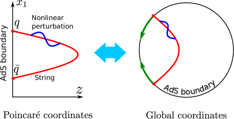
Figure 1: A dynamical string in Poincaré and global coordinates of AdS. Note that the string static in the Poincaré coordinates is mapped to a string with moving endpoints. We solve the time evolution of the perturbed string in the global coordinates and bring it back to the Poincaré coordinates.

In the rest of the paper, we begin with AdS coordinates in section 2, where we introduce a parametrization convenient for our numerical work. We then prepare for computing the string dynamics in the global AdS in section 3. We derive evolution equations, initial data, and boundary conditions. We also explain how to detect horizons of interest. In section 4, we show results for what we call longitudinal quenches. We first discuss a representative example and then investigate different quench parameters. In section 5, we show results for transverse quenches where the string moves in more space dimensions than the longitudinal ones. We close the paper with a summary and several discussions in section 6. Appendices contain technical details about numerical computations.

2 Anti-de Sitter spacetime in global and Poincaré coordinates

While our interest is on a string in the Poincaré coordinates of five-dimensional anti-de Sitter (AdS₅) spacetime, for convenience we make use of the global coordinates of AdS₅. For this reason, we start from comparing these coordinates.

AdS₅ is given by a hypersurface embedded in six-dimensional spacetime $R^{4,2}$. The metric of $R^{4,2}$ is

$$ds^{2}_{R^{4,2}}=-dX_{0}^{2}+dX_{1}^{2}+\cdots+dX_{4}^{2}-dX_{5}^{2}\ .$$ (1)

The embedding of AdS₅ is

$$-X_{0}^{2}-X_{5}^{2}+X_{1}^{2}+\cdots+X_{4}^{2}=-\ell^{2}\ .$$ (2)

where $\ell$ is a positive constant called the AdS radius.

The Poincaré coordinates cover only a part of the entire AdS spacetime. We specify the coordinates by $t,\,z,\,x_{i}$ ($i=1,2,3$). The Poincaré AdS₅ is given by

$$X_{0}=\frac{\ell\xi_{+}}{z}\ ,\quad X_{i}=\frac{\ell x_{i}}{z}\ ,\quad X_{4}=\frac{\ell\xi_{-}}{z}\ ,\quad X_{5}=\frac{\ell t}{z}\ ,$$ (3)

where we defined

$$\xi_{\pm}\equiv\frac{z^{2}+|\bm{x}|^{2}-t^{2}\pm\ell^{2}}{2\ell}\ .$$ (4)

The metric of the Poincaré AdS₅ is written as

$$ds^{2}=\frac{\ell^{2}}{z^{2}}(-dt^{2}+dz^{2}+d\bm{x}^{2})\ ,$$ (5)

The AdS radial coordinate $z$ takes $0<z<\infty$. The AdS boundary is at $z=0$, and the null surface $z=\infty$ is called Poincaré horizon. In these coordinates, the Poincaré horizon is at the coordinate singularity. The boundary of the Poincaré AdS is flat $1+3$ dimensional spacetime.

For our computations with strong perturbations, it is convenient to use the global coordinates which cover the entire AdS manifold beyond the Poincaré coordinates. In particular, we take Cartesian-like coordinates $\chi_{a}\ (a=1,2,3,4)$ where the spatial directions are conformally flat, and the global time is denoted by $\tau$. Such global coordinates are introduced by

$$\frac{X_{0}}{X_{5}}=\tan\tau\ ,\quad\frac{X_{a}}{\ell}=\frac{2\chi_{a}}{1-|\bm{\chi}|^{2}}\ ,$$ (6)

where $\bm{\chi}=(\chi_{1},\chi_{2},\chi_{3},\chi_{4})$ satisfies $|\bm{\chi}|\leq 1$. Note that both $\tau$ and $\bm{\chi}$ are dimensionless. The global AdS₅ metric is given by

$$ds^{2}=-\ell^{2}\left(\frac{1+|\bm{\chi}|^{2}}{1-|\bm{\chi}|^{2}}\right)^{2}d\tau^{2}+\frac{4\ell^{2}}{(1-|\bm{\chi}|^{2})^{2}}d\bm{\chi}^{2}.$$ (7)

The AdS boundary locates at $|\bm{\chi}|=1$ and has the topology of $S^{3}$. This metric is smooth at the AdS center $|\bm{\chi}|=0$. Although (6) implies the presence of a closed timelike curve, we can define $\tau$ in $-\infty<\tau<\infty$ by taking the universal covering.

From (3) and (6), we obtain the following coordinate transformation:

$$\begin{split}\tau&=\tan^{-1}(t/\xi_{+})+\begin{cases}\pi&(t>\xi_{0})\\ 0&(-\xi_{0}\leq t\leq\xi_{0})\\ -\pi&(t<-\xi_{0})\end{cases}\ ,\\ \chi_{i}&=\frac{x_{i}(\sqrt{\xi_{-}^{2}+z^{2}+|\bm{x}|^{2}}-z)}{\xi_{-}^{2}+|\bm{x}|^{2}}\quad(i=1,2,3)\ ,\\ \chi_{4}&=\frac{\xi_{-}(\sqrt{\xi_{-}^{2}+z^{2}+|\bm{x}|^{2}}-z)}{\xi_{-}^{2}+|\bm{x}|^{2}}\ ,\end{split}$$ (8)

where $\xi_{0}\equiv\sqrt{z^{2}+|\bm{x}|^{2}+\ell^{2}}$. In (8), one Poincaré patch is in $-\pi\leq\tau\leq\pi$. The inverse of (8) is given by

$$\frac{t}{\ell} =\frac{(1+|\bm{\chi}|^{2})\sin\tau}{(1+|\bm{\chi}|^{2})\cos\tau-2\chi_{4}}\ ,$$ (9)

$$\frac{z}{\ell} =\frac{1-|\bm{\chi}|^{2}}{(1+|\bm{\chi}|^{2})\cos\tau-2\chi_{4}}\ ,$$ (10)

$$\frac{x_{i}}{\ell} =\frac{2\chi_{i}}{(1+|\bm{\chi}|^{2})\cos\tau-2\chi_{4}}\quad(i=1,2,3)\ .$$ (11)

From (10), we find that the denominator must be zero at the the Poincaré horizon. The equation of the Poincaré horizon in the global coordinates hence becomes

$$\sum_{i=1}^{3}\chi_{i}^{2}+\left(\chi_{4}-\frac{1}{\cos\tau}\right)^{2}=\tan^{2}\tau\ .$$ (12)

This represents a $S^{3}$ with the center $(\chi_{i},\chi_{4})=(0,1/\cos\tau)$ and the radius $|\tan\tau|$. The Poincaré horizon is given by the cross section of this $S^{3}$ cut off by the unit $S^{3}$ of the AdS boundary $|\bm{\chi}|=1$. Moreover, if $x_{i}$ is finite on the Poincaré horizon, the numerator in (11) also has to be zero: $\chi_{i}=0$. Therefore, the part of the Poincare horizon at finite $x_{i}$ is mapped to a point given by $(\chi_{i},\chi_{4})=(0,(1-|\sin\tau|)/\cos\tau)$.

In Fig. 2, we show a schematic picture of AdS₅ spacetime in the global patch. When $\tau=\pm\pi$, the Poincaré patch shrinks to a point $(\chi_{i},\chi_{4})=(0,-1)$. Hence, the dynamics confined to a Poincaré patch becomes singular at that time, unless it jumps over the Poincare horizon before that time.

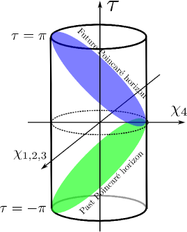
Figure 2: A schematic picture of AdS₅ spacetime. The inside of the cylinder is the global AdS₅ spacetime and its surface is the AdS boundary. Future and past Poincaré horizons are shown by inclined surfaces in the cylinder. The region surrounded by these surfaces corresponds to the Poincaré patch.

3 String dynamics in global AdS₅

We consider strong perturbations of the string in AdS₅. For this purpose, it is suitable to use the global coordinates (7) which is regular in the entire spacetime, rather than the Poincaré coordinates. Here, we describe the formulation to solve the string dynamics in the global AdS₅ numerically. We basically follow the method developed in Ishii:2014paa ; Ishii:2015wua .

3.1 Evolution equations

We make use of double null coordinates on the string worldsheet. When the worldsheet coordinates are denoted by $(u,v)$, the string in the target space is parametrized as

$$\tau=\tau(u,v)\ ,\quad\bm{\chi}=\bm{\chi}(u,v)\ .$$ (13)

Substituting them into Eq. (7), we obtain the components of the induced metric as

$$\gamma_{uu} =\frac{\ell^{2}}{(1-|\bm{\chi}|^{2})^{2}}\left(-(1+|\bm{\chi}|^{2})^{2}\,\tau_{,u}^{2}+4|\bm{\chi}_{,u}|^{2}\right)\ ,$$

$$\gamma_{vv} =\frac{\ell^{2}}{(1-|\bm{\chi}|^{2})^{2}}\left(-(1+|\bm{\chi}|^{2})^{2}\,\tau_{,v}^{2}+4|\bm{\chi}_{,u}|^{2}\right)\ ,$$

$$\gamma_{uv} =\frac{\ell^{2}}{(1-|\bm{\chi}|^{2})^{2}}\left(-(1+|\bm{\chi}|^{2})^{2}\,\tau_{,u}\tau_{,v}+4\bm{\chi}_{,u}\cdot\bm{\chi}_{,v}\right)\ ,$$ (14)

Using the reparametrization freedom of the worldsheet coordinates, we impose the double null condition on the induced metric as

$$C_{1}\equiv\gamma_{uu}=0\ ,\qquad C_{2}\equiv\gamma_{vv}=0\ .$$ (15)

From the double null conditions, we obtain

$$\tau_{,u}=\frac{2|\bm{\chi}_{,u}|}{1+|\bm{\chi}|^{2}}\ ,\quad\tau_{,v}=\frac{2|\bm{\chi}_{,v}|}{1+|\bm{\chi}|^{2}}\ ,$$ (16)

where we took the positive signature regarding $\partial_{u}$ and $\partial_{v}$ as future directed null vectors. In the double null coordinates, the Nambu-Goto action is written as

$$\begin{split}S&=-\frac{1}{2\pi\alpha^{\prime}}\int dudv\sqrt{\gamma_{uv}^{2}-\gamma_{uu}\gamma_{vv}}=\frac{1}{2\pi\alpha^{\prime}}\int dudv\gamma_{uv}\\ &=\frac{\sqrt{\lambda}}{2\pi}\int dudv\,\frac{1}{(1-|\bm{\chi}|^{2})^{2}}\left(-(1+|\bm{\chi}|^{2})^{2}\,\tau_{,u}\tau_{,v}+4\bm{\chi}_{,u}\cdot\bm{\chi}_{,v}\right)\ ,\end{split}$$ (17)

where in the second equality we used the double null conditions (15) and $\gamma_{uv}<0$. The ’t Hooft coupling is defined by $\lambda\equiv\ell^{4}/\alpha^{\prime}{}^{2}$. The string evolution equations are given by

$$\tau_{,uv}=-\frac{8}{(1-|\bm{\chi}|^{2})(1+|\bm{\chi}|^{2})^{2}}\left(|\bm{\chi}_{,u}|\bm{\chi}_{,v}+\bm{\chi}_{,u}|\bm{\chi}_{,v}|\right)\cdot\bm{\chi}\ ,$$

$$\bm{\chi}_{,uv}=-\frac{2}{1-|\bm{\chi}|^{4}}\Big{[}2|\bm{\chi}_{,u}||\bm{\chi}_{,v}|\bm{\chi}$$

$$\hskip 64.58313pt+(1+|\bm{\chi}|^{2})\big{\{}(\bm{\chi}\cdot\bm{\chi}_{,v})\bm{\chi}_{,u}+(\bm{\chi}\cdot\bm{\chi}_{,u})\bm{\chi}_{,v}-(\bm{\chi}_{,u}\cdot\bm{\chi}_{,v})\bm{\chi}\big{\}}\Big{]}\ ,$$ (18)

where in the right hand sides, we eliminated $\tau_{,u}$ and $\tau_{,v}$ by using Eq. (16). This process is very important for stabilizing numerical calculations.

3.2 Poincaré static string in the global patch

As the initial configuration, we consider a static string hanging in the Poincaré AdS from the boundary. Its endpoints correspond to a pair of quark and antiquark. We locate the endpoints at $x_{1}=\pm L/2$ and $x_{2}=x_{3}=0$ where $L$ is the separation. We call the one with $x_{1}=L/2$ the quark endpoint. The static solution parametrized by the double null coordinates $(u,v)$ was obtained in Ishii:2015wua as

$$t=z_{0}\,(u+v)\ ,\quad z=z_{0}\,f(u-v)\ ,\quad x_{1}=z_{0}\,g(u-v)\ ,\quad x_{2}=x_{3}=0\ ,$$ (19)

where $z_{0}\equiv L/(2\Gamma_{0})$ and $\Gamma_{0}\equiv\sqrt{2}\pi^{3/2}/\Gamma(1/4)^{2}\simeq 0.599$. The constant $z_{0}$ represents the maximum value of the $z$-coordinate that the string reaches. The functions $f$ and $g$ are defined as

$$f(\phi)\equiv\textrm{sn}(\phi;i)\ ,\quad g(\phi)\equiv-\int^{\phi}_{\beta_{0}/2}d\phi^{\prime}\,f(\phi^{\prime})^{2}\ ,$$ (20)

where $\textrm{sn}(x;k)$ is the Jacobi elliptic function. The constant $\beta_{0}\equiv\pi/(2\Gamma_{0})\simeq 2.622$ is the minimum positive root of $\textrm{sn}(x;i)$, and in (19) we have used the worldsheet reparametrization degrees of freedom to locate the two boundaries of the open string worldsheet at $u=v$ and $u=v+\beta_{0}$.

We map the Poincaré patch’s static solution (19) to the global coordinates. This is done by substituting it into Eq. (8). It is straightforward to check that the mapped solution satisfy the evolution equations (18) and the constraints (15). The solution static in the Poincaré patch (19) becomes a $\tau$-dependent solution in the global coordinates. In Fig. 3, we show the string configurations for several $\tau$-slices. Note that $\chi_{2}=\chi_{3}=0$ for the static solution, and hence Fig. 3 corresponds to the spatial part of an AdS₃ slice in the AdS₅. The string shrinks as $\tau$ approaches $\pi$ as the Poincaré horizon surrounding the string also does. Eventually, both the static string and the Poincaré horizon collapse to a point at $\tau=\pi$. The string configurations are symmetric under $\tau\to-\tau$, and thus the string expands as $\tau$ increases for $-\pi\leq\tau\leq 0$.

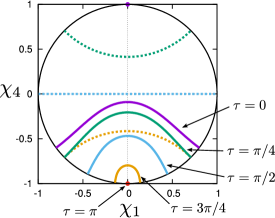
Figure 3: Mapping of the Poincaré static hanging string to the global coordinates when $\ell/L=1$. The colored lines correspond to the string configurations when $\tau=0,\,\pi/4,\,\pi/2,\,3\pi/4$ from the top, and the red dot at $(\chi_{1},\chi_{4})=(0,-1)$ is that for $\tau=\pi$. The three dashed lines as well as the dots at $(\chi_{1},\chi_{4})=(0,\pm 1)$ are the Poincare horizon at each corresponding time. Their ordering from the top is the same as that of the string.

In the Poincaré coordinates, the AdS radius $\ell$ does not appear in the equations and solution of the string. However, the transformation (8) involves $\ell$, and therefore the string configurations in the global coordinates look differently depending on $\ell/L$. For instance, Fig. 3 is drawn when $\ell/L=1$. Nevertheless, once the string dynamics computed in the global coordinates is transformed back to the Poincaré patch, the dependence on $\ell$ disappears. We can hence use arbitrary values of $\ell/L$ convenient for numerical computations.

For the time evolution, we take $v=0$ as the initial surface and use the Poincaré static solution mapped to the global coordinates as the initial data. Nontrivial string dynamics is induced by changing the boundary conditions at the string endpoints in time.

3.3 Boundary conditions

In the Poincaré patch, the two string endpoints are denoted by $\bm{x}=\bm{x}_{q}(t)$ and $\bm{x}_{\bar{q}}(t)$, corresponding to the locations of the quark and antiquark, respectively. We induce dynamics on the string by changing their positions. Since we are interested in the dynamics in the Poincaré patch, we specify the patterns of endpoint motion as functions there. In solving the time evolution in the global patch, the quark positions are translated to the global coordinates’ boundary through Eq. (8).

To introduce perturbations on the string, we move the quark endpoint for a time duration $\Delta t$ with amplitude $\epsilon$. In particular, we consider the following three kinds of “quenches”:

1. Longitudinal quench:

   $$\bm{x}_{q}(t)=\left(\frac{L}{2}+\epsilon L\alpha(t),0,0\right)\ .$$ (21)

2. Transverse linear quench:

   $$\bm{x}_{q}(t)=\left(\frac{L}{2},\epsilon L\alpha(t),0\right)\ .$$ (22)

3. Transverse circular quench:

   $$\bm{x}_{q}(t)=\left(\frac{L}{2},\epsilon L\alpha(t),\pm\epsilon L\sqrt{\alpha(t)(1-\alpha(t))}\right)\ ,$$ (23)

   where the upper and lower signs are taken for $t\leq\Delta t/2$ and $t>\Delta t/2$, respectively.

The other endpoint is fixed at the original position: $\bm{x}_{\bar{q}}(t)=(-L/2,0,0)$. The function $\alpha(t)$ is a compactly supported $C^{\infty}$ function defined by

$$\alpha(t)=\begin{cases}\exp\left[2\left(\frac{\Delta t}{t-\Delta t}-\frac{\Delta t}{t}+4\right)\right]\qquad&(0<t<\Delta t)\\ 0\qquad&(\textrm{else})\end{cases}\ .$$ (24)

This function has the maximum value $1$ at $t=\Delta t/2$. In Fig. 4, we show schematic pictures of the quenches (i)-(iii). For later convenience, we introduce the velocity and the Lorentz factor of the quark as

$$\bm{v}(t)\equiv\frac{d\bm{x}_{q}(t)}{dt}\ ,\quad\gamma(t)\equiv\frac{1}{\sqrt{1-\bm{v}^{2}(t)}}\ .$$ (25)

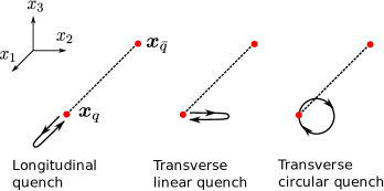
Figure 4: Schematic pictures of the quenches.

These quench patterns are the same as those considered in Ishii:2015wua and chosen to represent typical string motions, particularly with different dimensionality. For quenches (i) and (ii), the motion of the string is restricted in (2+1)- and (3+1)-dimensions, respectively. On the other hand, by the quench (iii), fluctuations along both $x_{2}$- and $x_{3}$-directions are induced, and the string moves in all (4+1)-dimensions. The significant difference from Ishii:2015wua in this paper is the magnitude of $\epsilon$, which we choose much bigger.

Using the residual coordinate freedoms $u=u(\bar{u})$ and $v=v(\bar{v})$, we fix the locations of the string endpoints on the worldsheet to $u=v$ and $u=v+\beta_{0}$. Letting $\bm{\chi}_{q}(\tau)$ and $\bm{\chi}_{\bar{q}}(\tau)$ denote the trajectories of the endpoints in the global patch, we write the boundary conditions for $\bm{\chi}(u,v)$ as

$$\bm{\chi}|_{u=v}=\bm{\chi}_{q}(\tau)\ ,\quad\bm{\chi}|_{u=v+\beta_{0}}=\bm{\chi}_{\bar{q}}(\tau)\ .$$ (26)

The functional form of $\bm{\chi}(\tau)$ is found from $(\tau,\bm{\chi})$ through (8) where the right hand sides are determined by the quark and antiquark positions in the Poincaré patch’s boundary. While the endpoints are quenched, it is hard to find analytic expressions of $\bm{\chi}(\tau)$. It is practical to find the relation between $\tau$ and $\bm{\chi}$ numerically at each time.

Outside the quench period, however, simple expressions for (26) can be obtained. When $\bm{x}=(\tilde{x},0,0)$ is constant, we can eliminate $t$ and $z$ from (8) and obtain

$$\begin{split}\chi_{1}|_{\mathrm{bdry}}&=\frac{\ell\tilde{x}\cos\tau+\tilde{x}\sqrt{\tilde{x}^{2}\sin^{2}\!\tau+\ell^{2}}}{\tilde{x}^{2}+\ell^{2}}\ ,\\ \chi_{4}|_{\mathrm{bdry}}&=\frac{\tilde{x}^{2}\cos\tau-\ell\sqrt{\tilde{x}^{2}\sin^{2}\!\tau+\ell^{2}}}{\tilde{x}^{2}+\ell^{2}}\ ,\end{split}$$ (27)

with $\chi_{2}=\chi_{3}=0$. In our case, $\tilde{x}=\pm L/2$.

At the boundaries, we evolve $\tau(u,v)$ by satisfying the boundary conditions (26). At $|\bm{\chi}|=1$, the constraint equations (16) reduce to

$$\tau_{,u}=|\bm{\chi}_{,u}|\ ,\quad\tau_{,v}=|\bm{\chi}_{,v}|\ .$$ (28)

Solving these equations, we determine the consistent evolution of $(\tau,\bm{\chi})$.

To solve the time evolution, we use the numerical method explained in Ishii:2015wua . (See its Appendix A for details.) We introduce a grid with spacing $\Delta u=\Delta v=h$ on the $(u,v)$-coordinates and then discretize the equations of motion with second-order finite differentials. How to discretize the boundary evolution (28) for this global AdS case is described in Appendix A. In Appendix B, numerical errors are evaluated.

3.4 String dynamics and horizons

Solving the evolution equations (18), we obtain $\tau(u,v)$ and $\bm{\chi}(u,v)$ as functions on the worldsheet. We compare the solution with horizons relevant to our string dynamics.

Poincaré horizon

One of this paper’s interests is to see whether the string can reach the Poincaré horizon. In the global coordinates, the target space metric is regular at the Poincaré horizon. Hence there is no obligation for the dynamical string to cross the surface. To check if this occurs, we compare the solution with (12). On the worldsheet, the locations crossing the Poincaré horizon, if exist, are continuous and form a spacelike curve connecting the two boundary points with $\tau=\pi$.

Whether the Poincaré horizon is crossed or not also divides the fate of the string evolution. If the string does not cross the horizon, it shrinks to one point $(\chi_{1},\chi_{2},\chi_{3},\chi_{4})=(0,0,0,-1)$ at $\tau=\pi$. On the worldsheet point of view, the fields $\tau(u,v)$ and $\bm{\chi}(u,v)$ converge to the limiting values as $(u,v)\to\infty$. However, at $\tau=\pi$, denominators in the right hand sides of the evolution equations (18) become close to zero, and numerical calculations break down as $\tau=\pi$ is approached. This fate is different if the string cross the Poincaré horizon by strong quenches. In this case, the string extends in the global AdS at $\tau=\pi$. Then (18) is regular, and the numerical calculations can continue to $\tau>\pi$. In Fig. 5, we show the string worldsheet for such a case schematically.

Worldsheet effective horizons

The part of the string worldsheet that have crossed the Poincaré horizon, of course, is not visible from the boundary in a Poincaré patch. Before the Poincaré horizon, the string worldsheet has dynamically created effective horizons from the inside of which no signal reaches the AdS boundary in the Poincaré patch. We can define the effective horizons as the boundary of the causal past of the string endpoints at $\tau=\pi$. In Fig. 5, the effective horizons are drawn with blue and red lines, which are respectively at constant $v$ and $u$. We also drew the Poincaré horizon with a black dashed curve. The Poincaré horizon is hidden in the effective horizons. Once the string plunges into the Poincaré horizon, the quark and antiquark are disconnected informationally in the Poincaré patch. For this reason, we will sometimes refer to the plunge of the string into the Poincaré horizon as the disconnection of the string

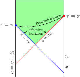
Figure 5: Poincaré and effective horizons on the worldsheet.

Practically, we can identify the effective horizons in the numerical solutions as follows. We monitor $\tau(u,v)$ at each boundary and find $u=u_{H}$ and $v=v_{H}$ such that $\tau(u_{H},u_{H})=\pi$ and $\tau(v_{H}+\beta_{0},v_{H})=\pi$, respectively. (These are shown by red and blue points in Fig. 5.) Then, the effective horizon is given by $\mathcal{H}=\{(u,v)|u=u_{H},v\geq v_{H}\}\bigcup\{(u,v)|v=v_{H},u\geq u_{H}\}$. This specify the region that cannot be seen from both endpoints. This part is shaded with green in Fig. 5. Note that each of the triangular region surrounded by the dashed and solid lines and a boundary can be seen only from one endpoint.

4 Longitudinal quench

We show results of string dynamics. We start from the longitudinal quench (21), which exhibits typical phenomena. We will also discuss the transverse quenches (22) and (23) in the following section, emphasizing similarities and differences.

4.1 String dynamics

As a representative example, we consider the longitudinal quench with $\epsilon=0.15$ and $\Delta t/L=2$. In Fig. 6, we show snapshots of the string in the global patch for $\ell/L=1$. Starting from a static hanging string configuration at $\tau=0$, we observe that a wave is induced on the string by the quench ($\tau=\pi/2$). As $\tau=\pi$ approaches, we find that the string extends beyond the Poincaré horizon ($\tau=7\pi/8$), and when $\tau=\pi$ the string keeps a finite length, in contrast to the shrinking static string in Fig. 3 (and strings with small perturbations as well). We thus find that this parameter choice corresponds to a case where the dynamical string crosses the Poincaré horizon.

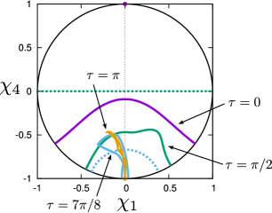
Figure 6: Snapshots of the string dynamics in the global patch for the longitudinal quench with $\epsilon=0.15$ and $\Delta t/L=2$ for $\ell/L=1$. The real lines correspond to the string, and the dashed lines the Poincaré horizon.

We look into this dynamical string in Fig. 7. In these plots, thick and thin curves correspond to the string configurations and Poincaré horizons, respectively, and the part of the string inside of the worldsheet effective event horizons is depicted by the dashed curves. Note that for variables in the global coordinates nothing irregular happens. For $2\leq\tau\leq 2.3$, we see that the string is smooth and does not reach the Poincaré horizon. At $\tau\geq 2.4$, cusps and self-intersection appear on the string. We then observe that the string crosses the Poincaré horizon around $\tau\simeq 2.6$. Prior to this time, the pair of the effective horizons appears around $\tau\simeq 2.1$.

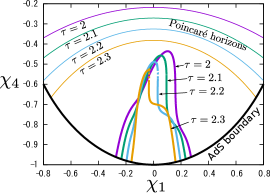
(a) $2\leq\tau\leq 2.3$

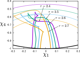
(b) $2.4\leq\tau\leq 2.7$

Figure 7: More snapshots of the string dynamics in the global patch for the longitudinal quench with $\epsilon=0.15$ and $\Delta t/L=2$ for $\ell/L=1$. Figs. (a) and (b) are for $2\leq\tau\leq 2.3$ and $2.4\leq\tau\leq 2.7$, respectively. The thick and thin curves correspond to the string configurations and Poincaré horizons. The part of the string depicted by the dashed curve is inside of the effective event horizons on the worldsheet.

This string motion in the global patch is seen as disconnection of the string in the Poincaré patch. The numerical solutions $\tau(u,v)$ and $\bm{\chi}(u,v)$ are mapped to the Poincaré patch’s $t=T(u,v)$, $z=Z(u,v)$ and $\bm{x}=\bm{X}(u,v)$ through Eqs. (9-11). In Fig. 8, we show the corresponding string dynamics in the Poincaré patch. The string becomes longer as $t$ increases, and in the late time its configuration eventually approaches two straight strings. We find that the effective event horizons appear around $t/L\simeq 2.54$.

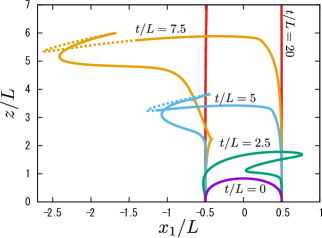
Figure 8: Snapshots of the string dynamics in the Poincaré patch for the longitudinal quench with $\epsilon=0.15$ and $\Delta t/L=2$. The effective horizons appear on the worldsheet within finite time. The string configuration approaches two straight strings in the late time.

While our time evolution is for purely classical strings, physically finite-$N_{c}$ effects can be important at the cusps and self-intersection points. This implies that time evolution after their appearance may significantly alter due to such corrections, if they are formed before the event horizons. However, as we will see in section 5, in more general cases involving string dynamics in all $(4+1)$-dimensions, no cusp formation nor self-intersection is found. Hence practically it is not likely that the dynamical disconnection are prevented by the finite-$N_{c}$ effects in general quenches.

4.2 Forces acting on the quarks

Forces act on the quark and antiquark endpoints as the response of the string. In view of the gauge/gravity duality, the position of the string endpoint corresponds to the “source” of the field theory operator dual to the string, and that operator is the force. We compute the forces in the Poincaré patch, after the dynamical string solution is mapped from the global coordinates. Let $x_{i}=X_{i}(t,z)$ denote the string coordinates in the target space. The force on the quark is then given by Ishii:2015wua

$$F_{i}(t)=\frac{\sqrt{\lambda}}{4\pi}\gamma^{-1}(\delta_{ij}+\gamma^{2}v_{i}v_{j})\partial_{z}^{3}X_{j}(t,z)|_{z=0,\bm{x}=\bm{x}_{q}}\ .$$ (29)

where the velocity $\bm{v}$ and Lorentz factor $\gamma$ have been defined in Eq. (25). The force on the antiquark can be simply given by changing $\bm{x}_{q}\to\bm{x}_{\bar{q}}$ with $\bm{v}=0$ and $\gamma=1$.

In Fig. 9, the absolute values of the forces for the longitudinal quench with $\epsilon=0.15$ and $\Delta t/L=2$ is shown in a log-log scale. In the plots, the forces on the quark and antiquark are denoted by $\bm{F}$ and $\bar{\bm{F}}$. As $t\to\infty$, both $\bm{F}$ and $\bar{\bm{F}}$ approach zero. This also indicates that the flux tube disconnects, and the final configuration (in $t\to\infty$) is two straight strings. The divergence in $\bar{\bm{F}}$ at $t/L\sim 10$ is due to a cusp arriving at the boundary. (See Ishii:2015wua .) Once the cusp passes, $\bar{\bm{F}}$ monotonically decays and its behavior seems to approach that of $\bm{F}$.

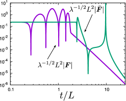
Figure 9: The forces acting on the quark and antiquark for the longitudinal quench with $\epsilon=0.15$ and $\Delta t/L=2$.

In the late time behavior of the forces, we observe power law decay. This is clearly seen in $\bm{F}$. In the case of $\epsilon=0.15$ and $\Delta t/L=2$, a fit of the power law in $\bm{F}$ is $t^{-n}$ with $n\sim 3.8$. It appears that $\bar{\bm{F}}$ also realizes power law decay, but because of its different evolution from $\bm{F}$ such as the travel of the cusp, the approach of $\bar{\bm{F}}$ to a power law seems quite delayed.

The power depends on the quench parameters. In Fig. 10, we compare $\bm{F}$ for $\epsilon=$0.1, 0.125, 0.15 when $\Delta t/L=2$. With the first value, the string extends its length a little but does not reach the Poincaré horizon, and the late time oscillations in the plot is due to bounces of cusps Ishii:2015wua . For the latter two, the string reaches the Poincaré horizon. As seen in the $\epsilon=0.1$ plot, the power law can be observed even when the string does not reach the horizon, although it is disturbed by the travel of waves and cusps on the string. The power law exponent is read off $n\sim$ 2, 3.3, 3.8 for $\epsilon=$0.1, 0.125, 0.15, respectively. The decay becomes steeper as $\epsilon$ increases. The dependence on the quench parameters implies that the slope of the power law is not simply fixed by the AdS background.

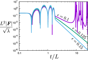
Figure 10: Comparison of the forces acting on the quark for $\epsilon=$0.1, 0.125 and 0.15 when $\Delta t/L=2$.

What is the origin of the power law tail? One of the most plausible explanations for the power law tail can be given by the redshift of the effective horizon. Before going to detailed arguments, we emphasize that the curved initial configuration of the string is also important. Let us define “left moving” as “from the quark to antiquark” ($\bm{x}_{q}\to\bm{x}_{\bar{q}}$) and “right moving” as “from the antiquark to quark” ($\bm{x}_{\bar{q}}\to\bm{x}_{q}$). While a left moving wave is mainly generated on the worldsheet by the quench, right moving waves are also generated secondarily from the backscattering by the curvature of the hanging-shape string and/or the reflection at the other boundary. Such right moving waves then can propagate back to the quark endpoint. Later in this section, we will discuss that starting from a straight string and adding boundary quenches do not result in producing a power law.

Suppose that the left and right moving waves are present on the string and effective event horizons are formed on the string. We then focus on the force on the quark endpoint. Let us consider a right moving wave which has a non-trivial profile at the effective horizon. A wave from near the horizon needs very long time to reach the AdS boundary and would cause the tail in the force. For an asymptotically AdS black hole with finite surface gravity $\kappa$, perturbations decay with $\sim e^{-\kappa t}$. In the present case, however, the effective horizon approaches the Poincaré horizon that can be regarded as an extremal horizon ($\kappa=0$). For an extremal case, the exponential decay is absent and replaced by a power law decay Aretakis:2011ha ; Aretakis:2011hc ; Lucietti:2012xr ; Murata:2013daa . The worldsheet effective horizons on the string in pure AdS might inherit such a property.

The presence of the power law decay of a perturbation can be demonstrated by a linear theory as follows. (See also Lucietti:2012xr for the explicit calculation of the propagation of a scalar field in AdS₂.) Let us consider a perturbation around a trivial solution of a straight string: $\bm{X}(t,z)=0$. The equation for the linearized perturbation is simply given by

$$\left(\partial_{t}^{2}-\partial_{z}^{2}+\frac{2}{z}\partial_{z}\right)\delta X_{1}(t,z)=0\ ,$$ (30)

where we consider the perturbation only along the $x_{1}$-direction. Its general solution is given by

$$\delta X_{1}(t,z)=f_{L}(t-z)-f_{R}(t+z)+z\{\dot{f}_{L}(t-z)+\dot{f}_{R}(t+z)\}\ ,$$ (31)

where $f_{L}$ and $f_{R}$ are arbitrary functions which represent left and right moving waves. If we put a compactly supported initial data as usually done in perturbation theory analyses, we can never observe a power law tail. However, as seen in Fig. 8, the string is bent even at the effective horizon in our numerical calculations. For this reason, as a toy model that has non-trivial profile near the horizon, we consider initial data, $\delta X_{1}|_{t=0}\sim 1/z^{n}$ $(z\to\infty)$ and $\delta\dot{X}_{1}|_{t=0}=0$, where $n$ is a non-negative constant. We also impose Dirichlet boundary condition at $z=0$. Then, the arbitrary functions are determined as $f_{R}(x)=f_{L}(x)\sim 1/x^{n}$ $(x\to\infty)$. Substituting them into Eq. (31) and taking the limit of $t\to\infty$ for a fixed $z$, we obtain $\delta X_{1}\sim z^{3}/t^{n+3}$. Therefore, the force on the quark could obey a power law as $F\propto\partial_{z}^{3}\delta X_{1}|_{z=0}\sim 1/t^{n+3}$. Of course, in our actual numerical calculations, the profile of the string after the quench is not so simple as $\delta X_{1}|_{t=0}\sim 1/z^{n}$ but depends on details of how the string is deformed by the quenches. That would cause $\epsilon$ and $\Delta t$ dependence of the power law exponent. In particular, in our nonlinear numerical results $F\propto 1/t^{n}$ with $n<3$ is possible, which cannot be explained by the assumption in this paragraph’s linear theory arguments.

As seen in Fig. 10, the power law decay is temporarily present even for $\epsilon=0.1$ and $\Delta t/L=2$ with which the string does not plunge into the Poincaré horizon. This behavior can be observed roughly until the string stops expanding. It would be fair to speculate that redshift effects on the stretching string might be generally responsible for causing the power law even if worldsheet event horizons are not formed.

The power law tail would be regarded as a relic of the dynamical “phase transition” between the hanging string and two straight strings. That is, the initial curved configuration of the string producing “right-moving” waves might be important. Actually, we can never observe the power law tail if we perturb the endpoint of the straight string (single quark). Let us consider a linear perturbation again. Imposing the boundary condition $\delta X_{1}|_{z=0}=x_{q}(t)$ and the initial condition $\delta X_{1}|_{t=0}=\delta\dot{X}_{1}|_{t=0}=0$, we obtain a solution as $\delta X_{1}=x_{q}(t-z)+z\dot{x}_{q}(t-z)$. This solution is purely ingoing wave and there is no backscattering. After the quench, therefore, the force on the quark becomes exactly zero and cannot have a power law tail. Although here we considered the linear perturbation for simplicity, the same consequence can be shown even for the full nonlinear solution obtained in Mikhailov:2003er , which applies to the Poincaré straight string. We also computed nonlinear evolution of a straight string with boundary perturbations by using our numerical methods and checked that the force dropped to zero without a tail.

4.3 Condition for the disconnection

Stepping forward from the above example, we investigate dependence on the quench parameters. On one hand, we compute the energy of the dynamical string and evaluate the energy increase by quenches. On the other hand, we directly search critical parameters for the string to cross the Poincaré horizon. By comparing the results, we argue the condition for the string disconnection.

Let us derive the formula for evaluating the energy of the dynamical string. In the global patch, the worldsheet action is given by (17). Using Eq. (8), we can rewrite the action in terms of the Poincaré coordinates as

$$\begin{split}S&=\frac{\sqrt{\lambda}}{2\pi}\int dudv\,\frac{1}{Z^{2}}(-T_{,u}T_{,v}+Z_{,u}Z_{,v}+\bm{X}_{,u}\cdot\bm{X}_{,v})\\ &=\frac{\sqrt{\lambda}}{4\pi}\int d\sigma^{0}d\sigma^{1}\,\frac{1}{Z^{2}}\eta^{ab}(T_{,a}T_{,b}-Z_{,a}Z_{,b}-\bm{X}_{,a}\cdot\bm{X}_{,b})\ ,\end{split}$$ (32)

where we introduced $\sigma^{0}=u+v$, $\sigma^{1}=u-v$, and $\eta^{ab}=\textrm{diag}(-1,1)$. The domains of the coordinates are $-\infty<\sigma^{0}<\infty$ and $0\leq\sigma^{1}\leq\beta_{0}$. This action is invariant under the time translation: $T\to T+\textrm{const}$. Its conserved current is given by

$$P^{a}=\frac{\sqrt{\lambda}}{2\pi}\frac{1}{Z^{2}}\eta^{ab}T_{,b}\ .$$ (33)

To compute the string total energy, we integrate $P^{0}$ along $\sigma_{1}$ for fixed $\sigma_{0}$,

$$E_{\textrm{bare}}=-\int d\sigma^{1}P^{0}=\frac{\sqrt{\lambda}}{2\pi}\int_{\epsilon}^{\beta_{0}-\epsilon^{\prime}}d\sigma^{1}\,\frac{\partial_{0}T}{Z^{2}}\ .$$ (34)

This quantity diverges in the limits of $\epsilon\to 0$ and $\epsilon^{\prime}\to 0$ due to contributions at the AdS boundary. The divergence is interpreted as coming from the energy of the infinitely heavy quarks $\sim m_{q}\gamma$ and $m_{\bar{q}}\bar{\gamma}$. The energy is regularized by adding counter terms as

$$\begin{split}E_{\textrm{reg}}&=E_{\textrm{bare}}-\frac{\sqrt{\lambda}}{2\pi}\left[\left.\frac{\gamma(T)}{Z}\right|_{\sigma^{1}=\epsilon}+\left.\frac{\bar{\gamma}(T)}{Z}\right|_{\sigma^{1}=\beta_{0}-\epsilon^{\prime}}\right]\ .\end{split}$$ (35)

Substituting the static hanging string solution (19) into the above expression, we obtain the static energy as $E_{\mathrm{stat}}L/\sqrt{\lambda}=-4\pi^{2}/\Gamma(1/4)^{4}\simeq-0.2285$, consistent with the result in Rey:1998ik ; Maldacena:1998im . This value corresponds to the energy difference between the static hanging string and straight strings, where the regularized energy of the latter is zero.

In actual numerical calculations, we include the boundary terms in the integrand as

$$E_{\textrm{reg}}=\frac{\sqrt{\lambda}}{2\pi}\int^{\beta_{0}}_{0}d\sigma^{1}\,\left[\frac{\partial_{0}T}{Z^{2}}-\partial_{1}\left(\frac{s(\sigma^{1})}{Z}\right)\right]\ ,$$ (36)

where $s(\sigma^{1})$ is any smooth function satisfying $s=\gamma(T)|_{\sigma^{1}=0}+\mathcal{O}((\sigma^{1})^{2})$ ($\sigma^{1}\to 0$) and $s=-\bar{\gamma}(T)|_{\sigma^{1}=\beta_{0}}+\mathcal{O}((\beta_{0}-\sigma^{1})^{2})$ ($\sigma^{1}\to\beta_{0}$). This form is convenient because the integrand is finite at $\sigma^{1}=0$ and $\beta_{0}$. The difference between the time dependent value of (36) and the static value gives the amount of energy injected to the string by the quench until that moment. Evaluating the energy increase in $t\geq\Delta t$ gives the total addition of the energy.

By changing $\epsilon$ and $\Delta t$, we compute the energies injected to the string. In particular, we are interested in quenches where the total energy injection is equal to the energy difference between the straight and hanging strings. We obtain the values of $(\epsilon,\Delta t)$ for such critical injections. The results will be soon discussed in Fig. 11.

An alternative way to evaluate the amount of the energy injection is to compute the work done on the quark endpoints. The total work is given by

$$W=-\int_{C}d\bm{x}\cdot\bm{F}=-\int_{0}^{\Delta t}dt\,\bm{v}\cdot\bm{F}\ ,$$ (37)

where in the last expression we used the fact that our quench patterns are compact in time. The integrand $\bm{v}\cdot\bm{F}$ has the form of the product of time derivative of the “source” and the “response” in the sense of holography and reflects non-conservation of the energy in the presence of a time dependent source. We checked that the total work computed by evaluating (37) agrees with the energy change evaluated from (36).

We also directly search for critical quench parameters for the string to cross the Poincaré horizon. For a fixed $\Delta t$, we start from a large amplitude and measure $\tau$ when the string crosses the horizon. As the amplitude is decreased, the crossing time approaches $\tau=\pi$, but computations also become difficult around $\chi_{4}=-1$. While we can compute for crossing times very close to $\tau=\pi$, once numerical errors become significant, we use an extrapolation to estimate the critical amplitude with which the crossing time would be $\tau=\pi$. We repeat this by changing $\Delta t$ and obtain critical $(\epsilon,\Delta t/L)$

In Fig. 11, we plot the results of the searches. The result of the energy injection equal to the difference between the two string configurations (i.e. when Eq. (36) gives $E_{\textrm{reg}}=0$) is plotted with a line. That from the direct search for the horizon crossing is plotted with dots. Remarkably, these two results agree. This implies that if the amount of the energy larger than the static energy is injected, the hanging string dynamically changes its topology to two straight strings. By this process, the two endpoints are causally disconnected. This phenomenon is seen in the dual field theory as a breaking of the flux tube when the energy bigger than the “binding” energy is supplied.

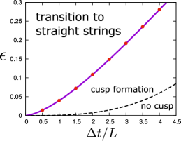
Figure 11: Results of the evaluation of the string configuration change in $(\epsilon,\Delta t/L)$-parameters. The dots are the critical parameters obtained from the direct search. The real line corresponds to the energy injection equal to the energy difference of the two static string configurations. For comparison, an estimation of the threshold for cusp formation $\epsilon=9.3\times 10^{-4}(\Delta t/L)^{3}$ obtained in Ishii:2015wua is also plotted with the dashed line.

We can show that the string cannot plunge into the Poincaré horizon for $E_{\textrm{reg}}<0$ as follows. Let us consider dynamical solutions intersecting with the Poincaré horizon. In terms of Poincaré target space coordinates, the regularized energy for such a string is given by

$$E_{\textrm{reg}}=\frac{\sqrt{\lambda}}{2\pi}\int^{\infty}_{0}dz\left[\frac{1+\bm{X}^{\prime}{}^{2}}{z^{2}\sqrt{(1-\dot{\bm{X}}^{2})(1+\bm{X}^{\prime}{}^{2})-(\dot{\bm{X}}\cdot\bm{X}^{\prime})^{2}}}-\frac{1}{z^{2}}\right]\ ,$$ (38)

where we took the upper bound of the integration as $z=\infty$ since the string intersects with the horizon, and $\dot{\bm{X}}\equiv\partial_{t}\bm{X}$ and $\bm{X}^{\prime}\equiv\partial_{z}\bm{X}$. It is straightforward to check that the straight static string $\bm{X}(t,z)=0$ minimizes the above energy as $E_{\textrm{reg}}=0$. This implies that, even if time-dependence is taken into account, string configurations with $E_{\textrm{reg}}<0$ cannot intersect with the horizon.

Does a string with $E_{\textrm{reg}}>0$ always intersect with the Poincaré horizon? This is a difficult question since to obtain an answer it is necessary to consider all time dependent solutions with positive energies. At least in our numerical calculations, the final fate of the string dynamics for $E_{\textrm{reg}}>0$ was always straight strings. The straight strings may be regarded as an attractor for positive energy solutions. It would be interesting to see if it is possible to find fine-tuned initial data and boundary conditions by which a string never plunges into the horizon.

5 Transverse quenches

We also consider transverse quenches where string motions are in more spatial dimensions than the longitudinal quenches. In Fig. 12, we show snapshots of the string dynamics for the transverse linear quench (22) with $\epsilon=0.2$ and $\Delta t/L=2$. The string motion is in the ($3+1$)-dimensions spanned by ($t,\chi_{1},\chi_{2},\chi_{4}$). Fig. 12(a) visualizes that the string plunges into the Poincaré horizon accompanied by the effective horizon formation on the worldsheet. The solution mapped to the Poincaré patch is shown in Fig. 12(b). The string becomes longer as $t$ increases and in the late time approaches the configuration with two straight strings. Although it is not so much clear in Fig. 12, we found cusp formation by checking roots of the Jacobian $\tau_{,u}\bm{\chi}_{,v}-\tau_{,v}\bm{\chi}_{,u}$ Ishii:2015wua . On the other hand, we did not observe self-intersections of the string in this example although it is possible from the dimensional point of view for the transverse linear quench. Self intersections of the string could be observed in general ($3+1$)-dimensional string dynamics.

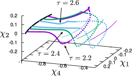
(a) Global patch

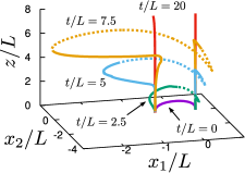
(b) Poincaré patch

Figure 12: Snapshots of the string dynamics for the transverse linear quench with $\epsilon=0.2$ and $\Delta t/L=2$. Figs. (a) and (b) are for the global and Poincaré patches, respectively, and Fig. (a) is for $\ell/L=1$. In Fig. (a), Poincaré horizons are shown by thin curves only on the ($\chi_{1},\chi_{4}$)-plane for visibility. Dashed curves correspond to the region inside the effective event horizons.

Transverse circular quenches induce string dynamics in the whole AdS₅ spacetime. Once we project the profile of the string into subspaces, ($\tau,\chi_{1},\chi_{2},\chi_{3}$) and ($\tau,\chi_{1},\chi_{2},\chi_{4}$), we find dynamics qualitatively similar to transverse linear quenches. However, we find no cusp formation nor self interaction. In Fig. 13, we show snapshots in the Poincaré coordinates by projecting the $(1+4)$-dimensional dynamics to three dimensional spaces. The effective horizons appear on the string, and the string approach to $z\to\infty$ in the late time. This implies that the quark and antiquark are causally disconnected by the strong quench also in this case.

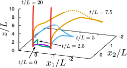
(a) $(x_{1},x_{2},z)$-space

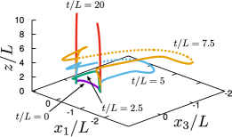
(b) $(x_{1},x_{3},z)$-space

(c) $(x_{1},x_{2},x_{3})$-space

Figure 13: Poincaré coordinate snapshots of the string dynamics for the transverse circular quench with $\epsilon=0.1$ and $\Delta t/L=2$.

In Fig. 14, the forces acting on the quark and antiquark for the transverse quenches are shown. Their behaviors are similar to the case of longitudinal quenches: The forces show power law decay in the late time as the string expands. For the transverse linear quench with $(\epsilon,\Delta t/L)=(0.15,2)$, we find that the increase of the energy by the quench is almost the same as the case of the longitudinal quench with the same parameters. The power law in $\bm{F}$ is also found $t^{-3.8}$, consistent with the corresponding longitudinal quench. The transverse circular quench shown here has a little bit smaller energy injection and a different exponent $t^{-3.7}$. The force on the antiquark also seem to behave in the same power law as the quark side. In Fig. 14(a), however, the curve of $|\bar{\bm{F}}|$ does not look to approach that of $|\bm{F}|$, but this might be because of distortion by the cusps. In contrast, Fig. 14(b) suggests that the behaviors of the forces will be similar in very late time.

In these examples of different quenches, we observe common transition to the power law tail region, and the string plunges into the Poincaré horizon once a sufficient amount of energy is supplied by the quench. Hence it looks that the the dynamical change of the string configurations is most likely governed by the strength of the perturbation and less sensitive to the details like quench patterns of dimensionality of string motions.

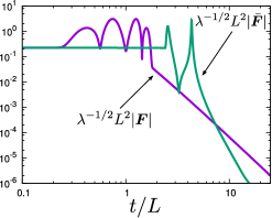
(a) Transverse linear quench

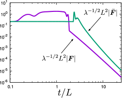
(b) Transverse circular quench

Figure 14: Forces acting on the quark and antiquark for the transverse quenches. The parameters are $(\epsilon,\Delta t/L)=(0.15,\,2)$ and $(0.1,\,2)$ for the transverse linear and circular quenches, respectively.

6 Summary and discussion

We studied strong perturbations of a fundamental string in AdS dual to the flux tube between a pair of external quark and antiquark in $\mathcal{N}=4$ super Yang-Mills theory. Non-linear perturbations were introduced to the string by shaking its endpoints. While our physical interest were in the Poincaré patch, we adopted the global patch as the target space for solving the string dynamics numerically. We found that the string plunged into the Poincaré horizon if the perturbations were strong enough. In this process, effective event horizons were dynamically created on the worldsheet before the string reached the Poincaré horizon. The condition for the string plunge was that the injected energy by a quench exceeded the potential energy of the $q$-$\bar{q}$ pair. The forces acting on the quark and antiquark were found to approach zero at late time with power law decay, whose exponent depended on the quench parameters. We argued that the presence of the power law tail might be associated with redshift effects on the string and the initial curved configuration of the string. Using the case that the string extended to the Poincaré horizon, we discussed the relationship between the power law and effects from the worldsheet effective horizons.

The slope of the power law depended on the quench parameters. As $\epsilon/\Delta t$ decreases, the exponent seems to be smaller, while it becomes difficult to observe a long-time power law tail because the string stop expanding and waves reflect between the boundaries. In the limit of $\epsilon/\Delta t\to 0$, no dynamics is induced on the string, and the exponent may also approach zero. On the other hand, for large $\epsilon/\Delta t$, the slope would be steeper. The velocity of the string endpoint by quenches reaches the speed of light at some finite $\epsilon/\Delta t$ Ishii:2015wua . In such a situation, the bulk string element adjacent to the boundary is causally disconnected, and the initial shape of the bulk string would be irrelevant to the force. In that limit, the force may drop to zero suddenly after the compact quench is over.

One of the future directions of our work is to study string dynamics in AdS black hole background. In finite temperatures, straight strings extending to the black hole represent deconfined quarks in gluon plasma Rey:1998bq ; Brandhuber:1998bs . It would be straightforward to see a nonlinarly perturbed hanging string change to straight strings extending to the black hole. In general, it is known that perturbations around AdS black holes do not show power law decay tails Horowitz:1999jd . However, while the string is heading for the black hole, power law decay would appear, at least for a sufficiently low temperature, although it may be eventually taken over by an exponential ring down due to the presence of the black hole. It would be interesting to see if a time domain of power law decay can be observed in high temperature black holes. In application of the gauge/gravity duality to strongly coupled QCD, much attention has been also given to moving quarks in Yang-Mills plasma Herzog:2006gh ; Gubser:2006bz ; CasalderreySolana:2006rq ; Gubser:2006nz ; CasalderreySolana:2007qw ; Liu:2006ug ; Liu:2006he and moving quark-antiquark pairs Liu:2006nn ; Chernicoff:2006hi . It would be interesting to apply our computational methods to study nonlinear fluctuations on quarks and mesons in strongly coupled plasmas from the viewpoint of the holographic string.

The interpretations of the disconnection of the string in the dual field theory is that the flux tube between the quark and antiquark vanish. While horizons are created on the string as if the string were broken into two, this actually is not analogous to the breaking of the flux tube in “confined” theories. In fact, $\mathcal{N}=4$ super Yang-Mills theory is conformal and not confining. What we observed in our AdS setup was that the AdS string having two static solutions transitioned from the hanging to straight strings. While this dynamical transition is calculated and observed in a simple setup of the pure AdS background in this work, this finding would have interesting implications in generalizations of this work: nonlinear perturbations of strings in confining geometries. The string may become infinitely long in confining geometries where no disconnected string configuration exists. A related study was done in Vegh:2015yua for a global AdS string whose boundary conditions are different from ours, and a phase with endlessly extending string was found when perturbations were continuously added. It would be interesting to examine if a finite perturbation can make a string stretch forever as well as create event horizons on the string.

An exact solution of an expanding string with accelerating endpoints has been found in Xiao:2008nr . This solution, having effective horizons on its worldsheet, has been regarded as the holographic dual of an Einstein-Podolsky-Rosen (EPR) pair Jensen:2013ora since the quark and antiquark pair should be color singlet (entangled) but is causally disconnected (See also Maldacena:2013xja ). In this paper, we found the dynamical horizon creation on the string worldsheet just by changing the string endpoints temporarily, and as a result the endpoints became causally disconnected. How the effective horizons shut their communication were schematically visualized in Fig. 5. It would be interesting to consider entanglement and EPR pairing in this kind of dynamical horizon formation.

Appendix A Discretization at the boundary

In this appendix, we explain the discretized evolution at the boundary in the global coordinates. This is different from the Poincaré patch’s flat boundary considered in Ishii:2015wua . While the $\chi$-coordinates are useful for solving equations in the bulk, we find it convenient to go through the polar coordinates in deriving the discretized equations at the boundary. The coordinate change between them is given by

$$\chi_{a}=\omega_{a}\tan\frac{\theta}{2}\ ,$$ (39)

where $0\leq\theta\leq\pi/2$ is the AdS radial coordinate and $\omega_{a}$ are the spherical coordinates of $S^{3}$. In terms of the polar coordinates, the constraint equations at the boundary (28) become

$$\tau_{,u}=\sqrt{\theta_{,u}{}^{2}+|\bm{\omega}_{,u}|^{2}}\ ,\quad\tau_{,v}=\sqrt{\theta_{,v}{}^{2}+|\bm{\omega}_{,v}|^{2}}\ .$$ (40)

Let us discretize (40). For simplicity, we consider one of the string’s boundaries at $u=v$; the other ($u=v+\beta_{0}$) can be handled similarly. Introducing notations $\phi_{N}=\phi(u+h,v+h),\,\phi_{E}=\phi(u,v+h),\,\phi_{W}=\phi(u+h,v)$ and $\phi_{S}=\phi(u,v)$ where $\phi$ represents the fields, we can discretize the sum of the two equations in (40) as

$$\tau_{N}-\tau_{S}=\frac{1}{2}\left(\sqrt{(\theta_{N}-\theta_{E}+\theta_{W}-\theta_{S})^{2}+|\bm{\omega}_{N}-\bm{\omega}_{E}+\bm{\omega}_{W}-\bm{\omega}_{S}|^{2}}\right.\\ \left.+\sqrt{(\theta_{N}-\theta_{W}+\theta_{E}-\theta_{S})^{2}+|\bm{\omega}_{N}-\bm{\omega}_{W}+\bm{\omega}_{E}-\bm{\omega}_{S}|^{2}}\right).$$ (41)

From the boundary condition for $\theta$, $\theta|_{u=v}=\pi/2$, we have $\theta_{N}=\theta_{S}=\pi/2$. By examining the boundary series expansions, we find $\theta_{,uv}|_{u=v}=0$ and $\bm{\omega}_{,u}|_{u=v}=\bm{\omega}_{,v}|_{u=v}$. Discretizing them, we obtain $\theta_{E}=\pi-\theta_{W}$ and $\bm{\omega}_{E}=\bm{\omega}_{W}$. Therefore, (41) becomes

$$\tau_{N} =\tau_{S}+\sqrt{(\pi-2\,\theta_{W})^{2}+|\bm{\omega}_{N}-\bm{\omega}_{S}|^{2}}$$

$$=\tau_{S}+\sqrt{(\pi-4\tan^{-1}\!|\bm{\chi}_{W}|)^{2}+|\bm{\chi}_{N}-\bm{\chi}_{S}|^{2}}\ ,$$ (42)

where we used $|\bm{\omega}_{N}-\bm{\omega}_{S}|=|\bm{\chi}_{N}-\bm{\chi}_{S}|$ on the AdS boundary and $\theta_{W}=2\tan^{-1}\!|\bm{\chi}_{W}|$ obtained from (39). By solving (42) with (26) giving $\bm{\chi}_{N}=\bm{\chi}(\tau_{N})$, we can compute the time evolution, $\tau_{N}$ and $\bm{\chi}_{N}$.

Appendix B Error analysis

In this appendix, we estimate numerical errors by checking the constraint violation. The constraint equations have been obtained in Eq. (15). To remove the coefficients diverging at the boundary, we define rescaled constraints as

$$\tilde{C}_{1}=-(1+|\bm{\chi}|^{2})^{2}\,\tau_{,u}^{2}+4|\bm{\chi}_{,u}|^{2}\ ,\quad\tilde{C}_{2}=-(1+|\bm{\chi}|^{2})^{2}\,\tau_{,v}^{2}+4|\bm{\chi}_{,v}|^{2}\ .$$ (43)

Mathematically, they should be zero in the whole computational region if we impose the constraints at the string’s boundaries and initial surface. Hence, they can be used for checking our numerical accuracy after discretization.

For visibility, we consider the constraint violation on slices on the worldsheet. We define a surface $\Sigma(v_{0})\equiv\{v=v_{0},\,0<u<\beta_{0},\,|\tau(u,v_{0})|<\pi\}$. By assembling the surfaces, we define a one-dimensional function as

$$C_{\textrm{max}}(v)=\max_{\Sigma(v)}(|\tilde{C}_{1}|,|\tilde{C}_{2}|)\ ,$$ (44)

where on each $\Sigma(v)$ we seek the maximum value of the constraint violation by varying $u$. We also take the bigger of $|\tilde{C}_{1}|$ and $|\tilde{C}_{2}|$. Let $N$ be the number of the discretization segments on $v=\textrm{const}$ surfaces. We plot $C_{\textrm{max}}(v)$ for $N=400$, $800$ and $1600$ in Fig. 15. The constraint behaves as $C_{\textrm{max}}\propto 1/N^{2}$, consistent with our second-order discretization scheme. In the paper, we basically choose $N=1600$ for which the constraint violation is less than $10^{-3}$.

(a) Longitudinal

(b) Transverse linear

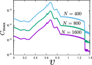
(c) Transverse circular

Figure 15: Constraint violation for several resolutions, $N=400$, $800$ and $1600$. (a) Longitudinal quench with $\epsilon=0.15$ and $\Delta t/L=2$. (b) Transverse linear quench with $\epsilon=0.15$ and $\Delta t/L=2$. (c) Transverse circular quench with $\epsilon=0.1$ and $\Delta t/L=2$.

References

- (1) J. M. Maldacena, The Large N limit of superconformal field theories and supergravity, Int.J.Theor.Phys. 38 (1999) 1113–1133, [hep-th/9711200].
- (2) S. Gubser, I. R. Klebanov, and A. M. Polyakov, Gauge theory correlators from noncritical string theory, Phys.Lett. B428 (1998) 105–114, [hep-th/9802109].
- (3) E. Witten, Anti-de Sitter space and holography, Adv.Theor.Math.Phys. 2 (1998) 253–291, [hep-th/9802150].
- (4) P. M. Chesler and L. G. Yaffe, Horizon formation and far-from-equilibrium isotropization in supersymmetric Yang-Mills plasma, Phys.Rev.Lett. 102 (2009) 211601, [arXiv:0812.2053].
- (5) P. M. Chesler and L. G. Yaffe, Boost invariant flow, black hole formation, and far-from-equilibrium dynamics in N = 4 supersymmetric Yang-Mills theory, Phys.Rev. D82 (2010) 026006, [arXiv:0906.4426].
- (6) P. M. Chesler and L. G. Yaffe, Holography and colliding gravitational shock waves in asymptotically AdS5 spacetime, Phys.Rev.Lett. 106 (2011) 021601, [arXiv:1011.3562].
- (7) P. M. Chesler and L. G. Yaffe, Numerical solution of gravitational dynamics in asymptotically anti-de Sitter spacetimes, JHEP 07 (2014) 086, [arXiv:1309.1439].
- (8) P. M. Chesler and L. G. Yaffe, Holography and off-center collisions of localized shock waves, JHEP 10 (2015) 070, [arXiv:1501.04644].
- (9) T. Ishii, S. Kinoshita, K. Murata, and N. Tanahashi, Dynamical Meson Melting in Holography, JHEP 04 (2014) 099, [arXiv:1401.5106].
- (10) K. Hashimoto, S. Kinoshita, K. Murata, and T. Oka, Electric Field Quench in AdS/CFT, JHEP 09 (2014) 126, [arXiv:1407.0798].
- (11) K. Hashimoto, S. Kinoshita, K. Murata, and T. Oka, Turbulent meson condensation in quark deconfinement, Phys. Lett. B746 (2015) 311–314, [arXiv:1408.6293].
- (12) K. Hashimoto, S. Kinoshita, K. Murata, and T. Oka, Meson turbulence at quark deconfinement from AdS/CFT, Nucl. Phys. B896 (2015) 738–762, [arXiv:1412.4964].
- (13) M. Ali-Akbari, F. Charmchi, A. Davody, H. Ebrahim, and L. Shahkarami, Time-dependent meson melting in an external magnetic field, Phys. Rev. D91 (2015) 106008, [arXiv:1503.04439].
- (14) T. Ishii and K. Murata, Turbulent strings in AdS/CFT, JHEP 06 (2015) 086, [arXiv:1504.02190].
- (15) S.-J. Rey and J.-T. Yee, Macroscopic strings as heavy quarks in large N gauge theory and anti-de Sitter supergravity, Eur.Phys.J. C22 (2001) 379–394, [hep-th/9803001].
- (16) J. M. Maldacena, Wilson loops in large N field theories, Phys.Rev.Lett. 80 (1998) 4859–4862, [hep-th/9803002].
- (17) J. Callan, Curtis G. and A. Guijosa, Undulating strings and gauge theory waves, Nucl.Phys. B565 (2000) 157–175, [hep-th/9906153].
- (18) I. R. Klebanov, J. M. Maldacena, and C. B. Thorn, III, Dynamics of flux tubes in large N gauge theories, JHEP 04 (2006) 024, [hep-th/0602255].
- (19) S. D. Avramis, K. Sfetsos, and K. Siampos, Stability of strings dual to flux tubes between static quarks in N = 4 SYM, Nucl.Phys. B769 (2007) 44–78, [hep-th/0612139].
- (20) R. E. Arias and G. A. Silva, Wilson loops stability in the gauge/string correspondence, JHEP 01 (2010) 023, [arXiv:0911.0662].
- (21) K. Hashimoto, M. Nishida, and A. Sonoda, Universal Turbulence on Branes in Holography, JHEP 08 (2015) 135, [arXiv:1504.07836].
- (22) N. Callebaut, S. S. Gubser, A. Samberg, and C. Toldo, Segmented strings in AdS3, JHEP 11 (2015) 110, [arXiv:1508.07311].
- (23) D. Vegh, The broken string in anti-de Sitter space, arXiv:1508.06637.
- (24) D. Vegh, Colliding waves on a string in AdS3, arXiv:1509.05033.
- (25) G. T. Horowitz and V. E. Hubeny, Quasinormal modes of AdS black holes and the approach to thermal equilibrium, Phys. Rev. D62 (2000) 024027, [hep-th/9909056].
- (26) S. Aretakis, Stability and Instability of Extreme Reissner-Nordstróm Black Hole Spacetimes for Linear Scalar Perturbations I, Commun. Math. Phys. 307 (2011) 17–63, [arXiv:1110.2007].
- (27) S. Aretakis, Stability and Instability of Extreme Reissner-Nordstrom Black Hole Spacetimes for Linear Scalar Perturbations II, Annales Henri Poincare 12 (2011) 1491–1538, [arXiv:1110.2009].
- (28) J. Lucietti, K. Murata, H. S. Reall, and N. Tanahashi, On the horizon instability of an extreme Reissner-Nordstróm black hole, JHEP 03 (2013) 035, [arXiv:1212.2557].
- (29) K. Murata, H. S. Reall, and N. Tanahashi, What happens at the horizon(s) of an extreme black hole?, Class. Quant. Grav. 30 (2013) 235007, [arXiv:1307.6800].
- (30) A. Mikhailov, Nonlinear waves in AdS / CFT correspondence, hep-th/0305196.
- (31) M. Ali-Akbari, F. Charmchi, A. Davody, H. Ebrahim, and L. Shahkarami, Evolution of Potential in N=4 Super Yang-Mills Plasma, arXiv:1510.00212.
- (32) S.-J. Rey, S. Theisen, and J.-T. Yee, Wilson-Polyakov loop at finite temperature in large N gauge theory and anti-de Sitter supergravity, Nucl.Phys. B527 (1998) 171–186, [hep-th/9803135].
- (33) A. Brandhuber, N. Itzhaki, J. Sonnenschein, and S. Yankielowicz, Wilson loops in the large N limit at finite temperature, Phys.Lett. B434 (1998) 36–40, [hep-th/9803137].
- (34) C. P. Herzog, A. Karch, P. Kovtun, C. Kozcaz, and L. G. Yaffe, Energy loss of a heavy quark moving through N=4 supersymmetric Yang-Mills plasma, JHEP 07 (2006) 013, [hep-th/0605158].
- (35) S. S. Gubser, Drag force in AdS/CFT, Phys.Rev. D74 (2006) 126005, [hep-th/0605182].
- (36) J. Casalderrey-Solana and D. Teaney, Heavy quark diffusion in strongly coupled N=4 Yang-Mills, Phys.Rev. D74 (2006) 085012, [hep-ph/0605199].
- (37) S. S. Gubser, Momentum fluctuations of heavy quarks in the gauge-string duality, Nucl.Phys. B790 (2008) 175–199, [hep-th/0612143].
- (38) J. Casalderrey-Solana and D. Teaney, Transverse Momentum Broadening of a Fast Quark in a N=4 Yang Mills Plasma, JHEP 04 (2007) 039, [hep-th/0701123].
- (39) H. Liu, K. Rajagopal, and U. A. Wiedemann, Calculating the jet quenching parameter from AdS/CFT, Phys.Rev.Lett. 97 (2006) 182301, [hep-ph/0605178].
- (40) H. Liu, K. Rajagopal, and U. A. Wiedemann, Wilson loops in heavy ion collisions and their calculation in AdS/CFT, JHEP 03 (2007) 066, [hep-ph/0612168].
- (41) H. Liu, K. Rajagopal, and U. A. Wiedemann, An AdS/CFT Calculation of Screening in a Hot Wind, Phys.Rev.Lett. 98 (2007) 182301, [hep-ph/0607062].
- (42) M. Chernicoff, J. A. Garcia, and A. Guijosa, The Energy of a Moving Quark-Antiquark Pair in an N=4 SYM Plasma, JHEP 09 (2006) 068, [hep-th/0607089].
- (43) B.-W. Xiao, On the exact solution of the accelerating string in AdS(5) space, Phys. Lett. B665 (2008) 173–177, [arXiv:0804.1343].
- (44) K. Jensen and A. Karch, Holographic Dual of an Einstein-Podolsky-Rosen Pair has a Wormhole, Phys.Rev.Lett. 111 (2013), no. 21 211602, [arXiv:1307.1132].
- (45) J. Maldacena and L. Susskind, Cool horizons for entangled black holes, Fortsch. Phys. 61 (2013) 781–811, [arXiv:1306.0533].