Density functional theory of gas-liquid phase separation in dilute binary mixtures

Abstract

We examine statics and dynamics of phase-separated states of dilute binary mixtures using density functional theory. In our systems, the difference in the solvation chemical potential $\Delta\mu_{s}$ between liquid and gas is considerably larger than the thermal energy $k_{B}T$ for each solute particle and the attractive interaction among the solute particles is weaker than that among the solvent particles. In these conditions, the saturated vapor pressure increases by an amount equal to the solute density in liquid multiplied by the large factor $k_{B}T\exp(\Delta\mu_{s}/k_{B}T)$. As a result, phase separation is induced at low solute densities in liquid and the new phase remains in gaseous states, while the liquid pressure is outside the coexistence curve of the solvent. This explains the widely observed formation of stable nanobubbles in ambient water with a dissolved gas. We calculate the density and stress profiles across planar and spherical interfaces, where the surface tension decreases with increasing the interfacial solute adsorption. We realize stable solute-rich bubbles with radius about 30 nm, which minimize the free energy functional. We then study dynamics around such a bubble after a decompression of the surrounding liquid, where the bubble undergoes a damped oscillation. In addition, we present some exact and approximate expressions for the surface tension and the interfacial stress tensor.

I Introduction

Much attention has been paid to complex interactions among dissolved particles and solvent molecules Likos ; Hansen ; Hop . In liquid water, hydrophobic particles deform the surrounding hydrogen bond structureChandler ; Garde ; Paul , resulting in a solvation chemical potential $\mu_{s}$ much larger than the thermal energy $k_{B}T$ (per particle). As a result, they tend to aggregate in liquid water at ambient conditions (room temperature and 1 atm pressure). In simulations of a hard-sphere particle with radius $a$ in ambient water, $\mu_{s}$ is of order $4\pi a^{2}\sigma$ for $a>1$ nm, where $\sigma$ is the gas-liquid surface tension Chandler ; Garde ; Paul . Such large particles are thus strongly hydrophobic ($\mu_{s}\sim 180k_{B}T$ for $a\sim 1$ nm). Another notable example is the solvent-mediated interaction among colloidal particles in near-critical mixture solvents Es ; Beysens ; Dietrich ; Oka1 ; Tanaka ; Araki ; Yabu ; Furu , where one fluid component is preferentially adsorbed on the colloidal surfaces, largely deforming the surrounding critical fluctuations and often leading to local phase separation (bridging).

Recently, we have presented a theory on the formation of small bubbles in ambient water containing a small amount of a dissolved gas nano . As a typical example, O₂ is mildly hydrophobic with $\mu_{s}=3.44k_{B}T$ in liquid water at $T=300$ K. As a unique feature of ambient liquid water, it has pressures only slightly higher than the saturated vapor pressure or is immediately outside the coexistence curve (CX) in the phase diagram. Moreover, the van der Waals interaction among O₂ molecules is relatively weak as compared to the hydrogen bond interaction. In fact, the critical temperature of water is considerably higher than that of O₂ (647.3 K for water and 154.6 K for O₂). In this situation, O₂ molecules tend to be expelled from liquid water in the form of oxygen-rich bubbles (or films) above a very low threshold concentration outside CX. In many experiments, small bubbles, often called nanobubbles, have been observed in the bulk and on hydrophobic walls in ambient water review1 ; review2 . Their radius is typically of order $10-100$ nm and their life time is very long. In our theorynano , they are thermodynamically stable, minimizing the free energy including the surface tension. As a similar phenomenon, long-lived heterogeneities have been observed in one-phase states of aqueous mixtures with addition of a small amount of a salt or a hydrophobic soluteAni ; Oka-p ; Bu . These phenomena emerge as examples of selective solvation effectsBu .

In this paper, we investigate two-phase states of dilute binary mixtures at $T=300$ K using the density functional theory (DFT) Hop ; Tara ; Sullivan ; Evansreview ; Lutsko on the basis of the Carnahan-Starling model for binary mixtures Car0 ; Car . As in the case of O₂ in water, we determine the model parameters in Ref.Car such that $\mu_{s}$ is $3.44k_{B}T$ in liquid and the solute-solute attractive interaction is weaker than that among the solvent particles. In these conditions, we consider gas-liquid coexistence separated by planar and spherical interfaces, where we calculate the density and stress profiles and the solute-induced deviations of thermodynamic quantities. For our parameter values, there also arises a significant interfacial adsorption of the solute, which leads to a reduction of the surface tension $\sigma$ in accord with the Gibbs law Gibbs . We are interested in stable solute-induced bubbles minimizing the free energy functional of DFT. The radius of a stable bubble $R_{m}$ is larger than the critical radius of nucleation $R_{c}$Katz ; Caupin ; Langer ; Onukibook , but remains to be vey small.

Within the scheme of DFT, some attempts have been made to describe dynamics of colloidal particles in solvent without Marconi ; Archer-Evans and with Lowen ; Lutsko ; Goddard ; Donev the hydrodynamic interaction. We also mention dynamic van der Waals theory with gradient entropy and energy vanderOnuki , which is a generalization of the original van der Waals theoryvander . Using this scheme, Teshigawara and one of the present authors (A.O.) numerically studied evaporation and condensation in inhomogeneous temperatureTeshi ; Teshi1 ; Teshi2 . In their simulations, Tanaka and Araki treated colloidal particles as highly viscous droplets with diffuse interfaces Tanaka . Their method has been used to study hydrodynamics and phase separation around colloidal particles Tanaka ; Araki ; Furu ; Yabu . In this paper, we present dynamic equations for binary mixtures composed of small particles, where DFT and hydrodynamics are incorporated on acoustic and diffusive timescales. As an application, we study dynamics around a bubble after a decompression of the surrounding liquid.

Bubble dynamics is very complicated, where hydrodynamics and gas-liquid phase transition are inseparably coupled Plesset ; Nepp ; Szeri ; sonol . On short timescales, the pressure balance does not hold at the interface and the bubble motions become oscillatory accompanied by acoustic disturbances. In particular, they have been studied extensively under applied acoustic field. On long timescales, the bubble growth is governed by the thermal diffusion in one-component fluids Langer ; Onukibook and by the slower solute diffusion in mixtures Szeri ; nano . In this paper, we aim to study these characteristic features.

This paper is organized as follows. In Sec.II, we will present the background of DFT related to our problem. In Sec.III, we will examine two-phase states of dilute binary mixtures including a considerably large solvation chemical potential in DFT. In Sec.IV, dynamics around a bubble will be studied numerically. In Appendix B, we will present some relations for the interfacial stress tensor in the exact statistical theory.

II Theoretical background

II.1 Free energy functional

We treat a neutral binary mixture in DFT Sullivan ; Evansreview ; Tara ; Lutsko , where the first species is a solvent and the second one is a dilute solute. The number densities $n_{1}({\mbox{\boldmath$r$}})$ and $n_{2}({\mbox{\boldmath$r$}})$ are coarse-grained smooth functions of space. There are no Coulombic and dipolar interactions. Hereafter, the temperature $T$ is assumed to be a homogeneous constant ($=300$ K) and the Boltzmann constant is set equal to 1.

In DFT, the Helmholtz free energy functional consists of two parts as ${\cal F}={\cal F}_{h}+{\cal F}_{a}$. The first part is of the local form ${\cal F}_{h}=\int d{\mbox{\boldmath$r$}}f(n_{1},n_{2})$ with the free energy density,

$$f=T\sum_{i}n_{i}[\ln(n_{i}\lambda_{i}^{3})-1]+f_{h}(n_{1},n_{2})+\sum_{i}n_{i}U_{i},$$ (1)

where $\lambda_{i}(\propto T^{-1/2})$ is the thermal de Broglie length and the space integral is within the cell. The $f_{h}(n_{1},n_{2})$ arises from the short-ranged repulsive interaction and is taken to assume the binary Carnahan-Starling formCar . See Appendix A for its details. The $U_{i}({\mbox{\boldmath$r$}})$ is the externally applied potential such as the wall or gravitational potential. The second part ${\cal F}_{a}$ arises from the attractive interaction and is of the form,

$${\cal F}_{a}=\frac{1}{2}\int d{\mbox{\boldmath$r$}}_{1}\int d{\mbox{\boldmath$r$}}_{2}\sum_{i,j}\phi_{ij}(r_{12})n_{i}({\mbox{\boldmath$r$}}_{1})n_{j}({\mbox{\boldmath$r$}}_{2}).$$ (2)

Here, $\phi_{ij}(r_{12})$ is an effective potential, which is negative and continuously depends on the distance $r_{12}=|{\mbox{\boldmath$r$}}_{1}-{\mbox{\boldmath$r$}}_{2}|$. Its space integral should be finite, so we introduce

$$w_{ij}=-4\pi\int_{0}^{\infty}drr^{2}\phi_{ij}(r).$$ (3)

We define the chemical potentials of the two species as the functional derivatives $\mu_{i}({\mbox{\boldmath$r$}})=\delta{\cal F}/\delta n_{i}({\mbox{\boldmath$r$}})$. For the present model they are expressed as

$$\mu_{i}=T\ln(n_{i}\lambda_{i}^{3})+\mu_{hi}+\mu_{ai}+U_{i},$$ (4)

where $\mu_{hi}={\partial f_{h}}/{\partial n_{i}}$ is the repulsive part and $\mu_{ai}$ is the attractive part expressed in the convolution form as

$$\mu_{ai}=\int d{\mbox{\boldmath$r$}}_{1}\sum_{j}\phi_{ij}(r_{1})n_{j}({\mbox{\boldmath$r$}}-{\mbox{\boldmath$r$}}_{1}).$$ (5)

For homogeneous $n_{j}$ we have $\mu_{ai}=-\sum_{j}w_{ij}n_{j}$.

If variations of $n_{i}$ are sufficiently slow, we can use the gradient expansion of ${\cal F}_{a}$ Evansreview ; Cahn ; Onukibook to obtain ${\cal F}_{a}\cong\int d{\mbox{\boldmath$r$}}\sum_{ij}[-w_{ij}n_{i}n_{j}/2+C_{ij}\nabla n_{i}\cdot{\nabla n_{j}}/2]$, where

$$C_{ij}=-\frac{2\pi}{3}\int_{0}^{\infty}drr^{4}\phi_{ij}(r).$$ (6)

With this approximation, we recognize the relationship between DFT and the original van der Waals theory with the gradient free energyvander .

In the literatureEvansreview ; Tara ; Lutsko , $\phi_{ij}(r)$ has often been set equal to the attractive part of the Lennard-Jones potential characterized by the parameters $d_{ij}$ and $\epsilon_{ij}$. For $r>2^{1/6}d_{ij}$ it is expressed as

$$\phi_{ij}(r)=4\epsilon_{ij}[(d_{ij}/r)^{12}-(d_{ij}/r)^{6}],$$ (7)

For $r\leq 2^{1/6}d_{ij}$, we define $\phi_{ij}(r)=-\epsilon_{ij}$. In our numerical analysis, at $T=300$ K, we set

$$d_{1}=d_{11}=3.0~{}{\rm\AA},~{}d_{2}=d_{22}=2.48~{}{\rm\AA},~{}d_{12}=2.74~{}{\rm\AA},$$

$$\epsilon_{11}=588.76~{}{\rm K},~{}\epsilon_{22}=108.53~{}{\rm K},~{}\epsilon_{12}=251.26~{}{\rm K}.$$ (8)

Hereafter, we write $d_{1}=d_{11}$ and $d_{2}=d_{22}$ for simplicity. From Eq.(3) these values lead to $w_{11}/d_{1}^{3}T=30.80$, $w_{22}/d_{1}^{3}T=3.21$, and $w_{12}/d_{1}^{3}T=10.02$. Here, $\epsilon_{22}/\epsilon_{11}=0.18$, so the solute-solute attractive interaction is much weaker than the solvent-solvent one. This is one of the conditions of the solute-induced bubble formationnano . In two-phase coexistence of the first species, the liquid and gas densities are calculated as $n_{\ell}=1.0d_{1}^{-3}=37$ nm^-3 and $n_{g}=2.05\times 10^{-5}d_{1}^{-3}=7.7\times 10^{-4}$ nm^-3. On the other hand, in real ambient water, they are known to be $n_{\ell}\sim 33$ nm^-3 and $n_{g}\sim 10^{-3}$ nm^-3.

II.2 Stress tensor in DFT

We examine the stress tensor $\Pi_{\alpha\beta}({\mbox{\boldmath$r$}})$ ($\alpha,\beta=x,y,z$) in DFT. If $f_{h}$ is of the local form, the repulsive part of $\Pi_{\alpha\beta}$ is diagonal as $p_{h}\delta_{\alpha\beta}$ with

$$p_{h}=n_{1}\mu_{h1}+n_{2}\mu_{h2}-f_{h}.$$ (9)

However, the attractive pair interaction gives rise to off-diagonal components. We express $\Pi_{\alpha\beta}$ as

$$\Pi_{\alpha\beta}=(Tn+p_{h})\delta_{\alpha\beta}-\int d{\mbox{\boldmath$r$}}_{1}\int d{\mbox{\boldmath$r$}}_{2}\sum_{ij}\frac{x_{12\alpha}x_{12\beta}}{2r_{12}}$$

$$\times\phi^{\prime}_{ij}(r_{12})\delta_{s}({\mbox{\boldmath$r$}},{\mbox{\boldmath$r$}}_{1},{\mbox{\boldmath$r$}}_{2})n_{i}({\mbox{\boldmath$r$}}_{1})n_{j}({\mbox{\boldmath$r$}}_{2}),$$ (10)

where $n=n_{1}+n_{2}$, $\phi^{\prime}_{ij}=d\phi_{ij}/dr$, and $x_{12\alpha}=x_{1\alpha}-x_{2\alpha}$. We use the Irving-Kirkwood $\delta$ functionIrving ; Kirk ; Scho ; Onukibook ,

$$\delta_{s}({\mbox{\boldmath$r$}},{\mbox{\boldmath$r$}}_{1},{\mbox{\boldmath$r$}}_{2})=\int_{0}^{1}d\lambda\delta({\mbox{\boldmath$r$}}-\lambda,{\mbox{\boldmath$r$}}_{1}-(1-\lambda){\mbox{\boldmath$r$}}_{2}),$$ (11)

which is nonvanishing only when $r$ is on the line segment connecting ${\mbox{\boldmath$r$}}_{1}$ and ${\mbox{\boldmath$r$}}_{2}$. The integrand is appreciable only if $|{\mbox{\boldmath$r$}}-{\mbox{\boldmath$r$}}_{1}|$ and $|{\mbox{\boldmath$r$}}-{\mbox{\boldmath$r$}}_{2}|$ are shorter than the potential range. The expression (10) is approximate, while the exact one in terms of $\delta_{s}$ Irving will be given in Appendix B.

Using ${\mbox{\boldmath$r$}}_{12}\cdot\nabla\delta_{s}({\mbox{\boldmath$r$}},{\mbox{\boldmath$r$}}_{1},{\mbox{\boldmath$r$}}_{2})=\delta({\mbox{\boldmath$r$}}-{\mbox{\boldmath$r$}}_{2})-\delta({\mbox{\boldmath$r$}}-{\mbox{\boldmath$r$}}_{1})$ and $\phi_{ij}^{\prime}(r_{12})x_{12\alpha}/r_{12}=\partial\phi_{ij}(r_{12})/\partial x_{1\alpha}$, we find

$$\sum_{\beta}\nabla_{\beta}\Pi_{\alpha\beta}=\sum_{i}n_{i}\nabla_{\alpha}(\mu_{i}-U_{i}),$$ (12)

where $\nabla_{\beta}=\partial/\partial x_{\beta}$. This relation holds generally for homogeneous $T$ (even in nonequilibrium). In equilibrium, $\mu_{1}$ and $\mu_{2}$ are homogeneous, which leads to the mechanical equilibrium condition $\sum_{\beta}\nabla_{\beta}\Pi_{\alpha\beta}+\sum_{i}n_{i}\nabla_{\alpha}U_{i}=0$ from Eq.(12). For homogeneous $n_{i}$, we have the diagonal form $\Pi_{\alpha\beta}=(Tn+p_{h}-\sum_{ij}w_{ij}n_{i}n_{j}/2)\delta_{\alpha\beta}$ as in the van der Waals theoryOnukibook ; vander .

II.3 Equilibrium in one-dimensional geometry

We assume that our fluid is between parallel walls separated by $L$. The wall area much exceeds $L^{2}$. The $U_{i}$ in Eq.(1) is the wall potential. Then, all the physical quantities depend only on $z$. We do not consider capillary wave fluctuations, which are inhomogeneous in the $xy$ plane on large scales. They are known to give rise to broadening of the profile Sti ; Evansreview ; Grest .

II.3.1 Pressure balance and grand potential

In equilibrium, the chemical potentials in Eq.(4) are homogeneous in the cell as $\mu_{1}=\mu_{1}^{0}$ and $\mu_{2}=\mu_{2}^{0}$, where $\mu_{1}^{0}$ and $\mu_{2}^{0}$ are constants. After integration in the $xy$ plane, the attractive part $\mu_{ai}$ in Eq.(5) becomes

$$\mu_{ai}(z)=2\pi\sum_{j}\int dz_{1}\Phi_{ij}(z-z_{1})n_{j}(z_{1}),$$ (13)

where we define the function,

$$\Phi_{ij}(z)=\int_{|z|}^{\infty}drr\phi_{ij}(r).$$ (14)

Here, $\int dz\Phi_{ij}(z)=2\int_{0}^{\infty}drr^{2}\phi_{ij}(r)=-w_{ij}/2\pi$, so we have $\mu_{ai}=-\sum_{j}w_{ij}n_{j}$ for homogeneous $n_{j}$.

From Eq.(12) the stress balance along the $z$ axis gives

$$\frac{d}{dz}\Pi_{zz}=-\sum_{i}n_{i}U_{i}^{\prime},$$ (15)

where $U_{i}^{\prime}=dU_{i}/dz$ and $\Pi_{zz}$ consists of three parts as

$$\Pi_{zz}(z)=Tn(z)+p_{h}(z)+p_{a}(z).$$ (16)

From Eq.(10) the attractive part $p_{a}$ is expressed as

$$p_{a}=2\pi\int_{z}^{L}dz_{1}\int_{0}^{z}dz_{2}\sum_{ij}z_{12}\phi_{ij}(z_{12})n_{i}(z_{1})n_{j}(z_{2}),$$ (17)

where $z_{12}=z_{1}-z_{2}$ and $z_{2}<z<z_{1}$ in the integrand. Here, use has been made of the relation,

$$\int d{\mbox{\boldmath$r$}}_{1\perp}\delta_{s}({\mbox{\boldmath$r$}},{\mbox{\boldmath$r$}}_{1},{\mbox{\boldmath$r$}}_{2})=[\theta(z-z_{2})-\theta(z-z_{1})]/z_{12},$$ (18)

where $d{\mbox{\boldmath$r$}}_{1\perp}=dx_{1}dy_{1}$ and $\theta(u)$ is the step function ( equal to 1 for $u>0$ and to 0 for $u\leq 0$). From Eq.(15), $\Pi_{zz}$ is homogeneous far from the walls and its value is written as $p^{0}_{\rm b}$. This means that if two phases are separated by a planar interface far from the walls, the pressures in the bulk two regions are commonly given by $p^{0}_{\rm b}$.

The grand potential $\Omega=\int d{\mbox{\boldmath$r$}}\omega$ is the space integral of its density $\omega$. In the present 1D case, we find

$$\omega = f+\frac{1}{2}\sum_{i}\mu_{ai}n_{i}-\sum_{i}\mu_{i}n_{i}$$ (19)

$$= -\Pi_{zz}+p_{a}-\frac{1}{2}\sum_{i}\mu_{ai}n_{i}.$$

In the second line, use has been made of Eqs.(13), (16), and (17). In the bulk, both $p_{a}$ and $\sum_{ij}n_{i}\mu_{ai}/2$ tend to $-\sum_{ij}w_{ij}n_{i}n_{j}/2$. Hence, $\omega$ deviates from its bulk value $-p^{0}_{\rm b}$ only near the interface or the walls.

Figure 1: Left: Densities $n_{1}(z)$ and $n_{2}(z)$ vs $z/d_{1}$ around planar interfaces at $T=300$ K far below the criticality. Solvent and solute densities $(n_{1}^{\ell},n_{2}^{\ell},n_{1}^{g},n_{2}^{g})$ in bulk liquid and gas are (a) $(1.0,0,2.05\times 10^{-5},0)$ (without solute), (b) $(1.0,6.24\times 10^{-4},2.40\times 10^{-5},2.02\times 10^{-2})$ , and (c) $(1.0,2.71\times 10^{-3},4.28\times 10^{-5},0.097)$ in units of $d_{1}^{-3}$. In (b) and (c) (inset), numerical $n_{2}(z)$ (bold line) is compared with low density expression in Eq.(37) (dotted line) around the adsorption peak. Right: Stress difference $\Delta\Pi(z)=\Pi_{zz}(z)-\Pi_{xx}(z)$ divided by $p_{0}=Td_{1}^{-3}=153$ MPa vs $z/d_{1}$, calculated from Eqs.(27) and (28) for (a), (b), and (c). Its integral is the surface tension $\sigma$, which is (a) $4.00(=\sigma_{0})$, (b) $3.85$, and (c) $3.40$ in units of $Td_{1}^{-2}$. The coexisting pressure $p_{\rm cx}$ is (a) $2.1\times 10^{-5}(=p_{\rm cx}^{0})$, (b) $2.0\times 10^{-2}$, and (c) $0.094$ in units of $Td_{1}^{-3}$. Vertical broken lines indicate the position of the Gibbs dividing surface in Eq.(20).

II.3.2 Surface tension

Let a planar interface parallel to the $xy$ plane separate gas and liquid phases far from the walls, where $U_{i}=0$ and $\Pi_{zz}=p_{\rm cx}=$const. around the interface, where $p_{\rm cx}$ is the coexisting (saturated pressure) of the mixture. The left panels of Fig.1 display equilibrium density profiles $n_{1}(z)$ and $n_{2}(z)$, which are calculated from the method in Appendix C. They tend to $n_{1}^{\ell}$ and $n_{2}^{\ell}$ in liquid ($z-z_{\rm int}\gg d_{1})$and $n_{1}^{g}$ and $n_{2}^{g}$ in gas ($z_{\rm int}-z\gg d_{1})$, respectively. We can determine the interface position $z_{\rm int}$ by

$$z_{\rm int}=\int_{0}^{L}dz[n_{1}(z)-n_{1}^{g}]/[n_{1}^{\ell}-n_{1}^{g}],$$ (20)

using the solvent density profile $n_{1}(z)$Gibbs . Note that $n_{1}^{\ell}$ is nearly fixed at $1.0d_{1}^{-3}$ because the liquid compressibility is small.

From Eq.(19), the surface tension $\sigma$ is the $z$-integral of of $p_{a}-\sum_{i}n_{i}\mu_{ai}/2$. Thus, Eqs.(13) and (17) gives

$$\sigma=\frac{1}{2}\int dz_{1}\int dz_{2}\sum_{ij}\Theta_{ij}(z_{12})n_{i}(z_{1})n_{j}(z_{2}),$$ (21)

where we define the function,

$$\Theta_{ij}(z)=2\pi[z^{2}\phi_{ij}(|z|)-\Phi_{ij}(z)].$$ (22)

Here, from $\int dz\Theta_{ij}(z)=0$, we can replace $n_{i}(z_{1})n_{j}(z_{2})$ by $[n_{i}(z_{1})-n_{i}(z_{2})][n_{j}(z_{2})-n_{j}(z_{1})]/2$ in Eq.(21); then, the integrand is nonvanishing only near the interface. See Appendix B for the exact formula for $\sigma$ Kirk .

Furthermore, we introduce another function $K_{ij}(z)$ by

$$K_{ij}(z)=\frac{\pi}{2}\int^{\infty}_{|z|}drr(z^{2}-r^{2})\phi_{ij}(r).$$ (23)

This function is related to $\Phi_{ij}$ and $\Theta_{ij}$ as

$$\frac{d}{dz}K_{ij}(z)=\pi z\Phi_{ij}(z),\quad\frac{d^{2}}{dz^{2}}K_{ij}(z)=-\frac{1}{2}\Theta_{ij}(z).$$ (24)

In terms of $K_{ij}$ and $n_{i}^{\prime}=dn_{i}/dz$, $\sigma$ is expressed as

$$\sigma=\int dz_{1}\int dz_{2}\sum_{ij}K_{ij}(z_{12})n_{i}^{\prime}(z_{1})n_{j}^{\prime}(z_{2}).$$ (25)

This leads to the well-known form $\sigma=\int dz\sum_{ij}C_{ij}n^{\prime}_{i}n_{j}^{\prime}$ in the gradient theory Onukibook ; Cahn ; Evansreview , where $\int dzK_{ij}(z)=C_{ij}$ from Eqs.(6) and (23). If we assume the Lennard-Jones form in Eq.(7), we have $K_{ij}(z)\sim|z|^{-2}$, $\Phi_{ij}(z)\sim|z|^{-4}$, and $\Theta_{ij}(z)\sim|z|^{-4}$ for large $|z|\gg d_{1}$.

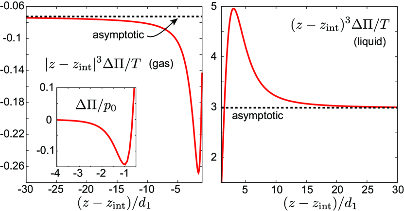
Figure 2: $|z-z_{\rm int}|^{3}\Delta\Pi(z)/T$ vs $(z-z_{\rm int})/d_{1}$ in gas (left) and liquid (right) for case (c) in Fig.1 with $n_{2}^{\ell}=4.28\times 10^{-5}d_{1}^{-3}$. It tends to $-0.0721$(left) and to $3.00$ (left) in agreement with Eq.(29). In the inset (left) $\Delta\Pi/p_{0}$ is expanded in gas, which has a small negative minimum.

The surface tension $\sigma$ of neutral fluids can generally be expressed by the Bakker formulaBakker ; Ono ; Kirk ; Evansreview ,

$$\sigma=\int dz[\Pi_{zz}(z)-\Pi_{xx}(z)]=\int dz\Delta\Pi(z).$$ (26)

The stress difference $\Delta\Pi(z)\equiv\Pi_{zz}(z)-\Pi_{xx}(z)$ is nonvanishing only near the interface. In DFT, we start with Eq.(10) and use Eq.(18) to obtain

$$\Delta\Pi(z)=\int_{z}^{L}dz_{1}\int_{0}^{z}dz_{2}\sum_{ij}\frac{\Theta_{ij}(z_{12})}{z_{12}}n_{i}(z_{1})n_{j}(z_{2}),$$ (27)

where $z_{1}>z>z_{2}$ in the integrand. With respect to $z$, integration of $\Delta\Pi(z)$ in Eq.(27) gives Eq.(21), while its derivative is written in the single integral form,

$$\frac{d\Delta\Pi}{dz}=\int_{0}^{\infty}d\xi\sum_{ij}\frac{\Theta_{ij}(\xi)}{\xi}[n_{i}(z+\xi)-n_{i}(z-\xi)]n_{j}(z).$$ (28)

Far from the interface, $\Delta\Pi(z)$ decays as $\propto|z-z_{\rm int}|^{-3}$ if the Lennard-Jones potential in Eq.(7) is assumed. In Eq.(28), we may replace $[n_{i}(z+\xi)-n_{i}(z-\xi)]n_{j}(z)$ by $(n_{i}^{\ell}-n_{i}^{g})n_{j}^{\ell}$ for $\xi>z-z_{\rm int}\gg d_{1}$. Then, for $z-z_{\rm int}\gg d_{1}$, we find $d\Delta\Pi(z)/dz\sim|z-z_{\rm int}|^{-4}$ and

$$\Delta\Pi(z)\cong\frac{\pi}{2}\sum_{ij}\epsilon_{ij}d_{ij}^{6}(n_{i}^{\ell}-n_{i}^{g})n_{j}^{\ell}|z-z_{\rm int}|^{-3}.$$ (29)

In the gas side with $z_{\rm int}-z\gg d_{1}$, the corresponding tail is obtained if $n_{j}^{\ell}$ in Eq.(29) is replaced by $-n_{j}^{g}$. Thus, its amplitude becomes very small in the gas side. Remarkably, the above form of $\Delta\Pi(z)$ holds exactly for Lennard-Jones systems (see Appendix B). Note that the density profiles $n_{i}(z)$ themselves decay as $|z-z_{\rm int}|^{-3}$, as will be shown in Eqs.(43)-(45) Tara ; Baker ; Hauge . In contrast, in the gradient theory, we have $\Delta\Pi(z)=\sum_{ij}C_{ij}n_{i}^{\prime}(z)n_{j}^{\prime}(z)$ Onukibook , which decays exponentially far from the interface.

In the right panels of Fig.1, we plot $\Delta\Pi(z)$ calculated from Eq.(28), where its integral ($=\sigma$) decreases with increasing the solute amount due to its interfacial adsorption (see Fig.5). In the liquid side, its decay is roughly exponential as $\exp[-(z-z_{\rm int})/1.0d_{1}]$ for $0<z-z_{\rm int}\lesssim 3d_{1}$ and is algebraic as in Eq.(29) for larger $z-z_{\rm int}$. However, in the gas side, it decays rapidly and its small tail is not apparent. To detect the tails unambiguously, we plot $|z-z_{\rm int}|^{3}\Delta\Pi(z)/T$ in gas and liquid in Fig.2.

II.3.3 Solid-fluid surface free energy

We also derive the expression for the solid-fluid surface free energy $\sigma_{\rm w}$ per unit area, which is needed in discussions of the wetting and drying transitions Cahn ; Tara ; Sullivan . Near the wall at $z=0$, we find $\int_{0}^{\infty}dz(\Pi_{zz}-p^{0}_{\rm b})=\int_{0}^{\infty}dzz\sum_{i}n_{i}U_{i}^{\prime}$ from $d[z\Pi_{zz}]/dz=\Pi_{zz}-z\sum_{i}n_{i}U_{i}^{\prime}$, where the upper bound is pushed to infinity. Then, $\sigma_{\rm w}$ is the integral of $p_{a}-\sum_{i}(\mu_{ai}/2+zU_{i}^{\prime})n_{i}$ so that

$$\sigma_{\rm w} = \frac{1}{2}\int_{0}^{\infty}dz_{1}\int_{0}^{\infty}dz_{2}\sum_{ij}\Theta_{ij}(z_{12})n_{i}(z_{1})n_{j}(z_{2})$$ (30)

$$-\int_{0}^{\infty}dzz\sum_{i}n_{i}(z)U_{i}^{\prime}(z),$$

where $\Theta_{ij}(z_{12})n_{i}(z_{1})n_{j}(z_{2})$ in the first term can be replaced by $2K_{ij}(z_{12})n_{i}^{\prime}(z_{1})n_{j}^{\prime}(z_{2})$ as in Eq.(25).

III Dilute binary mixtures

III.1 Solvation chemical potential

Here, we introduce the solvation chemical potential for each solute particle in dilute binary mixtures. The solvation effects are of great importance for various solutes including ions in aqueous fluids Bu ; Ben ; Guillot ; Pratt .

In the binary Carnahan-Starling model Car , the free energy density $f(n_{1},n_{2})$ in Eq.(1) can be expanded as

$$f=f_{\rm w}(n_{1})+Tn_{2}[\ln(n_{2}\lambda_{2}^{3})-1+\nu_{h}(n_{1})],$$ (31)

up to order $n_{2}$ nano ; Onuki1 . Here, $f_{\rm w}(n_{1})=f(n_{1},0)$ is the low density limit of the free energy density (excluding the attractive part) and $\nu_{h}(n_{1})$ arises from the repulsive interaction between a solute particle and the surrounding solvent. The solute-solute interaction is neglected here. As will be shown in Appendix A, we express $\nu_{h}$ in terms of $\eta_{1}=\pi d_{1}^{3}n_{1}/6$ and $u_{1}=\eta_{1}/(1-\eta_{1})$ as

$$\nu_{h} = (3\alpha+6\alpha^{2}-\alpha^{3})u_{1}+(3\alpha^{2}+4\alpha^{3})u_{1}^{2}$$ (32)

$$+2\alpha^{3}u_{1}^{3}+(3\alpha^{2}-2\alpha^{3}-1)\ln\eta_{1},$$

where $\alpha$ is the solute-to-solvent size ratio,

$$\alpha=d_{22}/d_{11}=d_{2}/d_{1}.$$ (33)

In our numerical analysis, we set $\alpha=0.827$ in Eq.(8).

Including the attarctive interaction, the total solvation chemical potential $\mu_{s}$ is written as

$$\mu_{s}=T\nu_{h}+\phi_{12}*n_{1}.$$ (34)

where the second term is of the convolution from. The chemical potentials are approximately given by

$$\mu_{1}=f_{\rm w}^{\prime}+\phi_{11}*n_{1}+Tn_{2}\nu_{h}^{\prime}+\phi_{12}*n_{2}+U_{1},$$ (35)

$$\mu_{2}=T\ln(n_{2}\lambda_{2}^{3})+\mu_{s}+U_{2},$$ (36)

where $f_{\rm w}^{\prime}=\partial f_{\rm w}/\partial n_{1}$ and $\nu_{h}^{\prime}=\partial\nu_{h}/\partial n_{1}$. We have neglected terms of order $n_{2}^{2}$ in Eq.(35) and those of order $n_{2}$ in Eq.(36). Thus, in equilibrium, $n_{2}$ is written as

$$n_{2}(z)\cong n_{20}\exp[-\nu_{h}-\phi_{12}*n_{1}/T-U_{2}/T],$$ (37)

where $n_{20}=\exp(\mu_{2}/T)\lambda_{2}^{-3}$. In the insets in Fig.1, this expression and the numerically calculated $n_{2}(z)$ are compared. The former noticeably overestimates the adsorption peak in (c), where $n_{2}$ is not small at the peak and the repulsive solute-solute interaction is appreciable.

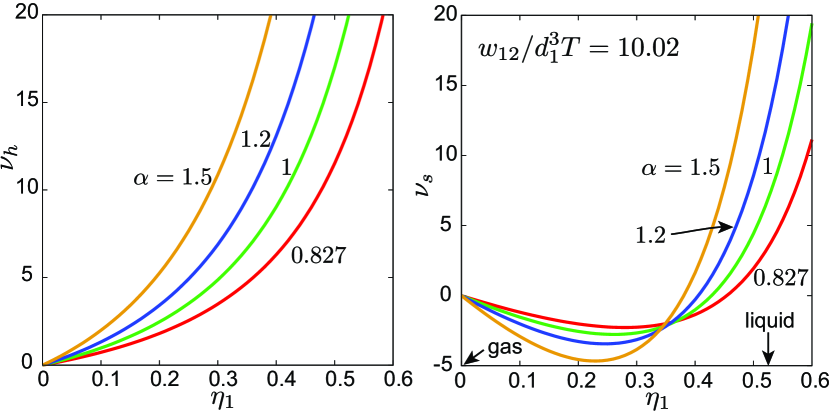
Figure 3: (a) $\nu_{h}$ in Eq.(32) vs solvent volume fraction $\eta_{1}=\pi d_{1}^{3}n_{1}/6$ for four values of size ratio $\alpha$, which is the contribution from repulsive interaction to the solvation chemical potential divided by $T$. Numerical analysis in this paper is performed for $\alpha=0.827$ (lowest curve). (b) Solvation chemical potential $\nu_{s}=\nu_{h}-w_{12}n_{1}/T$ divided by $T$ vs $\eta_{1}$ including attractive interaction in bulk with $w_{12}/d_{1}^{3}T=10.02$. Marked by arrows indicate values of $\eta_{1}$ in two phase coexistence without solute, where $\nu_{s}=3.44$ at this liquid point for $\alpha=0.827$.

We use the symbol $\nu_{s}(n_{1})$ as the solvation chemical potential divided by $T$ in the bulk region:

$$\nu_{s}(n_{1})=\mu_{s}/T=\nu_{h}(n_{1})-w_{12}n_{1}/T.$$ (38)

whose derivative with respect to $n_{1}$ is written as

$$\nu_{s}^{\prime}(n_{1})=\nu_{h}^{\prime}(n_{1})-w_{12}/T.$$ (39)

The pressure $p$ in the bulk region satisfies the thermodynamic relation $p=\sum_{i}n_{i}\mu_{i}-f-\sum w_{ij}n_{i}n_{j}/2$ as in the van der Waals theory. Up to order $n_{2}$ it is written as

$$p=p_{\rm w}(n_{1})+T[1+n_{1}\nu_{s}^{\prime}(n_{1})]n_{2},$$ (40)

where $p_{\rm w}(n_{1})$ is the pressure without solute.

In Fig.3, we plot $\nu_{h}$ and $\nu_{s}$ vs $\eta_{1}=\pi d_{1}^{3}n_{1}/6$ for four values of $\alpha$. We recognize that $\nu_{h}$ increases strongly with increasing $\eta_{1}$ and $\alpha$. In contrast, $\nu_{s}$ in Eq.(38) exhibits a minimum at a density between the gas and liquid densities in the pure fluid limit, $n_{g}$ and $n_{\ell}$. Such a minimum leads to solute adsorption in the gas side of the interface region (see $n_{2}(z)$ in Fig.1). We set $w_{12}=10.02Td_{1}^{3}$ such that $\nu_{s}(n_{\ell})-\nu_{s}(n_{g})\cong\nu_{s}(n_{\ell})$ is equal to $3.44$ (see Eq.(42) below). In our case, we have $n_{\ell}\nu_{s}^{\prime}(n_{\ell})=35.7$, so $\nu_{s}(n_{1})$ is sensitive to small variations of $n_{1}$ and the coefficient of $n_{2}$ in $p$ in Eq.(40) is large in magnitude.

Furthermore, we consider equilibrium gas-liquid coexistence, where the solvent and solute densities in the bulk are $n_{1}^{g}$ and $n_{2}^{g}$ in gas and are ${n}_{1}^{\ell}$ and ${n}_{2}^{\ell}$ in liquid. Tnen, Eq.(37) gives the solute density ratio,

$${{n}_{2}^{\ell}}/n_{2}^{g}=\exp(-\Delta{\nu}_{s})=\exp(-\Delta{\mu}_{s}/T).$$ (41)

Here, $\Delta\mu_{s}=T\Delta{\nu}_{s}$ is the difference of the solvation chemical potential between gas and liquid Ben ; Guillot ; Bu ; Pratt , which is often called the Gibbs transfer free energy (per solute particle in our case). In DFT, Eq.(38) yields

$$\Delta\nu_{s}=[\nu_{h}(n_{1}^{\ell})-\nu_{h}(n_{1}^{g})]-(n_{1}^{\ell}-n_{1}^{g})w_{12}/T.$$ (42)

Note that Eq.(41) is valid even across curved interfaces. If $n_{1}^{\ell}\gg n_{1}^{g}$, we have $\nu_{s}(n_{1}^{g})\cong 0$ and $\Delta\nu_{s}\cong\nu_{s}(n_{1}^{\ell})$. In the dilute limit of solute, we may replace $n_{1}^{g}$ and $n_{1}^{\ell}$ in Eq.(42) by their pure fluid limits, $n_{g}$ and $n_{\ell}$, respectively. Then, the factor $\exp(-\Delta\nu_{s})$ can be related to the Henry constantSander ; Smith , from which $\Delta\nu_{s}$ is $3.44$ for O₂ and is $4.12$ for N₂ in water at $T=300$ Knano . If $\Delta\nu_{s}$ is much larger, the solute tends to form solid aggregates in water as hydrophobic hydration Chandler ; Garde ; Paul .

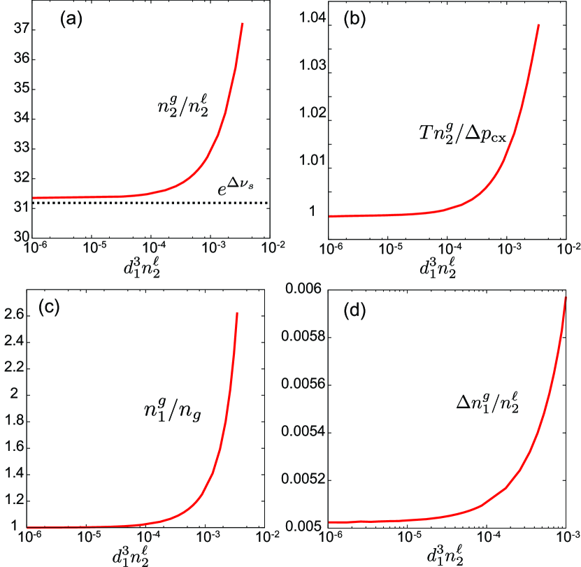
Figure 4: Thermodynamic relations in gas-liquid coexistence in dilute binary mixtures with increasing solute density $n_{2}^{\ell}$ in liquid. (a) Ratio $n_{2}^{g}/n_{2}^{\ell}$ of solute densities in gas and liquid. Its dilute limit is 31, but it increases up to 37 at $d_{1}^{3}n_{2}^{\ell}\sim 0.005$. (b) Ratio $Tn_{2}^{g}/\Delta p_{\rm cx}$ vs $d_{1}^{3}n_{2}^{\ell}$, which is very close to 1 supporting Eq.(53). (c) Ratio $n_{1}^{g}/n_{g}$ vs $d_{1}^{3}n_{2}^{\ell}$, where the pure fluid limit $n_{g}=2.05\times 10^{-5}d_{1}^{-3}$ is very small and $n_{i}^{g}$ remains of order $n_{g}$. (d) Ratio $\Delta n_{1}^{g}/n_{2}^{\ell}$ vs $d_{1}^{3}n_{2}^{\ell}$, where $\Delta n_{1}^{g}=n_{1}^{g}-n_{g}$. It is about 0.005 in accord with Eq.(51).

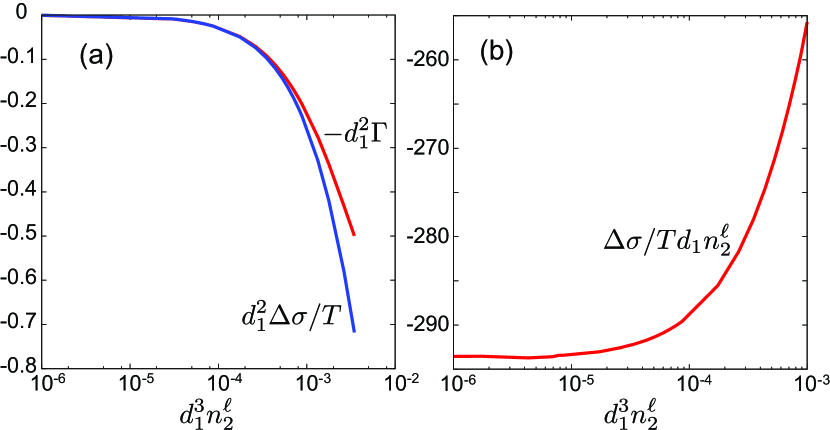
Figure 5: Surface tension change $\Delta\sigma=\sigma-\sigma_{0}$ in dilute mixtures with increasing solute density in liquid $n_{2}^{\ell}$. (a) $d_{1}^{2}\Delta\sigma/T$ vs $d_{1}^{3}n_{2}^{\ell}$, which is compared with normalized surface adsorption of solute $d_{1}^{2}\Gamma$ (see Eq.(57)). (b) Ratio $\Delta\sigma/Td_{1}n_{2}^{\ell}$ vs $d_{1}^{3}n_{2}^{\ell}$, which is about $-290$.

Ishizaki et al. calculated the solvation chemical potential for Lennard-Jones systems via molecular dynamic simulation Koga . We also note that our solvation chemical potential does not account for the effect of orientational degrees of freedom in polar fluids. In particular, for water, we should investigate the effect of the hydrogen bonding on the solvation chemical potential Borgis .

III.2 Algebraic tails in density profiles

We note that the densities themselves have algebraic tails for $|z-z_{\rm int}|\gg d_{1}$ Tara ; Baker ; Hauge , as $\Delta\Pi(z)$ in Eq.(29). For the Lennard-Jones potential in Eq.(7), Eq.(13) gives $\mu_{ai}\cong\sum_{j}w_{ij}n_{j}+TA_{i}(z-z_{\rm int})^{-3}$ with

$$A_{i}={2\pi}\sum_{j}\epsilon_{ij}d_{ij}^{6}(n_{j}^{\ell}-n_{j}^{g})/3T,$$ (43)

Because $\mu_{i}=$const., the deviations defined by $\delta_{\alpha}n_{i}(z)\equiv n_{i}(z)-n_{i}^{\alpha}$ ($\alpha=g,\ell$) decay for $|z-z_{\rm int}|\gg d_{1}$ as

$$\delta_{\alpha}n_{1}(z)/n_{1}^{\alpha}\cong-n_{1}^{\alpha}TK_{\alpha}A_{1}/(z-z_{\rm int})^{3},$$ (44)

$$\delta_{\alpha}n_{2}(z)/n_{2}^{\alpha}\cong-\nu_{s}^{\prime}(n_{1}^{\alpha})\delta_{\alpha}n_{1}-A_{2}/(z-z_{\rm int})^{3}.$$ (45)

In particular, the solute density decays in the gas side as $n_{2}(z)-n_{2}^{g}\sim d_{1}^{6}n_{1}^{\ell}n_{2}^{g}|z-z_{\rm int}|^{-3}$. We have numerically obtained these tails in excellent agreement with Eqs.(42) and (43) (not shown here).

III.3 Thermodynamics in gas-liquid coexistence

When gas and liquid phases are separated by a planar interface, we consider the solute-induced deviations in the bulk. For example, the coexisting (saturated vapor) pressure $p_{\rm cx}$ increases with increasing $n_{2}^{\ell}$ from its pure fluid limit $p_{\rm cx}^{0}$, where $p_{\rm cx}^{0}=2.1\times 10^{-5}p_{0}$ with $p_{0}=Td_{1}^{-3}$ in our case. To linear order in $n_{2}^{\alpha}$, the deviation of $\mu_{1}$ and the shift $\Delta p_{\rm cx}=p_{\rm cx}-p_{\rm cx}^{0}$ are calculated as Onuki1

$$\Delta\mu_{1} = (n_{\alpha}^{2}K_{\alpha})^{-1}\Delta n_{1}^{\alpha}+T\nu_{s}^{\prime}(n_{\alpha})n_{2}^{\alpha},$$ (46)

$$\Delta p_{\rm cx} = (n_{\alpha}K_{\alpha})^{-1}\Delta n_{1}^{\alpha}+T[1+n_{\alpha}\nu_{s}^{\prime}(n_{\alpha})]n_{2}^{\alpha}$$ (47)

$$= n_{\alpha}\Delta\mu_{1}+Tn_{2}^{\alpha},$$

where $\Delta n_{1}^{\alpha}=n_{1}^{\alpha}-n_{\alpha}$ is the solvent density deviation and $K_{\alpha}$ is the isothermal compressibility of pure solvent in phase $\alpha$ defined by $f_{w}^{\prime\prime}(n_{\alpha})-w_{11}=1/n_{\alpha}^{2}K_{\alpha}$. These relations hold both for gas and liquid $(\alpha=g,\ell)$. Thus,

$$\Delta\mu_{1}=-T[n_{2}]/[n_{1}]=T(n_{2}^{g}-n_{2}^{\ell})/(n_{\ell}-n_{g}),$$ (48)

$$\Delta n_{1}^{\alpha}=-Tn_{\alpha}^{2}K_{\alpha}([n_{2}]/[n_{1}]+\nu_{s}^{\prime}(n_{\alpha})n_{2}^{\alpha}).$$ (49)

Here, for any quantity ${\cal A}$, the difference of the values of ${\cal A}$ in coexisting liquid and gas is written as $[{\cal A}]={\cal A}_{\ell}-{\cal A}_{g}$. For example, $[n_{i}]=n_{i}^{\ell}-n_{i}^{g}$. Dividing the second line of Eq.(47) by $n_{\alpha}$, we also obtain the solute-induced shift of the coexisting pressure.Onuki1 ,

$$\Delta p_{\rm cx}=T\frac{[n_{2}/n_{1}]}{[1/n_{1}]}=T\frac{n_{\ell}n_{2}^{g}-n_{g}n_{2}^{\ell}}{n_{\ell}-n_{g}}.$$ (50)

In our previous paper nano we assumed the conditions $n_{\ell}\gg n_{g}$ and $\exp(\Delta\nu_{s})\gg 1$ far from the criticality, where Eqs.(49) and (50) are rewritten as

$${\Delta n_{1}^{g}}\cong[1-n_{\ell}\nu_{s}^{\prime}(n_{g})]({n_{g}}/{n_{\ell}})n_{2}^{g},$$ (51)

$${\Delta n_{1}^{\ell}}\cong{Tn_{\ell}K_{\ell}}[1-e^{-\Delta\nu_{s}}n_{\ell}\nu_{s}^{\prime}(n_{\ell})]{n_{2}^{g}},$$ (52)

$$\Delta p_{\rm cx}\cong Tn_{2}^{g}=e^{\Delta\nu_{s}}Tn_{2}^{\ell},$$ (53)

Here, $\Delta n_{1}^{g}$ is much smaller than $n_{2}^{g}$ by the factor ${n_{g}}/{n_{\ell}}$ in Eq.(51) and the pressure shift $p_{\rm cx}$ arises solely from the solute in gas for $n_{2}^{g}\gg n_{1}^{g}$ in Eq.(53). Also $\Delta n_{1}^{\ell}$ can be very small for sufficiently small $K_{\ell}\ll 1/n_{\ell}T$. In our analysis, we obtain $Tn_{\ell}K_{\ell}=0.025$, $n_{\ell}\nu_{s}^{\prime}(n_{g})=-7.07$, $n_{\ell}\nu_{s}^{\prime}(n_{\ell})=35.7$, and $e^{-\Delta\nu_{s}}n_{\ell}\nu_{s}^{\prime}(n_{\ell})=1.14$. Substitution of these values in Eqs.(51) and (52) yields $\Delta n_{1}^{g}\cong 1.6\times 10^{-4}n_{2}^{g}$ and $\Delta n_{1}^{\ell}\cong-3.6\times 10^{-3}n_{2}^{g}$. Thus, the solvent density is almost unchanged both in gas and liquid.

In Fig.4, we plot the ratios (a) $n_{2}^{g}/n_{2}^{\ell}$, (b) $Tn_{2}^{g}/\Delta p_{\rm cx}$, (c) $n_{1}^{g}/n_{g}$, and (d) $\Delta n_{1}^{g}/n_{2}^{\ell}$ as functions of $n_{2}^{\ell}$. In (a), the density ratio obeys Eq.(41) with $\Delta\nu_{s}=3.44$ for $d_{1}^{3}n_{2}^{\ell}\lesssim 10^{-3}$, but it increases up to 37 for larger $n_{2}^{\ell}$. In (b), Eq.(53) holds for all $n_{2}^{\ell}$ investigated. In (c), $n_{1}^{g}/n_{g}$ increases from 1 up to about 2.6 staying at very small values. In (d), $\Delta n_{1}^{g}$ increases with increasing $n_{2}^{\ell}$ linearly as $\Delta n_{1}^{g}\cong 0.005n_{2}^{\ell}\cong 1.6\times 10^{-3}n_{2}^{g}$ in accord with Eq.(51).

We note that Eqs.(46)-(53) are general thermodynamic relations. Let us consider the Gibbs-Duhem relation of binary mixtures at fixed $T$ in two-phase coexistence,

$$dp=n_{1}^{\alpha}d\mu_{1}+n_{2}^{\alpha}d\mu_{2},$$ (54)

which holds both for $\alpha=g$ and $\ell$. Since $n_{2}d\mu_{2}\cong Tdn_{2}$ for small $n_{2}$, integration of Eq.(54) with respect to $n_{2}$ yields Eqs.(47)-(50).

With addition of a solute, a homogeneous liquid (without bubbles) becomes metastable against bubble formation if its pressure $\bar{p}$ is made slightly lower than $p_{\rm cx}=p_{\rm cx}^{0}+\Delta p_{\rm cx}$. This condition can be realized even outside the solvent coexistence curve ${\bar{p}}>p_{cx}^{0}$ if $n_{2}^{\ell}$ exceeds a threshold solute density $n_{2}^{c}$ nano given by

$$n_{2}^{c}=e^{-\Delta\nu_{s}}({\bar{p}}-p_{\rm cx}^{0})/T.$$ (55)

For ${\bar{p}}<p_{cx}^{0}$ (inside CX), bubbles can appear even without solute, so we may set $n_{2}^{c}=0$. In ambient water with ${\bar{p}}-p_{\rm cx}^{0}\sim 1$ atm, $n_{2}^{c}$ is very small even for mildly hydrophobic gases such as O₂ and N₂nano .

We also examine the deviation of the surface tension $\Delta\sigma=\sigma-\sigma_{0}$ due to dilute solute, where $\sigma_{0}$ is the surface tension without solute. We consider the deviation of $\omega$ in Eq.(19), where the coefficient in front of the solute density deviation $\Delta n_{1}(z)$ vanishes from the homogeneity of $\mu_{1}$ Onuki1 . To first order in $n_{2}$, we find

$$\Delta\sigma=\int dz[\Delta p_{\rm cx}-n_{1}(z)\Delta\mu_{1}-Tn_{2}(z)].$$ (56)

From Eqs.(48) and (50), we obtain the Gibbs adsorption formula $\Delta\sigma=-T\Gamma$ Gibbs . Here, $\Gamma$ is the solute adsorption,

$$\Gamma=\int dz\bigg{[}n_{2}(z)-n_{2}^{g}-\frac{[n_{2}]}{[n_{1}]}(n_{1}(z)-n_{1}^{g})\bigg{]}.$$ (57)

In Fig.1, we notice that the adsorption occurs in the gas side in (b) and (c) of Fig.1 (left of the Gibbs dividing surface), where $\Gamma=0.132d_{1}^{-2}$ in (b) and $\Gamma=0.432d_{1}^{-2}$ in (c). Furthermore, in Fig.5, we plot (a) $\Delta\sigma$ and $\Gamma$ and (b) $\Delta\sigma/n_{2}^{\ell}$ as functions of $n_{2}^{\ell}$. In addition to the Gibbs adsorption law, we can see the linear behavior $-\Delta\sigma/d_{1}T\cong 290n_{2}^{\ell}\cong 9.3n_{2}^{g}$ for small $n_{2}^{\ell}$.

In our previous thermodynamic theorynano , we assumed a constant $\sigma$ independent of the solute density. However, a decrease in $\sigma$ increases the stability of small bubbles with a smaller Laplace pressure. The Gibbs law has been used for interfacial adsorption of neutral surfactants. Its generalization including the electrostatic interaction was given in our previous papersBu ; Onukisurf .

III.4 Stable solute-induced bubbles

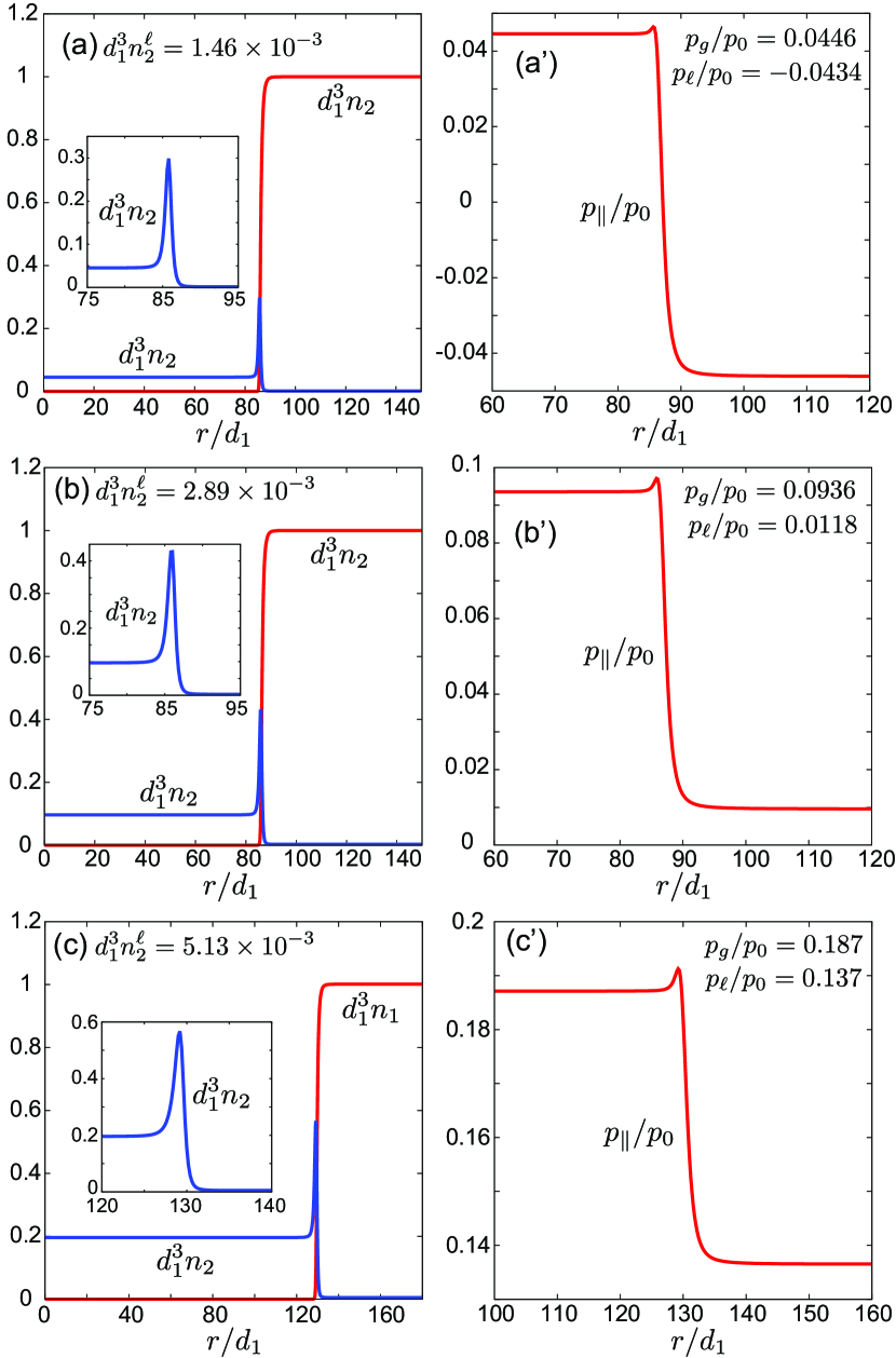
Figure 6: Densities $n_{1}(r)$ and $n_{2}(r)$ (left) and pressure $p_{\parallel}(r)$ along $\hat{\mbox{\boldmath$r$}}$ (right) around stable spherical bubbles, where $d_{1}^{3}n_{2}^{\ell}$ is (a) $1.46\times 10^{-3}$, (b) $2.89\times 10^{-3}$, (c) $5.13\times 10^{-3}$, with $d_{1}^{3}n_{1}^{\ell}\cong 1$. Pressures $(p_{g},p_{\ell})$ in bulk gas and liquid are (a) $(0.0446,-0.0434)$, (b) $(0.0936,0.0118)$, and (c) $(0.187,0.137)$ in units of $p_{0}=T/d_{1}^{3}=153$ MPa, where the difference $p_{g}-p_{\ell}$ is close to $2\sigma/R$. Here, $p_{\ell}$ is negative ($-6$ Mpa) in (a), while it is much above $p_{\rm cx}^{0}$ for (b) and (c). Cell length $L$ is $400d_{1}$ in (a) and (b) and is $800d_{1}$ in (c).

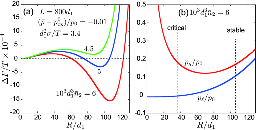
Figure 7: (a) Bubble free energy $\Delta F$ in Eq.(65) vs $R$ at fixed volume with $L=800d_{1}$, where initial pressure is ${\bar{p}}=p_{cx}^{0}-0.01Td_{1}^{-3}$. Initial solute density is ${\bar{n}}_{2}=4.5,5$, and $6$ in units of $10^{-3}d_{1}^{-3}$ for three curves. A stable bubble is realized for the lower two curves at the minimum radius $R_{m}$. (b) Pressures inside and outside bubble $p_{g}$ and $p_{\ell}$ in Eq.(65) for the lowest curve in (a). Vertical broken lines indicate critical and stable bubble radii, $R_{c}=37.2d_{1}$ and $R_{m}=106.6d_{1}$.

In our previous papernano , we showed that small, stable bubbles minimize an appropriately defined bubble free energy for ${\bar{p}}>p_{\rm cx}^{0}$. They are induced by a small amount of moderately hydrophobic gas in water. In contrast, in pure fluids, equilibrium bubbles with macroscopic sizes appear at fixed cell volume inside CX Onukibook ; Binder . Here, we place a spherical bubble at the center of a spherical cell, fixing the total solvent and solute numbers $N_{1}$ and $N_{2}$. See Fig.6 for typical density profiles around stable bubbles.

III.4.1 Stress tensor around a bubble and Laplace law

In our spherically symmetric geometry, we take the reference frame with the origin at the bubble center. The average stress tensor is generally of the formOno ; Scho ,

$${\Pi_{\alpha\beta}}=p_{\parallel}(r)\delta_{\alpha\beta}-\Delta\Pi(r)(\delta_{\alpha\beta}-{\hat{x}}_{\alpha}\hat{x}_{\beta}),$$ (58)

where ${\hat{\mbox{\boldmath$r$}}}=(\hat{x},\hat{y},\hat{z})=r^{-1}{\mbox{\boldmath$r$}}$. The parallel component $p_{\parallel}(r)=\sum_{\alpha\beta}{\Pi_{\alpha\beta}}\hat{x}_{\alpha}\hat{x}_{\beta}$ and the stress difference $\Delta\Pi(r)$ depend only on $r$. With Eq.(58), the mechanical equilibrium condition $\sum_{\beta}\nabla_{\beta}{\Pi_{\alpha\beta}}=0$ is rewritten as

$$\frac{d}{dr}p_{\parallel}(r)=-\frac{2}{r}\Delta\Pi(r).$$ (59)

We assume that the bubble radius $R$ much exceeds the molecular lengths, where it is determined by

$$R=\int_{0}^{L}dr[n_{1}(r)-n_{1}^{\ell}]/[n_{1}^{g}-n_{1}^{\ell}].$$ (60)

We first calculate $\Delta\Pi(r)$ for $R\gg d_{1}$. Since $2\Delta\Pi=3\sum_{\alpha\beta}\Pi_{\alpha\beta}{\hat{x}}_{\alpha}\hat{x}_{\beta}-\sum_{\alpha}\Pi_{\alpha\alpha}$ from Eq.(58), Eq.(10) yields

$$\Delta\Pi(r)=\frac{1}{4}\int d{\mbox{\boldmath$r$}}_{1}\int d{\mbox{\boldmath$r$}}_{2}\sum_{ij}[r_{12}-{3}(\hat{\mbox{\boldmath$r$}}\cdot{{\mbox{\boldmath$r$}}}_{12})^{2}/r_{12}]$$

$$\hskip 11.38109pt\times\phi^{\prime}_{ij}(r_{12})\delta_{s}({\mbox{\boldmath$r$}},{\mbox{\boldmath$r$}}_{1},{\mbox{\boldmath$r$}}_{2})n_{i}({r}_{1})n_{j}({r}_{2}),$$ (61)

where the integrand is nonvanishing only for $r_{1}<r<r_{2}$ or $r_{2}<r<r_{1}$ due to the $\delta_{s}$ function. Furthermore, if we set $u=r_{12}=|{\mbox{\boldmath$r$}}_{1}-{\mbox{\boldmath$r$}}_{2}|$, the integrand is also nonvanishing only for $|r_{1}-r_{2}|<u<r_{1}+r_{2}$. Under these conditions of $r_{1}$ and $r_{2}$, the angle integration in Eq.(61) can be performed with the aid of the relation,

$$\int d\Omega_{1}\int d\Omega_{2}\delta(r_{12}-u)\delta_{s}({\mbox{\boldmath$r$}},{\mbox{\boldmath$r$}}_{1},{\mbox{\boldmath$r$}}_{2})=\frac{4\pi u}{rr_{1}r_{2}{W}},$$ (62)

where $d\Omega_{i}$ ($i=1,2)$ are the solid angle elements in $d{\mbox{\boldmath$r$}}_{i}=dr_{i}r_{i}^{2}d\Omega_{i}$ and $W^{2}=u^{4}-2u^{2}(r_{1}^{2}+r_{2}^{2}-2r^{2})+(r_{1}^{2}-r_{2}^{2})^{2}$. For $r\gg d_{1}$, we may set $\hat{\mbox{\boldmath$r$}}\cdot{{\mbox{\boldmath$r$}}}_{12}\cong r_{1}-r_{2}$ in Eq.(61) and $W\cong 2r|r_{1}-r_{2}|$ in Eq.(62) to find

$$\Delta\Pi\cong\int_{z}^{L}dr_{1}\int_{0}^{z}dr_{2}\sum_{ij}\frac{\Theta_{ij}(r_{1}-r_{2})}{r_{1}-r_{2}}n_{i}(r_{1})n_{j}(r_{2}),$$ (63)

which is of the same form as $\Delta\Pi(z)$ in Eq.(27). Thus, $\Delta\Pi(r)$ behaves in the same manner as $\Delta\Pi(z)$ and its $r$-integral is equal to the surface tension $\sigma$ with a correction of order $R^{-1}$. The Laplace law then follows if Eq.(59) is integrated across the interface at $r\cong R\gg d_{1}$.

In Fig.6, we display $n_{1}(r)$, $n_{2}(r)$, and $p_{\parallel}(r)$ around stable spherical bubbles, where we calculate the densities with the method in Appendix C and $p_{\parallel}(r)$ from Eqs.(59) and (63). Here, $d_{1}^{3}n_{2}^{\ell}$ is (a) $1.46\times 10^{-3}$, (b) $2.89\times 10^{-3}$, and (c) $5.13\times 10^{-3}$, while $d_{1}^{3}n_{1}^{\ell}\cong 1$. The cell radius $L$ is 400 in (a) and (b) and is 800 in (c). Remarkably, the liquid pressure $p_{\ell}$ is negative at $-0.0434p_{0}=-6$ MPa in (a), while $p_{\ell}/p_{0}$ is $0.0118$ in (b) and 0.196 in (c). A small peak of $p_{\parallel}$ at the interface in (b) and (c) is due to the solute adsorption. Then, $R/d_{1}$ is (a) 86.3, (b) 86.5, and (c) 129.8, while $d_{1}^{2}\sigma/T$ is (a) 3.67, (b) 3.40, and (c) 3.06 from the integral of $\Delta\Pi$ in Eq.(63). These values yield the normalized Laplace pressure $2\sigma/Rp_{0}$ as (a) $0.0851$, (b) $0.0786$, and (c) $0.0471$, in good agreement with the normalized pressure difference $(p_{g}-p_{\ell})/p_{0}$ given by (a) $0.088$, (b) $0.082$, (c) $0.050$, where $p_{0}=Td_{1}^{-3}=153$ MPa.

Using DFT, Talanquer et al.Ox calculated the density profiles of unstable critical bubbles at $R=R_{c}$, where the solute is accumulated in the bubble interior and its density exhibits a mild maximum at the interface. In their molecular dynamics simulation, Yamamoto and Ohnishi Yama realized stable helium-rich nanobubbles in water. They fixed the cell volume to find slightly negative pressures in the liquid region as in our Fig.6(a).

III.4.2 Equilibrium conditions and critical radius

We start with a reference (metastable) liquid state without bubbles, where the densities are ${\bar{n}}_{i}=N_{i}/V$ and the pressure is $\bar{p}$. With appearance of a single bubble at fixed cell volume, the densities in liquid are changed as

$$n_{1}^{\ell} = (1+\phi){\bar{n}}_{1},$$ (64)

$$n_{2}^{\ell} = {\bar{n}}_{2}-\phi n_{2}^{g},$$ (65)

where $\phi=4\pi R^{3}/3V$ is the bubble volume fraction. Here, we assume $\phi<{\bar{n}}_{2}/n_{2}^{g}\ll 1$. We also neglect small density heterogeneities around the bubble when it is growing or shrinking. Using the liquid compressibility $K_{\ell}$, we write the pressures in liquid and gas as

$$p_{\ell} = {\bar{p}}+\phi/K_{\ell},$$ (66)

$$p_{g} = {\bar{p}}+\phi/K_{\ell}+2\sigma/R.$$ (67)

In $p_{\ell}$ we neglect the second term ($\propto n_{2}$) in Eq.(40), which is allowable for $n_{2}^{g}/n_{\ell}\ll[Tn_{\ell}K_{\ell}(1+n_{\ell}\nu_{s}^{\prime}(n_{\ell})]^{-1}\cong 1$. For small $K_{\ell}$, the compression pressure $\phi/K_{\ell}$ can be significant even for small $\phi$. For $p_{g}>p_{\rm cx}^{0}$, the solvent density in gas $n_{1}^{g}$ is almost unchanged from $n_{g}=p_{\rm cx}^{0}/T$. The gas pressure is also given by $p_{g}=T(n_{1}^{g}+n_{2}^{g})$, so

$$n_{2}^{g}=({\bar{p}}-p_{\rm cx}^{0}+2\sigma/R+\phi/K_{\ell})/T.$$ (68)

If ${\bar{p}}<p_{\rm cx}^{0}$, we require $p_{\rm cx}^{0}-{\bar{p}}<(8/3)(2\pi\sigma^{3}/K_{\ell}V)^{1/4}=31.4Td_{1}^{-9/4}V^{-1/4}$ to ensure $n_{2}^{g}>0$.

If we further assume the chemical balance in Eq.(41), $n_{2}^{g}$ is also expressed as

$$n_{2}^{g}={\bar{n}}_{2}/[e^{-\Delta\nu_{s}}+\phi].$$ (69)

For given ${\bar{n}}_{2}$ and $\bar{p}$, Eqs.(68) and (69) constitute a closed set of equations of $R$. Previously nano , we solved them without $\phi/K_{\ell}$ at fixed ${\bar{p}}$ in liquid. Also in the present fixed-volume case, we obtain two solutions at $R=R_{c}$ and $R_{m}$ for sufficiently large ${\bar{n}}_{2}$, as in Fig.7(a). The larger one $R_{m}$ is the radius of a stable or metastable bubble, while the smaller one $R_{c}$ is the critical radius of an unstable bubble. In the limit $\phi\to 0$, $R_{c}$ is written as

$$R_{c} = 2\sigma/[T{\bar{n}}_{2}e^{\Delta\nu_{s}}-{\bar{p}}+p_{\rm cx}^{0}]$$ (70)

$$= 2\sigma e^{-\Delta\nu_{s}}/T({\bar{n}}_{2}-n_{2}^{c}),$$

where $n_{2}^{c}$ is the threshold solute density in Eq.(55). Thus, solute-induced metastability is realized for ${\bar{n}}_{2}>n_{2}^{c}$. For pure fluids, $R_{c}=2\sigma/(p_{\rm cx}^{0}-{\bar{p}})$ inside CX Katz . Azouzi et al. Caupin performed a nucleation experiment at negative pressures about $-100$ MPa.

III.4.3 Bubble free energy at fixed $N_{1}$-$N_{2}$-$V$-$T$

We set up a bubble free energy $F_{b}$, removing the solvent degrees of freedom. At fixed $V$, it is the change of the Helmholtz free energy with appearance a single bubble. Using Eqs.(64) and (66), we express it as nano

$$F_{b}=V(\phi\omega_{g}+\omega_{\ell})+S\sigma,$$ (71)

where $S=4\pi R^{2}$, $\phi=4\pi R^{3}/3V\ll 1$, and

$$\omega_{g} = Tn_{2}^{g}[\ln({n_{2}^{g}/{\bar{n}}_{2}})-1-{\Delta{\nu}_{s}}]+{\bar{p}}-p^{0}_{\rm cx},$$ (72)

$${\omega}_{\ell} = T[{n}_{2}^{\ell}\ln({n}_{2}^{\ell}/{{\bar{n}}_{2}})+\phi n_{2}^{g}]+\phi^{2}/2K_{\ell}.$$ (73)

Here, we assume Eq.(65); then, $F_{b}$ depends on $n_{2}^{g}$ and $\phi$. Against infinitesimal changes $n_{2}^{g}\to n_{2}^{g}+\delta n_{2}^{g}$ and $\phi\to\phi+\delta\phi$, the incremental change in $\Delta F$ is written as

$${\delta F_{b}} = VT[\ln({n_{2}^{g}}/{{n}_{2}^{\ell}})-\Delta\nu_{\rm s}]\delta(n_{2}^{g}\phi)$$ (74)

$$+V[{p_{g}-p_{\rm cx}^{0}}-Tn_{2}^{g}]\delta\phi.$$

in terms of $p_{g}$ in Eq.(67). In equilibrium, $F_{b}$ is minimized with respect to $n_{2}^{g}$ and $\phi$, leading to Eqs.(44) and (68).

Let us assume the mechanical equilibrium condition (68) and not the chemical one (44). Note that the former is instantaneously realized in the slow nucleation process. Then, $F_{b}$ is a function of $R$ and its derivative is given by

$$\frac{1}{S}\frac{dF_{b}}{dR}=\bigg{[}\ln\frac{n_{2}^{g}}{{n}_{2}^{\ell}}-\Delta\nu_{\rm s}\bigg{]}\bigg{[}{\bar{p}}-p_{\rm cx}^{0}+\frac{4\sigma}{3R}+\frac{4\phi}{3K_{\ell}}\bigg{]},$$ (75)

which vanishes under Eq.(41). For sufficiently large ${\bar{n}}_{2}$, $F_{b}(R)$ exhibits a local maximum at $R=R_{c}$ and a local minimum at $R=R_{m}(>R_{c})$. Here, $R_{c}$ is the critical radius expressed as in Eq.(70) in the limit $\phi\to 0$, while $R_{m}$ is a stable (metastable) bubble radius for negative (positive) $F_{b}(R_{m})$.

In Fig.7(a), we plot $F_{b}(R)$ in Eq.(71) vs $R$ at $L=800d_{1}$, where ${\bar{n}}_{1}\cong 1$ and ${\bar{n}}_{2}=4.5$, $5$, and $6$ in units of $10^{-3}d_{1}^{-3}$ for the three curves. The initial pressure is ${\bar{p}}=p_{cx}^{0}-0.01p_{0}$. In Fig.7(b), we plot the pressures $p_{\ell}$ and $p_{g}$ in Eqs.(66) and (67) vs $R$ for the curve of the largest ${\bar{n}}_{2}$ in (a). The density profiles for the stable bubble in this case are close to those in Fig.6(c).

IV Dynamics of a solute-induced bubble

Finally, we examine bubble dynamics combining DFT and hydrodynamics. In this paper, we assume homogeneous $T$ in the limit of fast heat conduction. This approximation is allowable for slow solute diffusionnano . However, $T$ becomes inhomogeneous around growing or shrinking bubbles firstly due to adiabatic heating or cooling of bubbles and secondly due to latent heat in evaporation and condensation Szeri ; Plesset ; Nepp ; Teshi ; Teshi1 ; Teshi2 . We should examine these effects in future simulations.

IV.1 Hydrodynamic equations

We consider the mass densities $\rho_{i}=m_{i}n_{i}$, the velocity field $v$, and the momentum density ${\mbox{\boldmath$J$}}=\rho{\mbox{\boldmath$v$}}$, where $m_{1}$ and $m_{2}$ are the molecular masses and $\rho=\rho_{1}+\rho_{2}$ is the total mass density. The mass conservation yields Landau

$$\frac{\partial\rho_{1}}{\partial t}=-\nabla(\rho_{1}{\mbox{\boldmath$v$}}-{\mbox{\boldmath$I$}}),$$ (76)

$$\frac{\partial\rho_{2}}{\partial t}=-\nabla(\rho_{2}{\mbox{\boldmath$v$}}+{\mbox{\boldmath$I$}}),$$ (77)

where $I$ is the diffusion flux of the form,

$${\mbox{\boldmath$I$}}=-\Lambda\nabla(\mu_{2}/m_{2}-\mu_{1}/m_{1}).$$ (78)

If the solute is dilute or $n_{2}$ is small, the kinetic coefficient $\Lambda$ is related to the solute diffusion constant $D$ by

$$\Lambda=Dm_{2}^{2}n_{2}/T.$$ (79)

Then, as $n_{2}\to 0$, we have $\nabla\rho_{2}\cong Tn_{2}^{-1}\nabla n_{2}$ and ${\mbox{\boldmath$I$}}\cong-D\nabla\rho_{2}$. Next, the momentum equation is written as

$$\frac{\partial{\mbox{\boldmath$J$}}}{\partial t}+\nabla\cdot[\rho{\mbox{\boldmath$v$}}{\mbox{\boldmath$v$}}]=-\nabla\cdot(\tensor{\Pi}-{\tensor{\sigma}}_{\rm vis})-\sum_{i}n_{i}\nabla U_{i}$$

$$\hskip 39.83368pt=-\sum_{i}n_{i}\nabla\mu_{i}+\nabla\cdot{\tensor{\sigma}}_{\rm vis}.$$ (80)

Here, $\tensor{\Pi}=\{\Pi_{\alpha\beta}\}$ is the stress tensor in Eq.(10) determined by $n_{i}$, and $U_{i}$ is the wall potential. The second line follows from Eq.(12). The $\tensor{\sigma}_{\rm vis}=\{\sigma_{\alpha\beta}\}$ is the viscous stress tensor of the form,

$$\sigma_{\alpha\beta}={\eta}_{s}(\nabla_{\alpha}v_{\beta}+\nabla_{\beta}v_{\alpha})+(\eta_{b}-2{\eta}_{s}/3)(\nabla\cdot{\mbox{\boldmath$v$}})\delta_{\alpha\beta},$$ (81)

where $\eta_{s}$ is the shear viscosity and $\eta_{b}$ is the bulk viscosity. In the previous papers on dynamical DFT Lowen ; Lutsko ; Goddard ; Donev , the shear viscosity was introduced to include the hydrodynamic interaction among colloidal particles.

The total free energy ${\cal F}_{\rm tot}={\cal F}+{\cal K}$ is the sum of the Helmholtz free energy functional ${\cal F}$ and the fluid kinetic energy $\cal K$. The latter is written as

$${\cal K}=\frac{1}{2}\int d{\mbox{\boldmath$r$}}\rho v^{2}.$$ (82)

If the total particle numbers $N_{i}=\int d{\mbox{\boldmath$r$}}n_{i}$ are fixed and $v$ vanishes on the boundaries, our dynamic equations yield

$$\frac{d}{dt}{\cal F}_{\rm tot}=-\int d{\mbox{\boldmath$r$}}\bigg{[}\Lambda^{-1}|{\mbox{\boldmath$I$}}|^{2}+\sum_{\alpha,\beta}\sigma_{\alpha\beta}\nabla_{\alpha}v_{\beta}\bigg{]}\leq 0.$$ (83)

Thus, at long times, a stationary state should be realized with $\nabla\mu_{1}=\nabla\mu_{2}={\mbox{\boldmath$v$}}={\mbox{\boldmath$0$}}$.

In the kinetic theory of dilute gases, $\eta_{s}$ tends a small constant of order $(m_{1}T)^{1/2}d_{1}^{-2}$ and $\eta_{b}$ tends to zero in the dilute limit Hir . These density-dependences have been confirmed in molecular dynamics simulations Hasse ; shear ; bulk . In our case, they are crucial for the hydrodynamics in bubble. Thus, we used simple extrapolation forms,

$${\eta_{s}}/{\eta_{0}}=0.14+0.86d_{1}^{3}n,$$ (84)

$${\eta_{b}}/{\eta_{0}}=(0.02+0.98d_{1}^{3}n)d_{1}^{3}n,$$ (85)

where $n=n_{1}+n_{2}$ and $\eta_{0}$ is the viscosity in liquid.

IV.2 Numerical results after liquid decompression

IV.2.1 Method

We solved the above dynamic equations in a spherical cell with radius $L=200d_{1}$, where $v$ and $I$ are parallel to ${\hat{\mbox{\boldmath$r$}}}=r^{-1}{\mbox{\boldmath$r$}}$, so we may set

$${\mbox{\boldmath$v$}}=v(r,t){\hat{\mbox{\boldmath$r$}}},\quad{\mbox{\boldmath$I$}}=I(r,t){\hat{\mbox{\boldmath$r$}}}.$$ (86)

As the boundary condition, we assumed $v(L,t)=I(L,t)=0$ to fix the total particle numbers in the cell. The mesh length in time integration was $0.2d_{1}$.

Together with the parameters in Eq.(8), we assumed $m_{1}=3\times 10^{-23}$ g, $m_{2}=(16/9)m_{1}$, $D=2\times 10^{-4}$ cm${}^{2}/$s, and $\eta_{0}=0.89$ cP. Using $\eta_{0}$ in Eqs.(84) and (85), we measure time in units of

$$\tau=m_{1}/d_{1}\eta_{0}=0.112~{}{\rm ps}.$$ (87)

Then, we have $(d_{1}^{2}m_{1}/\epsilon_{11})^{1/2}=0.041\tau$ as a characteristic microscopic time and $R^{2}/D=4.0\times 10^{6}\tau$ as a typical diffusion time around a bubble with radius $R=30$ nm. The wall potential was assumed to be attractive as ${U_{1}}=-6.5T\exp(-{s}/{1.4})$ and ${U_{2}}=-0.5T\exp(-{s}/{1.23})$ with $s=(L-r)/d_{1}$, where $L=200d_{1}$ is the cell radius. Then, the wall prefers the solvent more than the solute and no surface bubble appears.

For $t<0$, we prepared a stable bubble with radius $R_{\rm ini}=53.11d_{1}$ with the initial densities $n_{1}^{g}=8.37\times 10^{-5}$, $n_{1}^{\ell}=1.00$, $n_{2}^{g}=0.207$, and $n_{2}^{\ell}=5.68\times 10^{-3}$ in units of $d_{1}^{-3}$. At $t=0$, we suddenly decreased the liquid density $n_{1}^{\ell}$ in the region $r>R_{\rm ini}$ to $0.900d_{1}^{-3}$, which gave rise to a negative liquid pressure about $-2.73p_{0}=-419$ MPa (in a very short time). Then, the bubble expanded exhibiting a damped oscillation. At $t=5000\tau$, the bubble radius became close to the final radius $R_{\infty}=98.52d_{1}$, but the solute density in gas $n_{2}^{g}$ was $0.040d_{1}^{-3}$ and was still noticeably smaller than the final value $0.060d_{1}^{-3}$. Note that the final equilibrium state can be realized with the method in Appendix C.

Our initial condition and the isothermal assumption are rather unrealistic, but the resultant dynamical processes are dramatic, providing fundamental information on the nonlinear bubble dynamics in confined geometries.

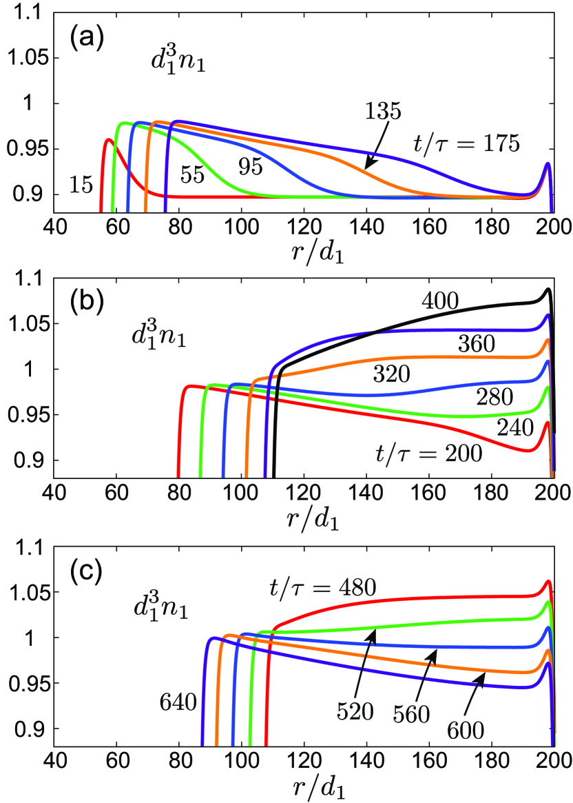
Figure 8: Time-evolution of solvent density $n_{1}(r,t)$ outside a bubble with time-dependent radius $R(t)$ after decompression of liquid in a cell with $L=200$. (a) The bubble expands emitting a large-amplitude sound outward. (b) Stepwise sound reaches the cell boundary, while the bubble is still expanding. (c) The bubble is shrinking, which causes a large decrease of $n_{1}(r,t)$ in liquid.

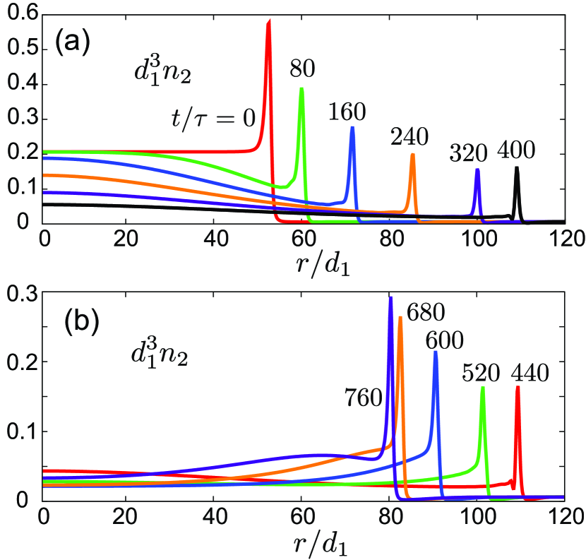
Figure 9: Time-evolution of solute density $n_{2}(r,t)$ inside a bubble during its expansion in (a) and its shrinkage in (b). Outward and inward interface motions propagate as acoustic waves. The sound speed is of the same order as the interface velocity. In (b), scale of the vertical axis is twice enlarged.

IV.2.2 Acoustic disturbances

In Fig.8, we show the profiles of the solvent density $n_{1}(r,t)$ outside the oscillating bubble at consecutive times. In (a), a large-amplitude acoustic wave is emitted in a stepwise form from the bubble surface. Its expanding speed is given by the (isothermal) sound velocity $c_{\ell}=\sqrt{(\partial p/\partial\rho)_{T}}=0.88d_{1}/\tau$, which is larger than the maximum bubble expanding speed about $0.2(d_{1}/\tau)$. Its amplitude is gradually decreases away from the bubble, being proportional to $r^{-1}$ in this spherically symmetric geometry. In (b), the wave reaches the cell boundary and $n_{1}$ increases near the wall. In (c), the bubble shrinks, causing an overall density decrease in the liquid region.

In Fig.9, we also show the profiles of the solute density $n_{2}(r,t)$ at consecutive times, which is appreciable in the bubble and has an adsorption peak. The solvent density $n_{1}(r,t)$ remains of order $10^{-5}-10^{-4}d_{1}^{-3}$ in the bubble. In (a), the outward interface motion gives rise to a negative stepwise wave propagating inward with the sound speed $c_{g}=(T/m_{2})^{1/2}=0.14d_{1}/\tau$. Here, the acoustic traversal time $R/c_{g}$ is about $880\tau$ and is close to the oscillation period $650\tau$. In (b), $n_{2}(r,t)$ still changes inhomogeneously during the bubble shrinkage. However, it becomes gradually homogeneous after several oscillations. If we would use liquid viscosities in the bubble, we would have uniform dilation with $v_{i}\propto x_{i}$ from the early stage. It is worth noting that the bubble interior has been assumed to be homogeneous in the literature Plesset ; Nepp ; Szeri ; sonol . In addition, we notice that the adsorption $\Gamma$ in our case noticeably depends on time (see Fig.13(d) and its explanation).

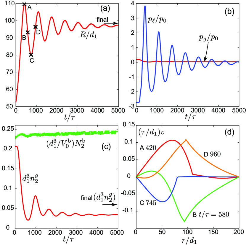
Figure 10: Earlt-stage time-evolution ($0<t<5000\tau$). (a) Bubble radius $R(t)$, which approaches the final radius (arrow). (b) Liquid pressure $p_{\ell}(t)$ at $r=170d_{1}$ and gas pressure $p_{g}(t)$ at $r=2d_{1}$ divided by $p_{0}=Td_{1}^{-3}$, where $p_{\ell}$ exhibits a large damped oscillation but $p_{g}\cong Tn_{2}^{g}$ is much smaller. (c) $d_{1}^{3}n_{2}^{g}(t)$ exhibiting a damped oscillation. which is noticeably smaller than the final value(arrow). Total inter-bubble solute number $N_{2}^{b}$ is very slowly increasing, so $n_{2}^{g}(t)$ is nearly proportional to $R(t)^{-3}$. (d) Velocity profiles in the radial direction $v(r,t)$ divided by $d_{1}/\tau$ in the cell, where $t/\tau$ is (A) 428, (B) 580, (C) 745, and (D) 980. The corresponding times are marked in (a).

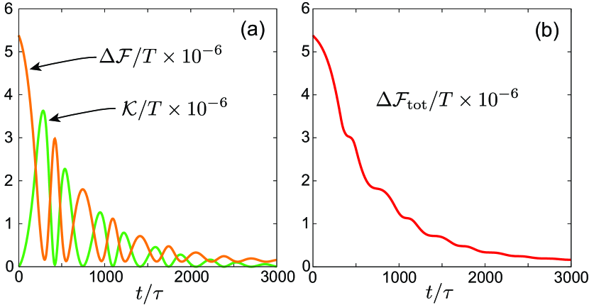
Figure 11: (a) DFT free energy deviation $\Delta{\cal F}(t)={\cal F}(t)-{\cal F}(\infty)$ and kinetic energy ${\cal K}(t)$ vs $t/\tau$. (b) Their sum ${\cal F}_{\rm tot}(t)$. Here, $\Delta{\cal F}(t)$ and ${\cal K}(t)$ exhibit a damped oscillation, but ${\cal F}_{\rm tot}(t)$ decreases monotonically in time.

IV.2.3 Damped oscillation

In Fig.10, we examine early-stage time-evolution in the range $0<t<5000\tau=560$ ps. The bubble radius undergoes a damped oscillation and approaches the final value $98.52d_{1}$, while the particle transport through the interface was negligible. The period is about $650\tau$ and the damping rate is about $5.1\times 10^{-4}\tau^{-1}$. We display (a) the bubble radius $R(t)$, which is defined as the peak position of $n_{2}(r,t)$ in our nonequilibrium situation (see Fig.9). In (b), we plot the liquid pressure $p_{\ell}(t)$ (taken at $r=170d_{1}$) and the gas pressure $p_{g}(t)$ (taken at $r=2d_{1}$), where the former exhibits a large damped oscillation but the latter variation is much smaller. The Laplace relation does not hold during the bubble oscillation. In (c), we show the solute density $n_{2}^{g}(t)$ and the total solute number within the bubble defined by $N_{2}^{b}(t)=\int_{r<R}d{\mbox{\boldmath$r$}}n_{2}({\mbox{\boldmath$r$}},t),$ Here, $n_{2}^{g}(t)$ largely oscillates, but $N_{2}^{b}(t)$ weakly increases only by a few $\%$. This implies that the solute transport through the interface is small and $n_{2}^{g}(t)\sim R(t)^{-3}$ in this time region. In addition, in (d), we show the profiles of the radial velocity $v(r,t)$ at four characteristic times.

In Fig.11, the kinetic energy ${\cal K}(t)$ in Eq.(82) and the DFT free energy deviation $\Delta{\cal F}(t)={\cal F}(t)-{\cal F}_{\infty}$ undergo damped oscillations out of phase with each other, where ${\cal F}_{\infty}$ is the final value of ${\cal F}$. However, their sum $\Delta{\cal F}_{\rm tot}(t)={\cal K}(t)+\Delta{\cal F}(t)$ decreases monotonically in time in accord with Eq.(83). Indeed, the radius deviation $\delta R$ from the mean radius (slightly smaller than $R_{\infty}$) approximately obeys

$$M{\ddot{R}}=-k\delta R-\zeta{\dot{R}}.$$ (88)

where ${\dot{R}}={d\delta R}/{dt}$ and ${\ddot{R}}={d^{2}\delta R}/{dt^{2}}$. We estimate $\zeta$ from $d\Delta{\cal F}/dt=-\zeta{\dot{R}}^{2}$, $k/M$ from the oscillation period, and $M$ from $M=2{\cal K}/{\dot{R}}^{2}$. Then, $M=3.9\rho R_{\infty}^{3}$, $k=2.1L/K_{\ell}$, and $\zeta=51\eta_{0}R_{\infty}$. Here, $\Delta{\cal F}$ arises from the change in the liquid volume, while it is given by the surface free energy ($\sim 4\pi\sigma R^{2}$) for $L\gg R$ Plesset ; Nepp ; Szeri ; sonol .

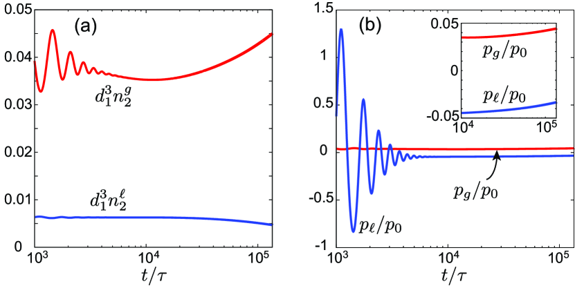
Figure 12: Long-time evolution ($t<1.3\times 10^{5}\tau$). (a) $d_{1}^{3}n_{2}^{g}(t)$ and $d_{1}^{3}n_{2}^{\ell}(t)$ vs $t/\tau$. For $t\gtrsim 10^{4}\tau$, $n_{2}^{g}(t)$ increases and $n_{2}^{\ell}(t)$ decreases slowly due to a solute flux into the bubble. (b) $p_{\ell}(t)/p_{0}$ and $p_{g}(t)/p_{0}$. Laplace law holds after the damped oscillation. They increase very slowly for $t\gtrsim 10^{4}\tau$ (inset) due to a small increase in $R(t)$.

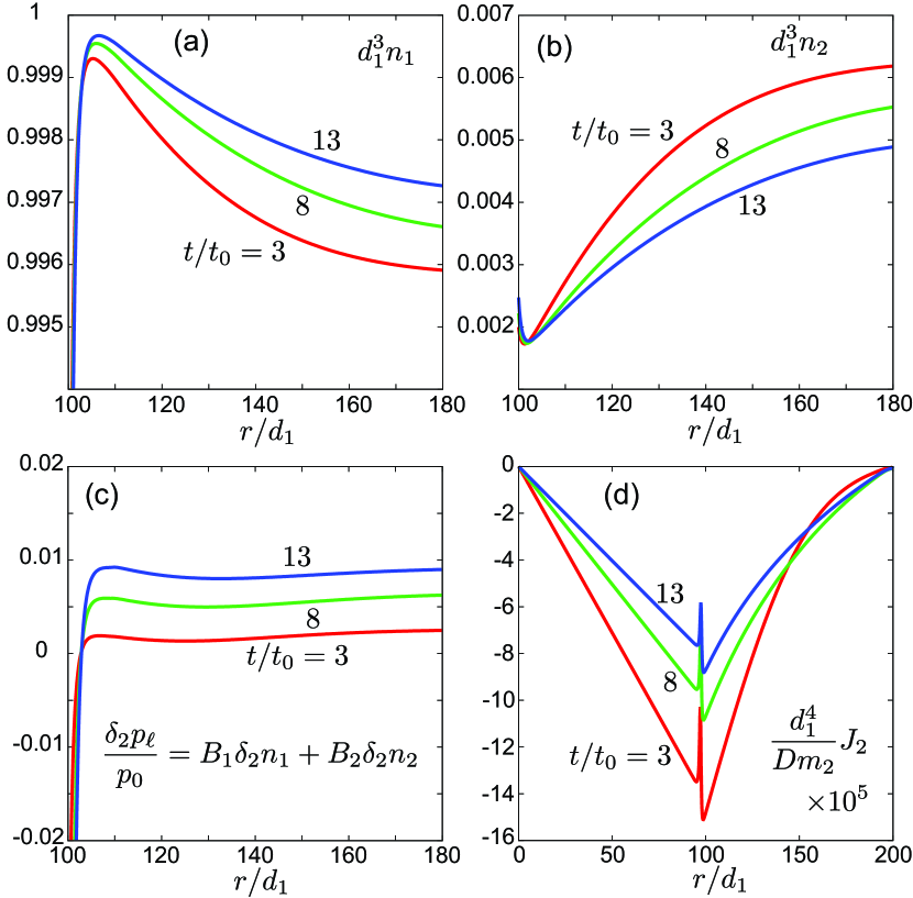
Figure 13: Profiles at $t/t_{0}=3$, 8, and 13 with $t_{0}=10^{4}\tau$. (a) $d_{1}^{3}n_{1}(r,t)$ and (b) $d_{1}^{3}n_{2}(r,t)$ in liquid. (c) Linear combination $\delta_{2}p_{\ell}/p_{0}\equiv B_{1}\delta_{2}n_{1}+B_{2}\delta_{2}n_{2}$, where $\delta_{2}n_{i}=n_{i}(r,t+t_{0})-n_{i}(r,t_{0})$ with $B_{1}=40.0d_{1}^{3}$ and $B_{1}=36.7d_{1}^{3}$. Here, $\delta_{2}p_{\ell}$ is equal to the pressure change $p(r,t+t_{0})-p(r,t_{0})$ from Eq.(40) and is homogeneous away from the interface. (b) Solute flux $J_{2}=\rho_{2}v+I(r,t)$ multiplied by $10^{5}d_{1}^{4}/Dm_{2}$.

IV.2.4 Long-time behavior

For $t>5000\tau$, the bubble radius $R(t)$ is close to the final one $R_{\infty}$, but small $n_{2}(r,t)$ still evolves diffusively in the liquid region. The final state should be reached on a timescale of $10^{7}\tau$. In our case, $K_{\ell}\cong 0.025/Tn_{1}^{\ell}$ and $L\cong 2R$, so that the compression pressure $\phi/K_{\ell}\sim 5p_{0}$ is much larger than the Laplace one $2\sigma/R\sim 0.1p_{0}$, where $p_{0}=Td_{1}^{-3}$. Moreover, from Eq.(40), the small pressure deviation remaining in bulk liquid is written as

$$\frac{p-p_{\infty}}{p_{0}}=B_{1}[n_{1}(r,t)-n_{1\infty}]+B_{2}[n_{2}(r,t)-n_{2\infty}],$$ (89)

where $p_{\infty}$, $n_{1\infty}$, and $n_{2\infty}$ are the final homogeneous values of $p$, $n_{1}$, and $n_{2}$ in liquid, respectively, $B_{1}=1/TK_{\ell}=40.0d_{1}^{3}$, and $B_{2}=d_{1}^{3}[1+n_{1}\nu_{s}^{\prime}(n_{1})]=36.7d_{1}^{3}$. Since $p$ should be homogeneous in liquid without sounds, this relation indicates that weak inhomogeneity of $n_{1}$ should be induced by that of $n_{2}$ in liquid.

In Fig.12, we plot $n_{2}^{g}(t)$ at $r=2d_{1}$ and $n_{2}^{\ell}(t)$ at $r=170d_{1}$ for $t<2\times 10^{5}\tau$. In (a), we can see a slow increase in $n_{2}^{g}(t)$ and a slow decrease in $n_{2}^{\ell}(t)$ for $t\gtrsim 10^{4}\tau$, due to the solute transport into the bubble. In (b), $p_{\ell}(t)$ and $p_{g}(t)$ satisfy the Laplace law after the damped oscillation. For $t\gtrsim 10^{4}\tau$, they increase slowly with the fixed difference, because of a small increase in $R$. Here, $R$ increases by $0.3d_{1}$ in time interval $[3t_{0},13t_{0}]$, producing a compressional pressure increase about $0.0135p_{0}$.

In Fig.13, we display profiles at $t/t_{0}=3$, 8, and 13 with $t_{0}=10^{4}\tau$. In (a), $n_{1}(r,t)$ exhibits inhomogeneity in accord with Eq.(89). Its overall increase is induced by the above-mentioned small increase in $R$. In (b), $n_{2}(r,t)$ relaxes diffusively far from the interface. In (c), we examine the incremental changes $\delta_{2}p_{\ell}\equiv p(r,t+t_{0})-p(r,t_{0})$ and $\delta_{2}n_{i}\equiv n_{i}(r,t+t_{0})-n_{i}(r,t_{0})$ in time interval $[t_{0},t_{0}+t]$. Then, the linear combination $\delta_{2}p_{\ell}/p_{0}\equiv B_{1}\delta_{2}n_{1}+B_{2}\delta_{2}n_{2}$ is surely homogeneous far from the interface.

In Fig.13(d), we display the solute flux $J_{2}(r,t)=\rho_{2}v+I$ in the radial direction (see Eq.(86)). Here, $v$ is nonvanishing only in the bubble interior, where $\rho_{2}=m_{2}n_{2}$ is uniform so that the gas is dilated by

$$v(r,t)=({\dot{R}}/{R})r.$$ (90)

At the interface $r=R$ (defined as the peak position of $n_{2}(r,t)$), $J_{2}(r,t)$ is slightly discontinuous across the peak of $n_{2}(r,t)$. This discontinuity gives rise to a change in the surface adsorption $\Gamma(t)$ in Eq.(57) as

$$\frac{d}{dt}\Gamma(t)=\frac{1}{m_{2}}[J_{2}(R-0,t)-J_{2}(R+0,t)].$$ (91)

In (d), the right hand side is of order $10^{-5}D/d_{1}^{4}=2.5\times 10^{-7}/d_{1}^{2}\tau$. In accord with this, $d_{1}^{2}\Gamma$ is 0.169, 0.185, and 0.211 at $t/t_{0}=3$, $8$, and 13, respectively, which indeed leads to $d\Gamma/dt\cong 3\times 10^{-7}/d_{1}^{2}\tau$.

V Summary and remarks

We have investigated statics and dynamics of phase separated states induced by a neutral low-density solute using DFT. At fixed $T=300$ K, we have assumed a considerably large solvation chemical potential $T\nu_{s}$ in liquid and a relatively weak solute-solute attractive interaction, under which small bubbles can appear in equilibriumnano ; review1 ; review2 . Main results in this paper are as follows.
(i) In Sec.II, we have presented some general relations in DFT for the stress tensor $\Pi_{\alpha\beta}$ in Eqs.(12), (15), and (19) and for the surface tension in Eqs.(21) and (25). The interface profiles of the densities $n_{i}(z)$ and the stress difference $\Delta\Pi(z)=\Pi_{zz}-\Pi_{xx}$ have been calculated in Fig.1. These quantities have algebraic tails away from the interface ($\propto|z-z_{\rm int}|^{-3}$ for Lennard-Jones potentials as in Fig.2). In particular, we have shown that the derivative $d\Delta\Pi/dz$ can be expressed in simple forms in DFT and in the exact statistical theory (Appendix B).
(iii) In Sec.III, we have calculated the solvation chemical potential $\mu_{s}=T\nu_{s}$ using the binary Carnahan-Starling modelCar in the dilute limit, as plotted in Fig.3. We have then calculated solute-induced deviations, such as the shift of the coexisting pressure $\Delta p_{\rm cx}$, in gas-liquid coexistence for dilute binary mixtures. We have also found small solute-rich bubbles, which are stable because they minimize the free energy functional of DFT. We have calculated the interface profiles of the densities and $\Delta\Pi$ for such bubbles in Fig.6.
(iv) In Sec.IV, we have investigated bubble dynamics using dynamic equations where DFT and the hydrodynamics are combined. We have described a damped oscillation with acoustic disturbances and a subsequent solute diffusion after a sudden decompression. In the late stage, weak solvent inhomogeneity is also induced such that the liquid pressure becomes homogeneous as in Fig.13.

We make some remarks. (1) We should calculate the profiles of surface bubbles on a wall in various conditions. The dewetting transition should be sensitive to a small amount of a solute (hydrophobic one for water)review2 . Bridging of two closely separated walls or colloidal particles by bubbles is also of great importance review1 ; review2 ; Yabu . (2) In our analysis, the solute is mildly adsorbed at the interface due to a minimum of $\nu_{s}(n_{1})$ in Eq.(38). More dramatic effects of adsorption should emerge with addition of surfactants and$/$or ions in the bubble formation. They are usually present in real water. (3) Bubble collapse after a pressure increase is also worth studying. In bubble dynamics, we will include inhomogeneous $T$ due to adiabatic density changes and latent heat in the scheme of the dynamic van der Waals theory Teshi ; Teshi1 ; Teshi2 ; vanderOnuki .

$$\eta_{i}=v_{0i}n_{i},\quad v_{0i}=\pi d_{i}^{3}/6\quad(i=1,2).$$ (A1)

The repulsive part of the free energy density $f_{h}$ in Eq.(1) is written as a function of the total volume fraction $\eta=\eta_{1}+\eta_{2}$. We here rewrite it in terms of $u=\eta/(1-\eta)$ as

$$\frac{f_{h}}{nT}=4u+u^{2}-\frac{3}{2}u[2y_{1}+(y_{1}+y_{2})u]+(y_{3}-1)g(u).$$ (A2)

The parameters $y_{1}$, $y_{2}$, and $y_{3}$ depend on $n_{1}$ and $n_{2}$ as

$$y_{1}=(1+\alpha)(1-\alpha)^{2}n_{1}n_{2}/n(n_{1}+\alpha^{3}n_{2}),$$ (A3)

$$y_{2}/y_{1}=\alpha(n_{1}+\alpha^{2}n_{2})/(1+\alpha)(n_{1}+\alpha^{3}n_{2}),$$ (A4)

$$y_{3}=[n_{1}+\alpha^{2}n_{2}]^{3}/n(n_{1}+\alpha^{3}n_{2})^{2},$$ (A5)

where $n=n_{1}+n_{2}$. In the one-component limit ($n_{2}\to 0)$Car0 , we have $y_{1}=y_{2}=y_{3}-1=0$. The function $g(u)$ in the last term in Eq.(A2) depends on $u$ as

$$g(u)=u-{u^{2}}/{2}-\ln(1+u).$$ (A6)

The pressure $p_{h}$ from $f_{h}$ in Eq.(9) is written as

$$\frac{p_{h}}{Tn}=(u+u^{2})[4+2u-3y_{1}-3(y_{1}+y_{2})u]+(1-y_{3})u^{3}$$

$$\hskip 5.69054pt=\frac{1+\eta+\eta^{2}}{(1-\eta)^{3}}-\frac{3(y_{1}+y_{2}\eta)\eta+y_{3}\eta^{3}}{(1-\eta)^{3}}-1.$$ (A7)

The chemical potential contributions $\mu_{hi}=\partial f_{h}/\partial n_{i}$ from $f_{h}$ in Eq.(6) are written as

$$\mu_{h1}=f_{h}/n-X_{1}+v_{01}p_{h}/\eta,$$ (A8)

$$\mu_{h2}=f_{h}/n+n_{1}X_{1}/n_{2}+v_{02}p_{h}/\eta,$$ (A9)

where $v_{0i}=\pi d_{ii}^{3}/6$. In terms of the derivatives $Y_{i}=\partial y_{i}/\partial n_{1}$ at fixed $n_{2}$, $X_{1}$ is written as

$$X_{1}=Tn[3u[Y_{1}+(Y_{1}+Y_{2})u]/2-Y_{3}g(u)].$$ (A10)

For small $n_{2}$ we have $y_{1}\cong(1+\alpha)(1+\alpha)^{2}n_{2}/n$, $y_{2}\cong\alpha(1+\alpha)^{2}n_{2}/n$, and $y_{3}-1\cong(3\alpha^{2}-2\alpha^{3}-1)n_{2}/n$ to linear order in $n_{2}$. From Eq.(A2), $f_{h}$ is then expanded as

$$f_{h}(n_{1},n_{2})=Tn_{1}({4u_{1}+u_{1}^{2}})+Tn_{2}\nu_{h}(n_{1})+\cdots,$$ (A11)

where $u_{1}=\eta_{1}/(1-\eta_{1})$ and $\nu_{h}$ is given in Eq.(33).

Appendix B: Statistical-mechanical theory of surface tension and interfacial stress

We consider binary particle systems with pairwise interactions, where the potential $\varphi_{ij}(r)$ includes attractive and repulsive parts. A planar interface is placed perpendicularly to the $z$ axis away from the walls at $z=0$ and $L$. Then, the average stress tensor can be expressed exactly as Irving ; Scho ; Kirk ; Onukibook

$$\Pi_{\alpha\beta}({\mbox{\boldmath$r$}})=Tn\delta_{\alpha\beta}-\int d{\mbox{\boldmath$r$}}_{1}\int d{\mbox{\boldmath$r$}}_{2}\sum_{ij}\frac{x_{12\alpha}x_{12\beta}}{2r_{12}}$$

$$\times\varphi^{\prime}_{ij}(r_{12})\delta_{s}({\mbox{\boldmath$r$}},{\mbox{\boldmath$r$}}_{1},{\mbox{\boldmath$r$}}_{2})\rho_{2}({\mbox{\boldmath$r$}}_{1},{\mbox{\boldmath$r$}}_{2}),$$ (B1)

in terms of the $\delta_{s}$ function in Eq.(11). This expression is analogous to that of DFT in Eq.(10). We introduce the two-body distribution function,

$$\rho_{ij}({\mbox{\boldmath$r$}}_{1},{\mbox{\boldmath$r$}}_{2})={\large\langle}{\sum_{k\neq\ell}\delta({\mbox{\boldmath$r$}}_{1}-{\mbox{\boldmath$R$}}_{k}^{i})\delta({\mbox{\boldmath$r$}}_{2}-{\mbox{\boldmath$R$}}_{\ell}^{j})}{\large\rangle},$$ (B2)

where ${\mbox{\boldmath$R$}}_{k}^{i}$ is the position of particle $k$ of species $i$. In Eq.(B1), the kinetic part $Tn\delta_{\alpha\beta}$ arises from the Maxwell-Boltzman distribution, while the second term holds even in nonequilibrium. Around a planar interface, we may set $\rho_{ij}({\mbox{\boldmath$r$}}_{1},{\mbox{\boldmath$r$}}_{2})=\rho_{ij}(z_{1},z_{2},r_{12})$ in equilibrium.

The surface tension is given by the Bakker formula in Eq.(25). After integration with respect to $z$, $x_{1}$, and $y_{1}$, we may remove the $\delta_{s}$ function to obtain the Kirkwood-Buff formula Kirk ; Ono ; Evansreview ; Scho ,

$$\sigma=\int d{z}_{1}\int d{\mbox{\boldmath$r$}}_{2}\sum_{ij}\frac{r_{12}^{2}-3z_{12}^{2}}{4r_{12}}\varphi^{\prime}_{ij}(r_{12})\rho_{ij}({\mbox{\boldmath$r$}}_{1},{\mbox{\boldmath$r$}}_{2}).$$ (B3)

We also consider the stress difference $\Delta\Pi(z)=\Pi_{zz}-\Pi_{xx}$ itself. Starting with Eq.(B1) we find

$$\Delta\Pi(z)=\pi\int_{z}^{L}dz_{1}\int_{0}^{z}dz_{2}\int_{z_{12}}^{\infty}du\sum_{ij}(u^{2}/z_{12}-3z_{12})$$

$$\hskip 28.45274pt\times{\varphi_{ij}^{\prime}(u)}\rho_{ij}(z_{1},z_{2},u),$$ (B4)

where $z_{1}>z>z_{2}$ and $z_{12}=z_{1}-z_{2}$. Use has been made of Eq.(18) and the relation $\int dx_{2}dy_{2}\delta(u-r_{12})=2\pi u\theta(u-|z_{12}|)$ at fixed $u$ and $z_{12}$. The $\sigma$ in Eq.(B3) and the $z$ integral of Eq.(B4) coincide. Analogously to Eq.(28), the derivative $d\Delta\Pi/dz$ can be written in the double integral form,

$$\frac{d}{dz}\Delta\Pi(z)={\pi}\int_{0}^{\infty}d\xi\int_{\xi}^{\infty}du\sum_{ij}(u^{2}/\xi-3\xi)\varphi_{ij}^{\prime}(u)$$

$$\hskip 28.45274pt\times[\rho_{ij}(z+\xi,z,u)-\rho_{ij}(z-\xi,z,u)].$$ (B5)

Here, if $z-z_{\rm int}\gg d_{1}$ and $\xi-z+z_{\rm int}\gg d_{1}$, we can neglect the pair correlation at the two points and are allowed to replace $\rho_{ij}(z+\xi,z,u)-\rho_{ij}(z-\xi,z,u)$ by $(n_{i}^{\ell}-n_{i}^{g})n_{j}^{\ell}\theta(\xi-z)$. Then, we obtain the tail in Eq.(29) if $\varphi_{ij}(r)\propto r^{-6}$ at long distances. If we replace $\varphi^{\prime}_{ij}(r_{12})\rho_{ij}({\mbox{\boldmath$r$}}_{1},{\mbox{\boldmath$r$}}_{2})$ in Eqs.(B3)-(B5) by $\phi^{\prime}_{ij}(r_{12})n_{i}(z_{1})n_{j}(z_{2})$ and $Tn$ in Eq.(B1) by $Tn+p_{h}$, we obtain their counterparts in DFT.

Appendix C: Efficient method of calculating equilibrium states in DFT

As a method of minimizing the free energy $\cal F$, we seek a stationary solution of the relaxation equations $(i=1,2)$,

$$\frac{\partial}{\partial\tau}n_{i}({\mbox{\boldmath$r$}},\tau)=-\mu_{i}({\mbox{\boldmath$r$}},\tau)+\langle{\mu_{i}}\rangle_{\rm cell}(\tau),$$ (C1)

where $\mu_{i}$ is the chemical potential in Eq.(5) determined by $n_{1}({\mbox{\boldmath$r$}},\tau)$ and $\langle{\mu_{i}}\rangle_{\rm cell}=\int d{\mbox{\boldmath$r$}}\mu_{i}/V$ is its space average in the cell. For any initial $n_{i}({\mbox{\boldmath$r$}},0)$, $\mu_{i}({\mbox{\boldmath$r$}},\tau)$ tend to be homogeneous as $\tau\to\infty$. Then, we obtain an equilibrium state with $n_{i}({\mbox{\boldmath$r$}})=\lim_{\tau\to\infty}n_{i}({\mbox{\boldmath$r$}},\tau)$. We assume the one-dimensional geometry in Fig.1 and the spherically symmetric geometry in Fig.6. Note that there is no physical meaning in this relaxation dynamics.

References

- (1) C. N. Likos, Phys. Rep. 348, 267 (2001).
- (2) J. Dzubiella and J.-P. Hansen, J. Chem. Phys. 121, 5514 (2004).
- (3) P. Hopkins, A. J. Archer, and R. Evans, J. Chem. Phys. 131, 124704 (2009).
- (4) H.S. Ashbaugh and M. E. Paulaitis, J. Am. Chem. Soc. 123, 10721 (2001).
- (5) D. Chandler, Nature, 437, 640 (2005).
- (6) S. Rajamani, T.M. Truskett, and S. Garde, Proc. Natl. Acad. Sci. U.S.A. 102, 9475 (2005).
- (7) D.Beysens and D.Esteve, Phys. Rev. Lett. 54, 2123 (1985).
- (8) D. Beysens and T. Narayanan, J. Stat. Phys. 95, 997 (1999).
- (9) F. Schlesener, A. Hanke, and S. Dietrich, J. Stat. Phys. 110, 981 (2003).
- (10) R. Okamoto and A. Onuki, Phys. Rev. E 88, 022309 (2013).
- (11) H. Tanaka and T. Araki, Chem. Eng. Sci.61. 2108 (2006).
- (12) T. Araki and H. Tanaka, J. Phys.: Condens. Matter, 20, 072101 (2008).
- (13) A. Furukawa, A. Gambassi, S. Dietrich , and H. Tanaka, Phys. Rev. Lett. 111, 055701 (2013).
- (14) S. Yabunaka, R. Okamoto, and A. Onuki, Soft Matter 11, 5738 (2015).
- (15) R. Okamoto and A. Onuki, Eur. Phys. J. E 38, 72 (2015).
- (16) P. Attard, M. P. Moody, and J.W.G. Tyrrell, Physica A 314, 696 (2002).
- (17) J. R. T. Seddon, D. Lohse, W. A. Ducker, and V. S. J. Craig, Chem. Phys. Chem. 13, 2179 (2012).
- (18) A. Onuki, R. Okamoto, and T. Araki, Bull. Chem. Soc. Jpn. 84, 569 (2011).
- (19) A.F. Kostko, M.A. Anisimov, J.V. Sengers, Phys. Rev. E 70, 026118 (2004).
- (20) R. Okamoto and A. Onuki, Phys. Rev. E 82, 051501 (2010).
- (21) D. E. Sullivan, Phys. Rev. B 20, 3991 (1979).
- (22) R. Evans, Adv. Phys. 28, 143 (1979).
- (23) P. Tarazona and R. Evans, Mol. Phys. 48, 799 (1983).
- (24) J. F. Lutsko, Adv. Chem. Phys. 144, 1 (2010).
- (25) N. F. Carnahan and K. E. Starling, J. Chem. Phys. 51, 635 (1969).
- (26) G. A. Mansoori, N. F. Carnahan, K. E. Starling, and T. W. Leland, J. Chem. Phys. 54, 1523 (1971).
- (27) J. W. Gibbs, Collected Works (Yale University Press, New Haven, CT, 1957), Vol. 1, pp. 219-331.
- (28) M. Blander and J. Katz, AIChE J. 21, 833 (1975).
- (29) M. E. M. Azouzi, C. Ramboz, J.-F. Lenain, and F. Caupin, Nat. Phys. 9, 38 (2013).
- (30) J. S. Langer and A, J. Schwrtz, Phys. Rev. A 21, 948 (1980).
- (31) A. Onuki, Phase Transition Dynamics (Cambridge University Press, Cambridge, 2002).
- (32) U. M. B. Marconi and P. Tarazona, J. Chem. Phys. 110, 8032 (1999).
- (33) A. J. Archer and R. Evans, J. Chem. Phys. 121, 4246 (2004).
- (34) M. Rex and H. Lwen, Eur. Phys. J. E 28, 139 (2009).
- (35) B. D. Goddard, A. Nold, N. Savva, G. A. Pavliotis, and S. Kalliadasis, Phys. Rev. Lett. 109, 120603 (2012).
- (36) A. Donev and E. Vanden-Eijnden, J. Chem. Phys.140, 234115 (2014).
- (37) A. Onuki, Phys. Rev. E 75, 036304 (2007).
- (38) J. D. van der Waals, Verh.-K. Ned. Akad. Wet., Afd. Natuurkd., Eerste Reeks 1(8), 56 (1893); English translation in : J. S. Rowlinson, J. Stat. Phys. 20, 197 (1979).
- (39) R. Teshigawara and A. Onuki, Europhys. Lett. 84, 36003 (2008).
- (40) R. Teshigawara and A. Onuki, Phys. Rev. E 82, 021603 (2010).
- (41) R. Teshigawara and A. Onuki, Phys. Rev. E 84, 041602 (2011).
- (42) M. S. Plesset and and A. Prosperetti, Ann. Rev. Fluid Mech. 9, 145 (1977).
- (43) M. M. Fyrillas and A. J. Szeri, J. Fluid Mech. 277, 381 (1994).
- (44) E. A. Neppiras, Phys. Rep. 61, 159 (1980).
- (45) M. P. Brenner, S. Hilgenfeldt, and D. Lohse, Rev. Mod. Phys. 74, 426 (2002).
- (46) J. W. Cahn, J. Chem. Phys. 66, 3667 (1977).
- (47) J. H. Irving and J. G. Kirkwood, J. Chem. Phys. 18, 817 (1949).
- (48) J.G. Kirkwood and F. P. Buff, J. Chem. Phys. 17, 338 (1949).
- (49) P. Schofield, J. R. Henderson Proc. R. Soc. Lond. A 379, 231 (1982).
- (50) F. P. Buff, R. A. Lovett, and F. H. Stillinger, Phys. Rev. Lett. 15, 621 (1965).
- (51) A. E. Ismail, G. S. Grest, and M. J. Stevens, J. Chem. Phys. 125, 014702 (2006).
- (52) G. Bakker, in: WIEN-HARMS’ Handbuch der Experimentalphysik VI. Leipzig: Akademische Verlagsgesellschaft 1928.
- (53) S. Ono and S. Kondo, Molecular Theory of Surface Tension in Liquids (Springer, Berlin, 1960).
- (54) J. A. Barker and J. R. Henderson J. Chem. Phys. 76, 6303 (1982).
- (55) J.A. Stbveng, T. Aukrust, and E.H. Hauge, Physica A 143, 40 (1987).
- (56) A. Onuki, J. Chem. Phys. 130, 124703 (2009).
- (57) A. Ben-Naim and Y. Marcus, J. Chem. Phys.81, 2016 (1984).
- (58) B. Guillot B. and Y. Guissani, J. Chem. Phys. 99, 8075 (1993).
- (59) G. Hummer, S. Garde, A. E. Garcia, and L. R. Pratt, Chem. Phys. 258, 349 (2000).
- (60) M. Ishizaki, H. Tanaka, and K. Koga, Phys. Chem. Chem. Phys. 13, 2328 (2011).
- (61) S. Zhao,R. Ramirez, R. Vuilleumier, and D. Borgis, J. Chem. Phys. 134, 194102 (2011).
- (62) R. Sander, Atmos. Chem. Phys. Discuss. 14, 29615 (2014).
- (63) F. L. Smith and A. H. Harvey, Chemical Engineering Progress, AIChE, 103, 33 (2007).
- (64) A. Onuki, EPL 82, 58002 (2008).
- (65) K. Binder, Physica A 319, 99 (2003).
- (66) V. Talanquer, C. Cunningham, and D. W. Oxtoby, J. Chem. Phys. 114, 6759 (2001).
- (67) T. Yamamoto and S. Ohnishi, Phys. Chem. Chem. Phys. 13, 16142 (2011).
- (68) L.D. Landau and E.M. Lifshitz, Fluid Mechanics (Pergamon, 1959).
- (69) J. O. Hirschfelder, C. F. Curtiss, and R. B. Bird, Molecular Theory of Gases and Liquids (Wiley, NewYork, 1954).
- (70) G.A. Fernandez, J. Vrabec, and H. Hasse, Fluid Phase Equilibria 221 (2004) 157 (2004).
- (71) K. Meier, A. Laesecke, and S. Kabelac, J. Chem. Phys. 121, 3671 (2004).
- (72) K. Meier, A. Laesecke, and S. Kabelac, J. Chem. Phys. 122, 014513 (2005).