Phase Transitions of Traveling Salesperson Problems solved with Linear Programming and Cutting Planes

Abstract

The Traveling Salesperson problem asks for the shortest cyclic tour visiting a set of cities given their pairwise distances and belongs to the NP-hard complexity class, which means that with all known algorithms in the worst case instances are not solveable in polynomial time, i.e., the problem is hard. Though that does not mean, that there are not subsets of the problem which are easy to solve. To examine numerically transitions from an easy to a hard phase, a random ensemble of cities in the Euclidean plane given a parameter $\sigma$, which governs the hardness, is introduced. Here, a linear programming approach together with suitable cutting planes is applied. Such algorithms operate outside the space of feasible solutions and are often used in practical application but rarely studied in physics so far. We observe several transitions. To characterize these transitions, scaling assumptions from continuous phase transitions are applied.

The Traveling Salesperson Problem (TSP) Cook (2012) is to find the shortest tour through a given set of cities, with known pairwise distances, and going back to the initial city. TSP belongs to the class of NP-hard optimization problems Arora and Barak (2009), where so far only algorithms with exponentially growing worst-case running time are known. Thus, a good tour optimization can not only save money when used for real world applications, but also it has a history as a testbed for exact Applegate et al. (2003); Cook (2012) as well as heuristic optimization algorithms, e.g., simulated annealing Kirkpatrick et al. (1983), taboo search Glover (1986) or ant colony algorithms Dorigo and Gambardella (1997). Also, for the TSP there exist specific heuristics Lin and Kernighan (1973); Dorigo and Gambardella (1997); Hougardy and Schroeder (2014). For the Euclidean case (which is still NP-hard Papadimitriou (1977)), i.e., the pairwise distances are the Euclidean distances, a polynomial-time approximation scheme Arora (1998) is known. For special corner cases Burkard et al. (1995) even polynomial-time algorithms exist.

Interestingly, NP-complete problems often show phase transitions Hartmann and Weigt (2006); Mezard and Montanari (2009); Mertens (2006) where instances are typically easy to solve in one region and typically hard in the other region. Some of the classical NP-complete problems Karp (1972) were examined with respect to phase transitions with methods of statistical mechanics in Ref. Martin et al. (2001); Biroli et al. (2002); Weigt and Hartmann (2000); Hartmann and Weigt (2003); Krzakała et al. (2007). Note that in the statistical mechanics literature usually algorithms like branch-and-bound Papadimitriou and Steiglitz (1998); Weigt and Hartmann (2001); Cocco and Monasson (2001), stochastic search Schneider and Kirkpatrick (2006) and message-passing algorithms Mézard et al. (2002) are studied which operate inside the space of feasible configurations. In contrast, for practical applications, algorithms based on linear programming (LP) dominate because they are very efficient. These LP-based algorithms operate outside the space of feasible solutions and they should be given more attention in the physics community. For this reasons we study here LP algorithms with respect to phase transitions for the TSP.

In Ref. Gent and Walsh (1996) the Euclidean TSP decision problem on random realizations of cities scattered on the unit square was under scrutiny and shows a “transition” when asking when the tour length exceeds a certain rescaled threshold. But here the two “phases” are not with respect to basic properties of the instances, there is no parametrized ensemble. Rather, the instances are sorted into two classes after they are solved, basically reflecting the typical growth of the tour length. Instead, here we define a parametrized ensemble of TSP instances. We study the solvability by a polyonmial-time standard LP approach together with several types of so-called cutting-planes. We find several “easy–hard” transitions, similar to one previously found for the vertex-cover problem Dewenter and Hartmann (2012); Takabe and Hukushima (2013).

The two-dimensional Euclidean TSP is under scrutiny Percus and Martin (1996); Gent and Walsh (1996). Each city from the set of cities $V$ has coordinates on a plane determining the pairwise distances $c_{ij}$ as their Euclidean distances, in particular  $c_{ij}=c_{ji}$. We generated each instance of $N$ cities by random displacement of cities from a well defined start configuration, chosen as $N$ cities lying on a circle with a circumference of $2\pi N$, i.e., the distance between two neighboring cities is approximately $1$. Note that for the circle even the most simple greedy heuristics, e.g., nearest neighbor, finds the optimal tour. Further the circle fulfills the necklace condition Edelsbrunner et al. (1989) which enables a polynomial-time solution algorithm and all points are part of the convex hull which also solves the tour Flood (1956). For each city the displacement is determined by two independent random variables from an uniform distribution. $\phi\in[0,2\pi)$ is treated as a displacement angle and $r\in[0,\sigma]$ as a radius, such that the new position of a city lies inside of a disk with radius $\sigma$ around its initial position. Four sample instances together with their optimal tours for $N=1024$ cities are shown in Fig. 1.

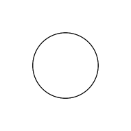
(a) $\sigma=0$

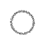
(b) $\sigma=20$

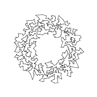
(c) $\sigma=80$

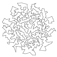
(d) $\sigma=160$

Figure 1: Evolution of a $N=1024$ and $R=\frac{N}{2\pi}\approx 160$ system with increasing disorder $\sigma$. These sample realizations were solved with Concorde Applegate et al. (2003). Obviously the leftmost configuration is easy to solve, but the other three are probably not.

Next, we present our numerical approach. LPs can be solved in polynomial-time using the ellipsoid algorithm Papadimitriou and Steiglitz (1998). In this study the simplex algorithm Papadimitriou and Steiglitz (1998) implemented by the commercial optimization library CPLEX is used instead, for its good runtime behavior in the typical case. If there are constraints which enforce the variables to be integer, it is called integer program (IP) which also belongs to the class of NP-hard problems. One can formulate the TSP as an integer program with the objective Eq. (1) and the constraints Eq. (2) to (4) Dantzig et al. (1954).

minimize $$\sum_{i}\sum_{j<i}c_{ij}x_{ij}$$ (1)

subject to $$x_{ij} \in\{0,1\}$$ (2)

$$\sum_{j}x_{ij} =2 \forall i\in V$$ (3)

$$\sum_{i\in S,j\notin S}x_{ij} \geq 2 \forall S\varsubsetneq V,S\neq\varnothing$$ (4)

Where the variables $x_{ij}$ are $1$ if $i$ and $j$ are consecutive in the tour, and $0$ otherwise. The objective Eq. (1) minimizes the tour length. The integer constraints Eq. (2) restrict $x_{ij}$ to the integers $0$ and $1$, the degree constraints Eq. (3) ensure that every city has exactly two neighbors, one for the salesperson to enter one to leave. And the subtour elimination constraints (SEC) Eq. (4) prevent closed subtours, i.e., loops which visit just a subset of all cities, by forcing at least two edges to cross the boundaries of all sets $S\varsubsetneq V,S\neq\varnothing$, which ensures that the salesperson can enter and leave the set. Hence a closed subtour would violate the constraint for the set $S$ which contains all cities of the subtour. Note that there are exponentially many SECs, because there are exponentially many different subsets $S\subset V$. To solve this integer program, it is first relaxed to a LP, i.e., Eq. (2) is replaced by $x_{ij}\in[0,1]$. The solution of this LP relaxation will always have a better or equal tour length than the solution of the TSP, but may not always be a valid tour, i.e., may have fractional $x_{ij}$. Though, if the solution of a LP relaxation is integer, it is guaranteed to be the optimal tour.

Because there are exponentially many SECs, they will not be enforced in the beginning, instead SECs will be added if violated by the current LP solution, and the resulting LP is solved again. The violated SECs can be found by a global minimum cut, e.g., with the Stör-Wagner algorithm in polynomial-time Stör and Wagner (1997). This is iterated until no violated SEC exists anymore.

A measure of hardness of an instance for a given LP algorithm is as follows: if the LP relaxation results in all variables being integer, i.e., if the instance can be solved in polynomial time Grötschel et al. (1981, 1993); Conforti et al. (2014), it is therefore easy. Also we will look at the degree LP relaxation where the SECs are removed and only the degree constraints (3) and the bounds are enforced. Here, we also find instances which are solved by this simpler algorithm. Thus, they can be considered even easier.

Note that this algorithm can easily be extended to find always the optimal solution, by a branch-and-cut search Applegate et al. (2003) at the cost of a worst-case exponential running time. Nevertheless, here we are mostly interested in the algorithm-dependent hardness of an instance, not necessarily in always finding a solution. The focus on the solvability by LP methods allows reasonable big instances of up to $N=1448$ cities at $80$ different $\sigma\in[0,60]$ and $5000$ samples each. All errorbars are obtained via bootstrap resampling Efron (1979); Hartmann (2015); Young (2015) if not noted otherwise.

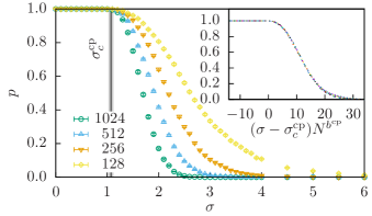
Figure 2: (color online) Probability $p$ that the LP relaxation is integer, i.e., the solution can be obtained by LP, as a function of the displacement parameter $\sigma$. The inset shows the same $p$ for $N\geq 256$ plotted with a rescaled $\sigma$-axis with $\sigma_{c}^{\mathrm{cp}}=1.07(5)$ and ${b^{\mathrm{cp}}}=0.43(3)$ obtained by Fig. 3. Different symbols and errorbars are omitted for clarity.

The probability $p$ to find the true integer solution using the LP relaxation is plotted in Fig. 2. For small disorder, $p$ is constant at $p=1$ and falls with increasing $\sigma$ to $p=0$. With increasing system size $N$ the curves become steeper. This pattern is typical for a phase transition. Therefore, the results indicate a phase transition from an easy phase, where the instances are typically solvable by polynomial-time linear programming techniques, to a hard phase.

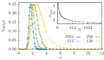
Figure 3: (color online) Variance of the solution probability $\operatorname{Var}(p)$ as a function of the disorder $\sigma$. The inset shows the position of maximal variance of the solution probability $p$ over the number of cities $N$. The positions are obtained by second order polynomials fitted to the 5 data points next to the peak. The power-law $\sigma=aN^{-{b^{\mathrm{cp}}}}+\sigma_{c}^{\mathrm{cp}}$ is fitted to the peak positions for $N\geq 256$ to minimize the effects of corrections to scaling, yielding $\sigma_{c}^{\mathrm{cp}}=1.07(5)$ and ${b^{\mathrm{cp}}}=0.43(3)$.

Next, we determined the transition point $\sigma_{c}^{\mathrm{cp}}$ in the limit $N\to\infty$ and the exponent ${b^{\mathrm{cp}}}$, governing the finite-size scaling behavior Goldenfeld (1992) near the transition point, corresponding to the correlation-length exponent for physical systems. For this purpose we fitted parabolas to the variance of $p$ in vincinity of the maximum, see Fig. 3. For second-order phase transitions the peak positions are expected to follow $\sigma=\sigma_{c}^{\mathrm{cp}}+aN^{-{b^{\mathrm{cp}}}}$, which holds well for our data as depicted in the inset of Fig. 3.

According to finite-size scaling, rescaling the $\sigma$ axis according to $(\sigma-\sigma_{c}^{\mathrm{cp}})N^{{b^{\mathrm{cp}}}}$ should yield a collapse of the data onto one curve Binder and Heermann (2010) for big values of $N$ in vicinity of the critical point. This is true for our data as visible in the inset of Fig. 2. confirming the values of $\sigma_{c}^{\mathrm{cp}}$ and ${b^{\mathrm{cp}}}$.

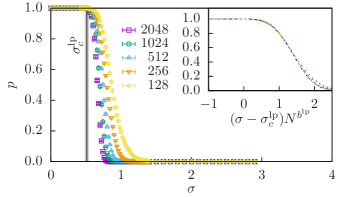
Figure 4: (color online) Probability $p$ that the degree LP relaxation is integer. The inset shows the collapse for $N\geq 256$, with $\sigma_{c}^{\mathrm{lp}}=0.51(4)$ and $b^{\mathrm{lp}}=0.29(6)$ obtained from the same type of analysis as in Fig. 3 for $N\geq 512$.

To identify a region of even easier instances, we studied also the LP with applying only the degree contraints (3), see Fig. 4. We found a second easy–hard transition with $\sigma_{c}^{\mathrm{lp}}=0.51(4)$ and $b^{\mathrm{lp}}=0.29(6)$.

A further class of cutting-plane inequalities for the TSP are blossom inequalities Padberg and Rao (1982) which originate from the two-matching LP Edmonds (1965). A subset, which is easy to separate using heuristics, are fast blossoms Applegate et al. (2003), available in Concorde Applegate et al. (2003). Doing the same analysis as above revealed a third transition (not shown) at $\sigma_{c}^{\mathrm{fb}}=1.47(8)$ with $b^{\mathrm{fb}}=0.40(3)$.

Next, we want to find out whether the easy–hard transitions are accompanied by changes of suitably defined structural order parameters. For up to $N=180$ the optimal tours for all studied samples were obtained by a branch-and-cut procedure, available in CPLEX, to examine structural properties of the solutions. With increasing value of $\sigma$ optimized tours appear to be more “meandering” as shown in Fig. 1. As a measure of this “meandering”, we used the tortuosity, as defined in Ref. Grisan et al. (2003), where it was used to evaluate images of blood vessels in the retina to detect vascular diseases. To calculate $\tau$, the tour is segmented into $n$ segments, such that each segment has the same curvature sign and is of maximal length. Let the arc length $L_{i}$ be the length of the segment $i$ along the tour and let the chord length $S_{i}$ be the direct distance between the first and last city of the segment $i$ and $L$ the total length of the tour. Then the tortuosity is defined as

$$\tau=\frac{n-1}{L}\sum_{i=1}^{n}\left(\frac{L_{i}}{S_{i}}-1\right).$$ (5)

Figure 5: (color online) The tortuosity $\tau$ of optimal tours as a function of the displacement parameter $\sigma$ for different system sizes $N\leq 180$ peaks at $\sigma_{c}^{\mathrm{\tau}}$, which coincides with $\sigma_{c}^{\mathrm{cp}}$ determined by the fit in Fig. 3 (gray bar $=$ mean $+$ error). On the right side the same is done with data from a slightly modified model, explained later in the text.

When plotting $\tau$ as a function of $\sigma$ in Fig. 5, it shows peaks near $\sigma_{c}^{\mathrm{cp}}$. As a very rough estimate of the position of this peak, straight lines are fitted to $\tau$ at $N=180$ left and right of the peak and their intersection is interpreted as an estimate of the peak positions, with errors obtained by error propagation. This is shown for $N=180$ in Fig. 5 and done for all sizes $N\geq 64$. Via a power-law fit to $\sigma^{\mathrm{\tau}}=\sigma_{c}^{\mathrm{\tau}}+aN^{-c}$, we estimated an asymptotic $\sigma_{c}^{\mathrm{\tau}}=1.06(23)$, which is consistent with the estimate $\sigma_{c}^{\mathrm{cp}}$ from Fig. 3, Unfortunately the fit is not good enough to give a meaningful estimate of the more susceptible corresponding exponent $b^{\mathrm{\tau}}$.

Comparing the solution tour $x_{ij}$ to the circular shaped optimal tour at $\sigma=0$, it is expected that they are similar at very small disorder $\sigma$. A way to measure this similarity is to look at the number of edges occurring in the one tour but not in the other, i.e., the Hamming distance Hamming (1950).

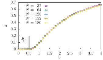
Figure 6: (color online) Difference of the optimal tour to the initial circle as a function of $\sigma$.

The tour difference $d$ shown in Fig. 6 is the Hamming distance normalized by $2N$, such that two tours with no common edges would result in $d=1$ while two tours visiting the cities in the same sequence would result in $d=0$. This observable seems to be roughly independent of $N$. Fig. 6 suggests that the easy–hard transition observed when using the degree LP relaxation alone corresponds to the structural change observed by studying the hamming distance $d$.

Unfortunately, we were not able to indentify so far an observable which corresponds to the phase transition occurring when using the fast blossoms.

We performed the same analysis for a different random ensemble, where the cities are displaced by $\Delta x$ and $\Delta y$ from a Gaussian distribution $G(0,\sigma)$ for each direction. As expected for continuous phase transitions, we obtained (not shown) the same critical exponent $b^{\mathrm{cp,g}}=0.45(5)$ within errorbars, which hints that this model exhibits universality with respect to the type of disorder. The resulting values are shown in Tab. 1. Also for the case of cities displaced spherical by $\phi$, $\theta$ and $r$ from uniform distributions in three dimensions it shows the same critical exponent $b^{\mathrm{cp,3}}=0.40(4)$. Note that unlike many other models (e.g. Ising ferromagnet or percolation) the different dimension does not lead to a different exponent.

	$\sigma_{c}$		$b$
with SEC	$\sigma_{c}^{\mathrm{cp}}=$	$1.07(5)$	${b^{\mathrm{cp}}}=$	$0.43(3)$
	$\sigma_{c}^{\mathrm{\tau}}=$	$1.06(23)$		–
	$\sigma_{c}^{\mathrm{cp,g}}=$	$0.47(3)$	$b^{\mathrm{cp,g}}=$	$0.45(5)$
	$\sigma_{c}^{\mathrm{\tau,g}}=$	$0.44(8)$		–
	$\sigma_{c}^{\mathrm{cp,3}}=$	$1.18(8)$	$b^{\mathrm{cp,3}}=$	$0.40(4)$
only degree	$\sigma_{c}^{\mathrm{lp}}=$	$0.51(4)$	$b^{\mathrm{lp}}=$	$0.29(6)$
fast blossoms	$\sigma_{c}^{\mathrm{fb}}=$	$1.47(8)$	$b^{\mathrm{fb}}=$	$0.40(3)$

Table 1: Values of critical points and exponents grouped by different types of transitions.

We have shown that for this random ensemble governed by the parameter $\sigma$ there exist various easy–hard phase transitions. This indicates a rich behavior of the ensemble with respect to the typical computational hardness. Furthermore, at least for two cases we found that the transitions can be correlated with measurable changes of the solution structure, namely Hamming distance to the circle solution and tortuosity, respectively. The transitions can be characterized by critical exponents $b$. Within the statistical accuracy of our data, the critical exponents for the different easy–hard transitions are compatible within two sigma.

An interesting question for further study would be finding an answer to why the tortuosity $\tau$ peaks at $\sigma_{c}$, where the TSP becomes not solvable using LP and SEC. Unfortunately $\tau$ is quite complex to measure. Therefore the search for a simpler observable showing the transition would be of equal interest.

Besides the blossom inequalities, there are more complicated inequalities valid for the TSP establishing facets on the polytope, which can be implemented as cutting planes and partly already be separated in polynomial-time Fleischer et al. (2006). It would be interesting if those would establish a further phase transition at higher $\sigma$ and if the critical exponent $b$ stays the same.

In general, LP-based algorithms are used a lot in practice and it would be of great interest to study suitable ensembles of other NP-hard optimization problems with respect to easy–hard transitions. Furthermore, a statistical-mechanics analysis of the performance of LP-based algorithms, like done in the past for branch-and-bound algorithms Weigt and Hartmann (2001); Cocco and Monasson (2001), would yield more insight into the sources of computational hardness.

References

- Cook (2012) W. Cook, In Pursuit of the Traveling Salesman: Mathematics at the Limits of Computation (Princeton University Press, 2012), ISBN 9780691152707, URL https://books.google.de/books?id=S3bxbr_-qhYC.
- Arora and Barak (2009) S. Arora and B. Barak, Computational complexity: a modern approach (Cambridge University Press, 2009).
- Applegate et al. (2003) D. Applegate, R. Bixby, V. Chvátal, and W. Cook, Mathematical programming 97, 91 (2003).
- Kirkpatrick et al. (1983) S. Kirkpatrick, M. Vecchi, et al., Science 220, 671 (1983).
- Glover (1986) F. Glover, Computers and Operations Research 13, 533 (1986), ISSN 0305-0548, applications of Integer Programming, URL http://www.sciencedirect.com/science/article/pii/0305054886900481.
- Dorigo and Gambardella (1997) M. Dorigo and L. M. Gambardella, Evolutionary Computation, IEEE Transactions on 1, 53 (1997), see papercore summary http://www.papercore.org/Dorigo1997.
- Lin and Kernighan (1973) S. Lin and B. W. Kernighan, Operations research 21, 498 (1973).
- Hougardy and Schroeder (2014) S. Hougardy and R. T. Schroeder, in Graph-Theoretic Concepts in Computer Science, edited by D. Kratsch and I. Todinca (Springer International Publishing, 2014), vol. 8747 of Lecture Notes in Computer Science, pp. 275–286, ISBN 978-3-319-12339-4, URL http://dx.doi.org/10.1007/978-3-319-12340-0_23.
- Papadimitriou (1977) C. H. Papadimitriou, Theoretical Computer Science 4, 237 (1977), ISSN 0304-3975, URL http://www.sciencedirect.com/science/article/pii/0304397577900123.
- Arora (1998) S. Arora, Journal of the ACM (JACM) 45, 753 (1998).
- Burkard et al. (1995) R. E. Burkard, V. G. Deineko, R. van Dal, J. A. A. van der Veen, and G. J. Woeginger, Well-solvable special cases of the tsp: A survey (1995), URL http://citeseerx.ist.psu.edu/viewdoc/summary?doi=10.1.1.48.1273.
- Hartmann and Weigt (2006) A. K. Hartmann and M. Weigt, Phase transitions in combinatorial optimization problems: basics, algorithms and statistical mechanics (John Wiley & Sons, 2006).
- Mezard and Montanari (2009) M. Mezard and A. Montanari, Information, physics, and computation (Oxford University Press, 2009).
- Mertens (2006) S. Mertens, The Nature of Computation (John Wiley & Sons, 2006).
- Karp (1972) R. M. Karp, Reducibility among combinatorial problems (Springer, 1972).
- Martin et al. (2001) O. C. Martin, R. Monasson, and R. Zecchina, Theoretical computer science 265, 3 (2001).
- Biroli et al. (2002) G. Biroli, S. Cocco, and R. Monasson, Physica A: Statistical Mechanics and its Applications 306, 381 (2002), ISSN 0378-4371, invited Papers from the 21th IUPAP International Conference on Statistical Physics, URL http://www.sciencedirect.com/science/article/pii/S0378437102005162.
- Weigt and Hartmann (2000) M. Weigt and A. K. Hartmann, Phys. Rev. Lett. 84, 6118 (2000), see papercore summary http://www.papercore.org/Weigt2000, URL http://link.aps.org/doi/10.1103/PhysRevLett.84.6118.
- Hartmann and Weigt (2003) A. K. Hartmann and M. Weigt, Journal of Physics A: Mathematical and General 36, 11069 (2003), URL http://stacks.iop.org/0305-4470/36/i=43/a=028.
- Krzakała et al. (2007) F. Krzakała, A. Montanari, F. Ricci-Tersenghi, G. Semerjian, and L. Zdeborová, Proceedings of the National Academy of Sciences 104, 10318 (2007), see papercore summary http://www.papercore.org/Krzakala2007.
- Papadimitriou and Steiglitz (1998) C. Papadimitriou and K. Steiglitz, Combinatorial Optimization: Algorithms and Complexity, Dover Books on Computer Science Series (Dover Publications, 1998), ISBN 9780486402581, URL http://books.google.de/books?id=u1RmDoJqkF4C.
- Weigt and Hartmann (2001) M. Weigt and A. K. Hartmann, Phys. Rev. Lett. 86, 1658 (2001).
- Cocco and Monasson (2001) S. Cocco and R. Monasson, Phys. Rev. Lett. 86, 1654 (2001).
- Schneider and Kirkpatrick (2006) J. J. Schneider and S. Kirkpatrick, Stochastic Optimization (Springer, Heidelberg, 2006).
- Mézard et al. (2002) M. Mézard, G. Parisi, and R. Zecchina, Science 297, 812 (2002).
- Gent and Walsh (1996) I. P. Gent and T. Walsh, Artificial Intelligence 88, 349 (1996), ISSN 0004-3702, URL http://www.sciencedirect.com/science/article/pii/S0004370296000306.
- Dewenter and Hartmann (2012) T. Dewenter and A. K. Hartmann, Physical Review E 86, 041128 (2012), see papercore summary http://www.papercore.org/Dewenter2012.
- Takabe and Hukushima (2013) S. Takabe and K. Hukushima, J. Phys. Soc. Jap. 83, 043801 (2013).
- Percus and Martin (1996) A. G. Percus and O. C. Martin, Physical Review Letters 76, 1188 (1996).
- Edelsbrunner et al. (1989) H. Edelsbrunner, G. Rote, and E. Welzl, Theoretical Computer Science 66, 157 (1989), ISSN 0304-3975, URL http://www.sciencedirect.com/science/article/pii/0304397589901333.
- Flood (1956) M. M. Flood, Operations Research 4, 61 (1956), eprint http://dx.doi.org/10.1287/opre.4.1.61, URL http://dx.doi.org/10.1287/opre.4.1.61.
- Dantzig et al. (1954) G. Dantzig, R. Fulkerson, and S. Johnson, Journal of the Operations Research Society of America 2, 393 (1954), see papercore summary http://www.papercore.org/Dantzig1954.
- Stör and Wagner (1997) M. Stör and F. Wagner, Journal of the ACM (JACM) 44, 585 (1997), see papercore summary http://www.papercore.org/Stoer1997.
- Grötschel et al. (1981) M. Grötschel, L. Lovász, and A. Schrijver, Combinatorica 1, 169 (1981).
- Grötschel et al. (1993) M. Grötschel, L. Lovász, and A. Schrijver, Algorithms and Combinatorics 2, 1 (1993).
- Conforti et al. (2014) M. Conforti, G. Cornuéjols, and G. Zambelli, in Integer Programming (Springer International Publishing, 2014), vol. 271 of Graduate Texts in Mathematics, pp. 281–319, ISBN 978-3-319-11007-3, URL http://dx.doi.org/10.1007/978-3-319-11008-0_7.
- Efron (1979) B. Efron, Ann. Statist. 7, 1 (1979), URL http://dx.doi.org/10.1214/aos/1176344552.
- Hartmann (2015) A. K. Hartmann, Big Practical Guide to Computer Simulations (World Scientific, 2015), URL http://www.worldscientific.com/doi/abs/10.1142/9789814571784_0008.
- Young (2015) A. P. Young, Everything You Wanted to Know About Data Analysis and Fitting but Were Afraid to Ask, SpringerBriefs in Physics (Springer International Publishing, 2015), ISBN 978-3-319-19050-1, URL http://dx.doi.org/10.1007/978-3-319-19051-8_2.
- Goldenfeld (1992) N. Goldenfeld, Lectures on phase transitions and the renormalization group (Addison-Wesely, Reading (MA), 1992).
- Binder and Heermann (2010) K. Binder and D. W. Heermann, Monte Carlo Simulation in Statistical Physics (Springer, Berlin Heidelberg, 2010), ISBN 978-3-642-03162-5.
- Padberg and Rao (1982) M. W. Padberg and M. R. Rao, Mathematics of Operations Research 7, 67 (1982).
- Edmonds (1965) J. Edmonds, J. Res. Nat. Bur. Standards B 69, 125 (1965).
- Grisan et al. (2003) E. Grisan, M. Foracchia, and A. Ruggeri, in Engineering in Medicine and Biology Society, 2003. Proceedings of the 25th Annual International Conference of the IEEE (2003), vol. 1, pp. 866–869 Vol.1, ISSN 1094-687X.
- Hamming (1950) R. W. Hamming, Bell System Technical Journal 29, 147 (1950).
- Fleischer et al. (2006) L. K. Fleischer, A. N. Letchford, and A. Lodi, Mathematics of Operations Research 31, 696 (2006).