Multiplexing Free-Space Channels using Twisted Light

Abstract

We experimentally demonstrate an interferometric protocol for multiplexing optical states of light, with potential to become a standard element in free-space communication schemes that utilize light endowed with orbital angular momentum (OAM). We demonstrate multiplexing for odd and even OAM superpositions generated using different sources. In addition, our technique permits one to prepare either coherent superpositions or statistical mixtures of OAM states. We employ state tomography to study the performance of this protocol, and we demonstrate fidelities greater than 0.98.

I Introduction

Beams of light that are structured in their transverse degree of freedom are an interesting and powerful tool in quantum information science due the virtually limitless level of complexity than can be encoded onto this structure. One such promising set of modes is the orbital angular momentum (OAM) states introduced by Allen et al. Allen et al. (1992). Such modes have a spiral phase profile $\exp(i\ell\phi)$, where $\phi$ is the azimuthal transverse angle, and $\ell$ is the unbounded mode index which specifies the amount of OAM per photon in units of $\hbar$. The usefulness of such modes has already been demonstrated in communication (both classical and quantum) Gibson et al. (2004); Wang et al. (2012); Tamburini et al. (2012); Mirhosseini et al. (2015), as well as a fundamental tool in basic quantum information science Mair et al. (2001); Molina-Terriza et al. (2007); Nagali et al. (2009).

It was recently demonstrated that OAM states, could be transformed to implement a “Quantum Hilbert Hotel” Potoček et al. (2015). For instance, for states with OAM index $\ell$, a setup could be built implementing a Hibert hotel map $\mathbb{H}_{2}$ that transforms $\mathbb{H}_{2}\ket{\ell}=\ket{2\ell}$. This means that even if one had a state that contained an infinite amount of information by utilizing the entire countably infinite OAM basis, more information could always be added by a transformation of the state, i.e. an arbitrary state can be written as $\ket{\psi}=\sum_{\ell}\psi_{\ell}\ket{\ell}$, in which case the Hilbert hotel map would transform this to

$$\mathbb{H}_{2}\ket{\psi}=\sum_{\ell}\psi_{\ell}\ket{2\ell},$$ (1)

leaving the amplitude in all the odd numbered OAM states identically zero. However, in order to utilize this transformation for quantum information processing, it is essential to be able to address both the even and odd OAM subspaces separately and then be able to coherently combine them.

In this paper we experimentally implement such an OAM multiplexer that allows for the coherent combination of the even and odd order OAM modes as proposed in Ref. García-Escartín and Chamorro-Posada (2008). This device interferometrically combines multiple beams in a manner that is in principle both reversible and completely lossless, as is necessary for many quantum applications Leach et al. (2002). As has been pointed out, such a multiplexer is also useful for classical multiplexing of information for use in communication as well Gatto et al. (2011); Martelli et al. (2011).

II OAM Multiplexer

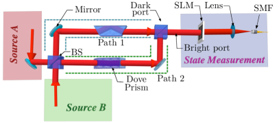
Figure 1: Basic schematic for OAM multiplexer. The device combines the symmetric part of input beam $A$ with the antisymmetric part of $B$.

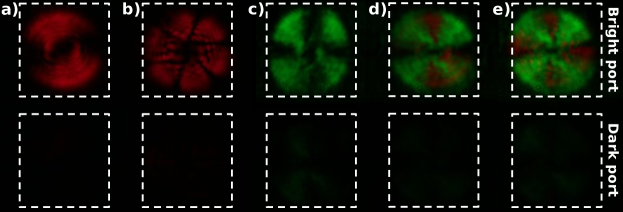
Figure 2: Experimental evidence of the functionality of the OAM duplexer. Part a) and b) show the two output ports when only source $A$ is active with the antisymmetric states $\ket{\psi_{1}}=1/\sqrt{2}(\ket{\ell_{1}=1}+\ket{\ell_{2}=3})$ and $\ket{\psi^{\prime}_{1}}=1/\sqrt{2}(\ket{\ell_{1}=-1}+\ket{\ell_{2}=5})$ respectfully. Part c) shows the functionality of the duplexer when only the second beam is active with symmetric state $\ket{\psi_{2}}=\ket{\ell_{3}=-2}+\ket{\ell_{4}=2}$. Finally, parts d) and e) show the device’s output when the state in c) is combined with either a) or c) respectively. We note that the dark port should output no light by design, and thus the intensity there is very weak. We show these images to demonstrate that we have very little leakage into this dark port, demonstrating the high quality of our setup.

Consider the interferometric setup in Fig. 1. The setup consists of a Mach-Zehnder interferometer with a Dove prism in each arm. Each beam splitter is a 50:50 beam splitter and the arms of the beam splitter are arranged such that the output is given as the constructive interference between paths 1 and 2 for an input at $A$, and destructive interference for an input from $B$, i.e.

$$\Ket{f(\mathbf{r})}_{\text{in}}\rightarrow\Ket{f(\mathbf{r})}_{out}=\frac{1}{\sqrt{2}}\left(\Ket{f_{1}(\mathbf{r})}\pm\Ket{f_{2}(\mathbf{r})}\right),$$ (2)

where $\Ket{f_{1,2}(\mathbf{r})}=\hat{P}_{1,2}\Ket{f(\mathbf{r})}_{\text{in}}/\sqrt{2}$ where $\hat{P}_{1,2}$ is the net effect of path 1 or 2 on the transverse field mode $\Ket{f(\mathbf{r})}$.

Each reflection causes the spatial mode to experience a parity flip, which for OAM causes a sign change in the OAM index, i.e.

$$\Ket{\ell}\rightarrow\Ket{-\ell}.$$ (3)

Each path has an even number of reflections (including from the prisms) such that OAM is preserved and the effects of the parity flips effectively cancel.

In addition to a parity flip, the Dove prisms also induce a rotation of the beam proportional to the angular orientation of the prism itself. The orientation of the prisms were chosen to be $\pi/2$ relative to each other creating a relative rotation of $\pi$ between the two beams. This is represented by letting $\hat{P}_{1}=\hat{I}$ and $\hat{P}_{2}=\hat{R}_{\pi}$, where $\hat{R}_{\pi}\Ket{f(r,\phi)}=\Ket{f(r,\phi+\pi)}$.

Now any function $f(\mathbf{r})$ can be written as the sum of a symmetric function $f_{S}$ and an anti-symmetric function $f_{A}$ which are eigenstates of $\hat{R}_{\pi}$ with eigenvalues $\pm 1$ respectively. For OAM states, even values of the OAM index $\ell$ are symmetric states while odd $\ell$ are anti-symmetric. Now the effect of the setup on a beam from input $A$ becomes

$$\begin{split}\frac{1}{2}\left(\hat{P}_{1}+\hat{P}_{2}\right)&\Ket{f(\mathbf{r})}_{A}\\ &=\frac{1}{2}\left(\hat{I}+\hat{R}_{\pi}\right)\Ket{f(\mathbf{r})}\\ &=\frac{1}{2}\left(\Ket{f(\mathbf{r})}+\Ket{f_{S}(\mathbf{r})}-\Ket{f_{A}(\mathbf{r})}\right)\\ &=\Ket{f_{S}(\mathbf{r})},\end{split}$$ (4)

while the effect for an input from $B$ is

$$\begin{split}\frac{1}{2}\left(\hat{P}_{1}-\hat{P}_{2}\right)&\Ket{f(\mathbf{r})}_{B}\\ &=\frac{1}{2}\left(\hat{I}-\hat{R}_{\pi}\right)\Ket{f(\mathbf{r})}\\ &=\frac{1}{2}\left(\Ket{f(\mathbf{r})}-\Ket{f_{S}(\mathbf{r})}+\Ket{f_{A}(\mathbf{r})}\right)\\ &=\Ket{f_{A}(\mathbf{r})}.\end{split}$$ (5)

Thus the device acts as a filter that outputs the symmetric component of $\Ket{f(r)}_{A}$, combined with the antisymmetric component of $\Ket{f(r)}_{B}$, or equivalently even and odd OAM states respectively. If $\Ket{f(r)}_{A}$ is composed only of even OAM modes, and $\Ket{f(r)}_{B}$ only contains odd, then this process is lossless.

III Experimental setup and state preperation

Our experimental setup is depicted in Fig. 1. This scheme comprises three parts: state preparation, the OAM duplexer and state measurement. The state preparation consists of two independent sources, a HeNe laser at $633\text{\,}\mathrm{n}\mathrm{m}$ and a solid-state laser at $532\text{\,}\mathrm{n}\mathrm{m}$. Each laser illuminates a spatial light modulator (SLM) where OAM superpositions are encoded.

As a demonstration of our device we prepared two states using our two lasers at equal intensities, one for each input of the device. Each beam was prepared as a state within a two dimensional subspace of OAM states (two even and two odd). The first beam was prepared in a state of the form

$$\ket{\psi_{1}}=\alpha_{1}\ket{\ell_{1}}+\beta_{1}\ket{\ell_{2}},$$ (6)

and the second laser was prepared in state

$$\ket{\psi_{2}}=\alpha_{2}\ket{\ell_{3}}+\beta_{2}\ket{\ell_{4}},$$ (7)

where $\ell_{1,2}$ are even and $\ell_{3,4}$ are odd OAM states. Because the two lasers are incoherent with respect to each other, the expected state at the output of the device is simply the incoherent sum of the density matrices formed from $\ket{\psi_{1}}$ and $\ket{\psi_{2}}$, i.e.

$$\hat{\rho}=\frac{1}{2}\left(\ket{\Psi_{1}}\bra{\Psi_{1}}+\ket{\Psi_{2}}\bra{\Psi_{2}}\right),$$ (8)

where $\ket{\Psi_{1}}\propto\ket{\psi_{1}}\otimes\ket{\psi_{2}=0}$ and $\ket{\psi_{2}=0}$ represents a vacuum state in the space spanned by input 2. Note that

$$\hat{\rho}\neq\ket{\psi_{1}}\otimes\ket{\psi_{2}}\bra{\psi_{1}}\otimes\bra{\psi_{2}},$$ (9)

which represents a pure state (i.e. perfect coherence between the two lasers). Now the density matrix $\rho$ can be represented by a $4\times 4$ matrix where the $ij^{th}$ element is represented by

$$\rho_{ij}\equiv\Braket{\ell_{i}}{\hat{\rho}}{\ell_{j}}=\frac{1}{2}\begin{pmatrix}|\alpha_{1}|^{2}&\alpha_{1}\beta_{1}^{*}&0&0\\ \alpha_{1}^{*}\beta_{1}&|\beta_{1}|^{2}&0&0\\ 0&0&|\alpha_{2}|^{2}&\alpha_{2}\beta_{2}^{*}\\ 0&0&\alpha_{2}^{*}\beta_{2}&|\beta_{2}|^{2}\end{pmatrix}.$$ (10)

Note that $\rho_{ij}=\rho_{ji}=0$ for any combination of $i\in{1,2}$ and $j\in{3,4}$ due to the incoherence between the lasers and the prepared states from the two lasers living in separable subspaces of the full Hilbert space.

In order to qualitatively show the functionality of the duplexer we inject several superpositions. Due to the limited stability of the Mach-Zehnder interferometer the ratio between the dark and bright port is approximately only 12%, although a better dark port can be momentarily obtained if the alignment is continuously adjusted. The power injected to each port was approximately $32\text{\,}\mathrm{n}\mathrm{W}$. First we inject the superposition $\ket{\psi_{1}}=1/\sqrt{2}(\ket{\ell_{1}=1}+\ket{\ell_{2}=3})$, the output is shown in Fig. 2a, later we inject in the same port $\ket{\psi^{\prime}_{1}}=1/\sqrt{2}(\ket{\ell_{1}=-1}+\ket{\ell_{2}=5})$ (see Fig. 2b). The even superposition we inject is $\ket{\psi_{2}}=1/\sqrt{2}(\ket{\ell_{3}=-2}+\ket{\ell_{4}=2})$, see Fig. 2c. In Fig. 2d and e, we demonstrate the action of the duplexer, first we multiplex $\ket{\psi_{1}}$ and $\ket{\psi_{2}}$ and later we repeat the experiment with $\ket{\psi^{\prime}_{1}}$ and $\ket{\psi_{2}}$. As it is shown in Fig. 2, most of the light goes trough port A whereas port B is almost completely dark.

IV State tomography

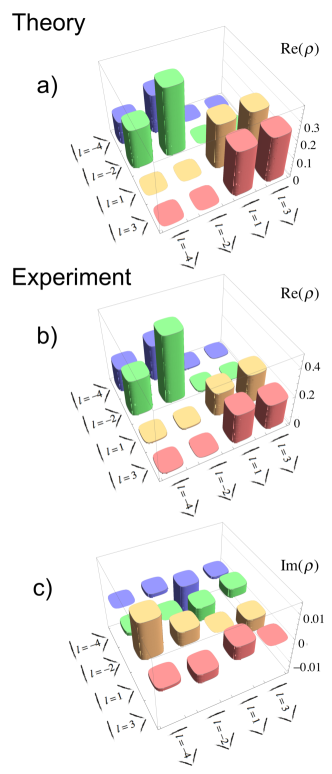
Figure 3: The performance of the duplexer is quantified by means of state tomography to measure the output density matrix in order to compare this with the intended ideal output given by Eq. (16). Figure a) shows the ideal density matrix for the injected states, with the phases chosen to make the density matrix real. Figure b) shows the experimentally reconstructed real part of the density matrix. Due to experimental imperfections, the imaginary part of the density matrix is small but non-zero, and is shown in c).

In order to experimentally measure our output $\hat{\rho}$, we need to make different projection measurements. If we make a set of projection measurements using a set of states $\ket{\phi}$, then the measurement $\hat{\pi}\equiv\ket{\phi}\!\bra{\phi}$ will be found with the following rate/probability

$$P=\operatorname{Tr}{(\hat{\pi}\hat{\rho})}=\Braket{\phi}{\hat{\rho}}{\phi}.$$ (11)

To measure the subspace spanned by any 2 degrees of freedom (e.g. $\ket{\ell_{1}}$ and $\ket{\ell_{2}}$) we need to make a number of projective measurements in order to reconstruct the total state $\hat{\rho}$. Projecting on the state $\Ket{\phi}=\Ket{\ell_{1}}$ or $\ket{\ell_{2}}$ will give the diagonal elements $\rho_{11}$ and $\rho_{22}$. While $\ket{\phi}\propto\ket{\ell_{1}}\pm\ket{\ell_{2}}$ will give

$$P_{\pm}=\operatorname{Tr}{(\hat{\pi}_{\pm}\hat{\rho})}=\rho_{11}+\rho_{22}\pm(\rho_{12}+\rho_{21}).$$ (12)

Now $\rho_{12}+\rho_{21}=\rho_{12}+\rho_{12}^{*}=2\Re{(\rho_{12})}$ so we can get the real part of $\rho_{12}$ from a differential measurement (to avoid miscalibration errors)

$$\Re{(\rho_{12})}=(P_{+}-P_{-})/4.$$ (13)

In order to find the imaginary part $\Im{(\rho_{12})}$, we need to measure in a 3rd basis. This is why in quantum tomography of a qubit one needs to measure in $\hat{\sigma}_{x}$, $\hat{\sigma}_{y}$, and $\hat{\sigma}_{z}$ bases, or equivalently measure the three Stokes Parameters $S_{1}$, $S_{2}$, and $S_{3}$. For this reason our measured parameters $P$ are sometimes referred to as “Qudit Stokes Parameters” Altepeter et al. (2005).

So to get the imaginary part of $\rho_{12}$, we measure $\ket{\phi}=\ket{\ell_{1}}\pm i\ket{\ell_{2}}$ and follow a similar procedure as before which gives

$$P^{\prime}_{\pm}=\operatorname{Tr}{(\hat{\pi}_{\pm}\hat{\rho})}=\rho_{11}+\rho_{22}\pm i(\rho_{12}-\rho_{21}).$$ (14)

Taking the difference of these two rates allows one to find the imaginary part of $\rho_{21}$ which is given by

$$\Im{(\rho_{12})}=(P^{\prime}_{-}-P^{\prime}_{+})/4.$$ (15)

In order to make our projection measurements, we use the standard method developed for measuring spatial modes Mair et al. (2001). The output of the bright port of our device was imaged onto an SLM with the complex conjugate of the field mode we wish to measure, encoded onto a modulated diffraction grating. We then couple the first diffraction order into single mode fiber and measure the count rate on an APD. It has been demonstrated that for such projection measurements there exists cross-talk between neighboring modes Qassim et al. (2014). In order to avoid this issue we prepared the incoherent superposition of $\ket{\psi_{1}}=1/\sqrt{4}\ket{1}+\sqrt{3/4}\ket{3}$ and $\ket{\psi_{2}}=1/\sqrt{2}(\ket{-2}+\ket{-4})$, which allows us to obtain cleaner results in our projection measurment as neighboring modes are not used. Written in matrix formation for the basis states $\ell\in\left[-4,-2,1,3\right]$ gives [via Eq. (10)]

$$\rho_{ij}=\frac{1}{8}\begin{pmatrix}2&2&0&0\\ 2&2&0&0\\ 0&0&1&\sqrt{3}\\ 0&0&\sqrt{3}&3\\ \end{pmatrix}.$$ (16)

Our results are shown in Fig. 3. The phases of our states where chosen such that $\rho$ is ideally real as shown in Fig. 3a. Our measured state, shown in Fig. 3b (c) shows the real (imaginary) part of our measure state $\rho_{m}$, which demonstrates excellent agreement with our intended state. Using the standard measure of fidelity defined as Jozsa (1994)

$$F(\rho,\rho_{m})\equiv\operatorname{Tr}\left[\sqrt{\rho}\rho_{m}\sqrt{\rho}\right]^{1/2},$$ (17)

we find our measured state has a fidelity of 0.9880.

In conclusion, we have experimentally demonstrated the use of a protocol for multiplexing even and odd spatial modes of light with OAM states. We have shown that this multiplexing scheme can generate general incoherent mixes of states in a simple and deterministic way. The fact that this protocol works at low or single photon levels makes this scheme a promising tool for use in quantum information tasks.

V Acknowledgements

The authors thank E. Karimi for excellent discussion. RWB acknowledges funding from the Canada Excellence Research Chairs program. OSML acknowledges support from the Consejo Nacional de Ciencia y Tecnología (CONACyT), the Secretaría de Educación Pública (SEP), and the Gobierno de Mexico.

References

- Allen et al. (1992) L. Allen, Marco Beijersbergen, R. Spreeuw, and J. P. Woerdman, “Orbital angular momentum of light and the transformation of Laguerre-Gaussian laser modes,” Phys. Rev. A 45, 8185–8189 (1992).
- Gibson et al. (2004) Graham Gibson, Johannes Courtial, Miles J Padgett, Mikhail Vasnetsov, Valeriy Pas’ko, Stephen M Barnett, and Sonja Franke-Arnold, “Free-space information transfer using light beams carrying orbital angular momentum,” Opt. Express 12, 5448 (2004).
- Wang et al. (2012) Jian Wang, Jeng-Yuan Yang, Irfan M. Fazal, Nisar Ahmed, Yan Yan, Hao Huang, Yongxiong Ren, Yang Yue, Samuel Dolinar, Moshe Tur, and Alan E Wilner, “Terabit free-space data transmission employing orbital angular momentum multiplexing,” Nat. Photonics 6, 488–496 (2012).
- Tamburini et al. (2012) Fabrizio Tamburini, Elettra Mari, Anna Sponselli, Bo Thidé, Antonio Bianchini, and Filippo Romanato, “Encoding many channels on the same frequency through radio vorticity: first experimental test,” New J. Phys. 14, 033001 (2012).
- Mirhosseini et al. (2015) Mohammad Mirhosseini, Omar S. Magaña Loaiza, Malcolm N. O’Sullivan, Brandon Rodenburg, Mehul Malik, Daniel J. Gauthier, and Robert W. Boyd, “High-dimensional quantum cryptography with twisted light,” New J. Phys. 17, 033033 (2015).
- Mair et al. (2001) A Mair, A Vaziri, G Weihs, and Anton Zeilinger, “Entanglement of the orbital angular momentum states of photons.” Nat. 412, 313–6 (2001).
- Molina-Terriza et al. (2007) Gabriel Molina-Terriza, Juan P. Torres, and Lluis Torner, “Twisted photons,” Nat. Physics 3, 305–310 (2007).
- Nagali et al. (2009) Eleonora Nagali, Fabio Sciarrino, Francesco De Martini, Lorenzo Marrucci, Bruno Piccirillo, Ebrahim Karimi, and Enrico Santamato, “Quantum Information Transfer from Spin to Orbital Angular Momentum of Photons,” Phys. Rev. Lett. 103, 013601 (2009).
- Potoček et al. (2015) Václav Potoček, Filippo M. Miatto, Mohammad Mirhosseini, Omar S. Magaña-Loaiza, Andreas C. Liapis, Daniel K. L. Oi, Robert W. Boyd, and John Jeffers, “Quantum Hilbert Hotel,” Phys. Rev. Lett. 115, 160505 (2015).
- García-Escartín and Chamorro-Posada (2008) Juan García-Escartín and Pedro Chamorro-Posada, “Quantum multiplexing with the orbital angular momentum of light,” Phys. Rev. A 78, 062320 (2008).
- Leach et al. (2002) Jonathan Leach, Miles Padgett, Stephen Barnett, Sonja Franke-Arnold, and Johannes Courtial, “Measuring the Orbital Angular Momentum of a Single Photon,” Phys. Rev. Lett. 88, 257901 (2002).
- Gatto et al. (2011) Alberto Gatto, Matteo Tacca, Paolo Martelli, Pierpaolo Boffi, and Mario Martinelli, “Free-space orbital angular momentum division multiplexing with Bessel beams,” Journal of Optics 13, 064018 (2011).
- Martelli et al. (2011) P. Martelli, A. Gatto, P. Boffi, and M. Martinelli, “Free-space optical transmission with orbital angular momentum division multiplexing,” Electronics Letters 47, 972 (2011).
- Altepeter et al. (2005) Joseph B Altepeter, Evan R Jeffrey, and Paul G Kwiat, “Photonic State Tomography,” Advances In Atomic, Molecular, and Optical Physics 52, 105–159 (2005).
- Qassim et al. (2014) Hammam Qassim, Filippo M. Miatto, Juan P. Torres, Miles J. Padgett, Ebrahim Karimi, and Robert W. Boyd, “Limitations to the determination of a Laguerre–Gauss spectrum via projective, phase-flattening measurement,” J. Opt. Soc. Am. B 31, A20 (2014).
- Jozsa (1994) Richard Jozsa, “Fidelity for Mixed Quantum States,” J. Mod. Opt. 41, 2315–2323 (1994).