Prediction-Based Task Assignment in Spatial Crowdsourcing (Technical Report)

Abstract

With the rapid advancement of mobile devices and crowdsourcing platforms, spatial crowdsourcing has attracted much attention from various research communities. A spatial crowdsourcing system periodically matches a number of location-based workers with nearby spatial tasks (e.g., taking photos or videos at some specific locations). Previous studies on spatial crowdsourcing focus on task assignment strategies that maximize an assignment score based solely on the available information about workers/tasks at the time of assignment. These strategies can only achieve local optimality by neglecting the workers/tasks that may join the system in a future time. In contrast, in this paper, we aim to improve the global assignment, by considering both present and future (via predictions) workers/tasks. In particular, we formalize a new optimization problem, namely maximum quality task assignment (MQA). The optimization objective of MQA is to maximize a global assignment quality score, under a traveling budget constraint. To tackle this problem, we design an effective grid-based prediction method to estimate the spatial distributions of workers/tasks in the future, and then utilize the predictions to assign workers to tasks at any given time instance. We prove that the MQA problem is NP-hard, and thus intractable. Therefore, we propose efficient heuristics to tackle the MQA problem, including MQA greedy and MQA divide-and-conquer approaches, which can efficiently assign workers to spatial tasks with high quality scores and low budget consumptions. Through extensive experiments, we demonstrate the efficiency and effectiveness of our approaches on both real and synthetic datasets.

I Introduction

Mobile devices not only bring convenience to our daily life, but also enable people to easily perform location-based tasks in their vicinity, such as taking photos/videos (e.g., street view of Google Maps [2]), reporting traffic conditions (e.g., Waze [4]), and identifying the status of display shelves at neighborhood stores (e.g., Gigwalk [1]). Recently, to exploit these phenomena, a new framework, namely spatial crowdsourcing [17], for requesting workers to perform spatial tasks, has drawn much attention from both academia (e.g., MediaQ [18]) and industry (e.g., TaskRabbit [3]). A typical spatial crowdsourcing system (e.g., gMission [7]) utilizes a number of dynamically moving workers to accomplish spatial tasks (e.g., taking photos/videos), which requires workers to physically go to the specified locations to complete these tasks.

We first provide the following motivating example.

Example 1 (The Spatial Crowdsourcing Problem with Multiple Time Instances) Consider a scenario of spatial crowdsourcing in Figure 1, where spatial tasks, $t_{1}$ $\sim$ $t_{3}$, are represented by red circles, and workers, $w_{1}$ $\sim$ $w_{3}$, are denoted by blue triangles. In particular, Figure 1() shows a worker, $w_{1}$, and two tasks, $t_{1}$ and $t_{2}$, which join the system at a timestamp $p$ (denoted by markers with solid border). Figure 1(a) depicts two more workers, $w_{2}$ and $w_{3}$, and one more task, $t_{3}$, which arrive at the system at a future timestamp $(p+1)$ (denoted by markers with the dashed border).

Each worker $w_{i}$ ($1\leq i\leq 3$) has a particular expertise to perform different types of spatial tasks $t_{j}$ ($1\leq j\leq 3$). Thus, we assume that the competence of a worker $w_{i}$ to perform task $t_{j}$ can be captured by a quality score $q_{ij}$ (as shown in Table I). Furthermore, each worker, $w_{i}$, is provided with some reward (e.g., monetary or points) to cover the traveling cost from $w_{i}$ to $t_{j}$, which is proportional to the traveling distance, $dist(w_{i},t_{j})$ (as depicted in Table I), where $dist(x,y)$ is a distance function from $x$ to $y$. Thus, workers are persuaded to perform tasks even if they are far away from the tasks’ locations, which improves the task completion rate, especially for workers/tasks with unbalanced location distributions.

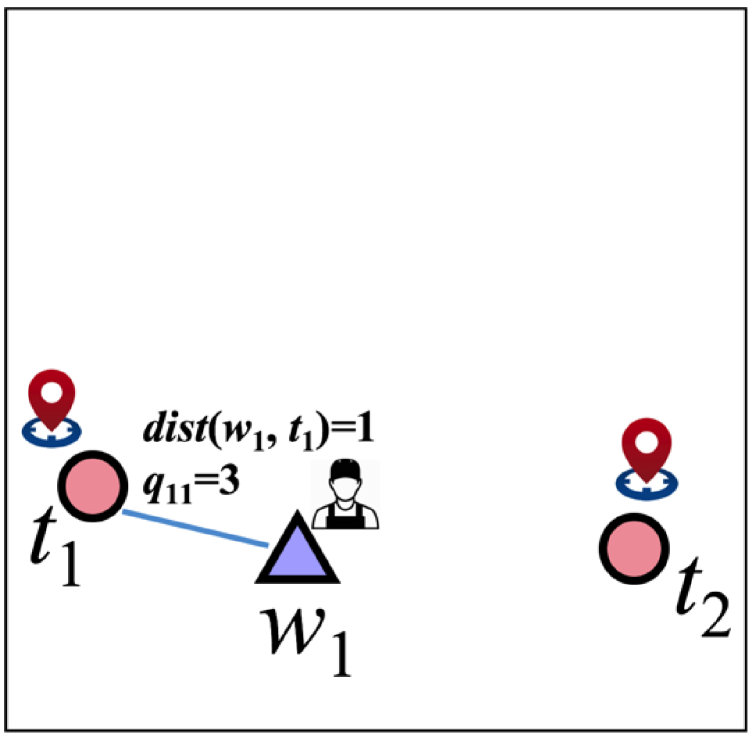
() assignment at timestamp $p$

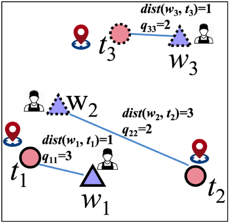
(a) assignment at timestamp $(p+1)$

Figure 1: Locally Optimal Worker-and-Task Assignments in the Spatial Crowdsourcing System.

Given a maximum reward budget at each time instance, a spatial crowdsourcing problem is to assign workers to tasks at both current and future timestamps, $p$ and $(p+1)$, respectively, such that the overall quality score of assignments is maximized while the reward for workers is under an allocated budget.

In Example 1, the traditional spatial crowdsourcing approaches [9, 18] considered the worker-and-task assignments only based on workers/tasks that are available in the system at each time instance. For example, in the first time instance, $p$, of Figure 1(), only $t_{1}$, $t_{2}$, and $w_{1}$ exist. Therefore, we assign worker $w_{1}$ to task $t_{1}$ (rather than task $t_{2}$), since it holds that $dist(w_{1},t_{1})<dist(w_{1},t_{2})$ and $q_{11}>q_{12}$ (i.e., worker $w_{1}$ can accomplish task $t_{1}$ with lower budget consumption and higher quality, compared with task $t_{2}$, as given in Table I). Next, in the second time instance of Figure 1(a), two new tasks, $t_{2}$ and $t_{3}$, and two new workers, $w_{2}$ and $w_{3}$, become available in the system at timestamp $(p+1)$. Traditional spatial crowdsourcing approaches would create assignment pairs $\langle w_{2},t_{2}\rangle$ and $\langle w_{3},t_{3}\rangle$ at this time instance (see lines in Figure 1(a)). As a result, such an assignment strategy at two separate time instances leads to the overall traveling cost 5 $(=1+3+1)$ and overall quality score 7 $(=3+2+2)$.

Note that the assignment strategy above does not take into account future workers/tasks that may join the system at a later time instance. In [17], it is shown that an optimal assignment strategy exists for a single time instance but this local optimality may not yield a global optimal assignment across all time instances. In our running example, at timestamp $p$, a clairvoyant algorithm that knows the future workers/tasks that arrive at timestamp $(p+1)$, may provide a better global assignment strategy (i.e., with lower overall traveling cost and higher overall quality score). Based on this observation, in this paper, we will formulate a new optimization problem, namely maximum quality task assignment (MQA) with the goal of assigning moving workers to spatial tasks under a budget constraint to achieve a better global assignment across multiple time instances.

TABLE I: Distances and Quality Scores of Worker-and-Task Pairs

worker-and-task pair, $\langle w_{i},t_{j}\rangle$	distance, $dist(w_{i},t_{j})$	quality score, $q_{ij}$
$\langle w_{1},t_{1}\rangle$	1	3
$\langle w_{1},t_{2}\rangle$	2	2
$\langle w_{1},t_{3}\rangle$	4	2
$\langle w_{2},t_{1}\rangle$	1	4
$\langle w_{2},t_{2}\rangle$	3	2
$\langle w_{2},t_{3}\rangle$	2	1
$\langle w_{3},t_{1}\rangle$	5	2
$\langle w_{3},t_{2}\rangle$	3	1
$\langle w_{3},t_{3}\rangle$	1	2

Example 2 (The Maximum Quality Task Assignment Problem) In the example of Figure 1, the MQA problem is to maximize the overall quality score of assignments under traveling cost budget constraints across multiple time instances. As shown in Figure 2, at timestamp $p$, we can have the prediction-based assignments: $\langle w_{2},t_{1}\rangle$, $\langle w_{1},t_{2}\rangle$, and $\langle w_{3},t_{3}\rangle$, which can achieve a better global assignment with smaller traveling cost $4$ $(=1+2+1)$ and higher quality score $8$ $(=4+2+2)$, compared to locally optimal assignments (without prediction) in Figure 1 with the traveling cost, $5$, and the quality score $7$.

As shown in [17] and from the example above, we can see that even an optimal local assignment based on the currently available tasks/workers at each time instance may not lead to a global optimal solution. In [17] , some heuristics based on past worker/task distributions (e.g., based on location entropy) were proposed to address this challenge. Here, instead, we strive to predict/estimate future task/worker distributions to provide a better global assignment strategy. Moreover, in [17], the objective was to maximize the number of assigned tasks without considering the traveling budget constraint and the quality score of task assignment. In contrast, the optimization objective of MQA is to maximize the assignment quality score under budget constraints.

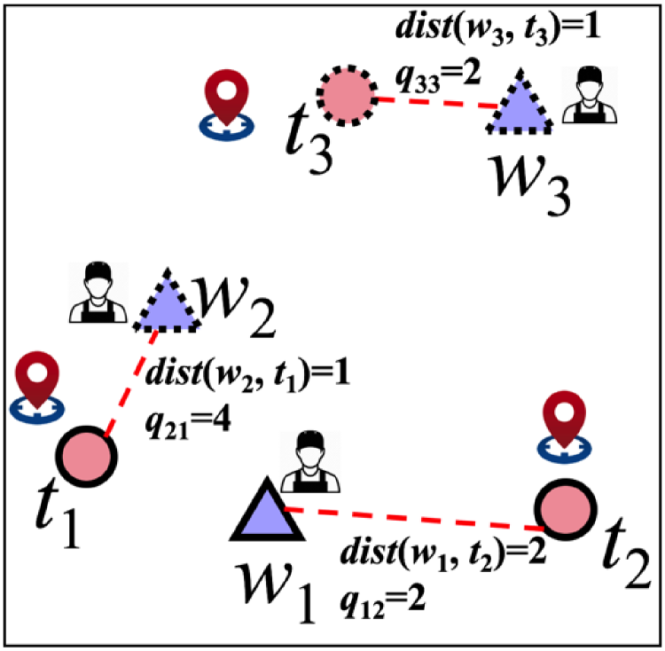
Figure 2: Globally Optimal Assignments for the Maximum Quality Task Assignment (MQA) Problem.

Different from prior studies in spatial crowdsourcing, the MQA problem requires designing an accurate prediction approach for estimating future location distributions of tasks and workers (and the quality distributions of worker-and-task assignment pairs as well), and considering the assignments over the estimated location/quality variables of future tasks/workers, which is quite challenging. Furthermore, in this paper, we prove that the MQA problem is NP-hard for any given time instance, by reducing it from the 0-1 Knapsack problem [25]. As a result, the MQA problem is not tractable. Therefore, in order to efficiently tackle the MQA problem, we will propose effective heuristics, including MQA greedy and MQA divide-and-conquer approaches, over both current and predicted workers/tasks, which can efficiently compute a better global assignment with high quality scores under the budget constraints.

Specifically, we make the following contributions.

• We formally define the maximum quality task assignment (MQA) problem in Section II. We prove that the MQA problem is NP-hard in Section II-D.

• We propose an effective grid-based prediction approach to estimate location/quality distributions/statistics for future tasks /workers in Section III.

• We design an efficient MQA greedy algorithm to iteratively select one best assignment pair each time over current/future tasks/workers in Section IV.

• We illustrate a novel MQA divide-and-conquer algorithm to recursively divide the problem into subproblems and merge assignment results in subproblems in Section V.

• We verify the effectiveness and efficiency of our proposed MQA approaches with extensive experiments on real and synthetic data sets in Section VI.

In addition to the contributions listed above, in this paper, we review previous works in spatial crowdsourcing in Section VII, and conclude in Section VIII.

II Problem Definition

II-A Dynamically Moving Workers

Definition 1

$($Dynamically Moving Workers$)$ Let $W_{p}$ $=\{w_{1},$ $w_{2},$ $...,$ $w_{n}\}$ be a set of $n$ moving workers at timestamp $p$. Each worker $w_{i}$ ($1\leq i\leq n$) is located at position $l_{i}(p)$ at timestamp $p$, and freely moves with velocity $v_{i}$.

In Definition 1, worker $w_{i}$ can dynamically move with speed $v_{i}$ in any direction. At each timestamp $p$, worker $w_{i}$ are located at positions $l_{i}(p)$. Workers can freely join or leave the spatial crowdsourcing system.

II-B Time-Constrained Spatial Tasks

Definition 2

$($Time-Constrained Spatial Tasks$)$ Let $T_{p}=\{t_{1},$ $t_{2},$ $...,$ $t_{m}\}$ be a set of time-constrained spatial tasks at timestamp $p$. Each spatial task $t_{j}$ ($1\leq j\leq m$) is located at a specific location $l_{j}$, and workers are expected to reach the location of task $t_{j}$ before the deadline $e_{j}$.

In Definition 2, a task requester creates a time-constrained spatial task $t_{j}$ (e.g., taking a photo), which requires workers to be physically at the specific location $l_{j}$ before the deadline $e_{j}$. In this paper, we assume that each spatial task can be performed by a single worker.

II-C The Maximum Quality Task Assignment Problem

In this section, we will formalize the problem of maximum quality task assignment (MQA), which assigns time-constrained spatial tasks to spatially scattered workers with the objective of maximizing the overall quality score of assignments under the traveling budget constraint.

Task Assignment Instance Set. Before we present the MQA problem, we first introduce the notion of the task assignment instance set.

Definition 3

$($Task Assignment Instance Set, $I_{p}$$)$ At timestamp $p$, given a worker set $W_{p}$ and a task set $T_{p}$, a task assignment instance set, $I_{p}$, is a set of valid worker-and-task assignment pairs in the form $\langle w_{i},t_{j}\rangle$, where each worker $w_{i}\in W_{p}$ is assigned to at most one task $t_{j}\in T_{p}$, and each task $t_{j}\in T_{p}$ is accomplished by at most one worker $w_{i}\in W_{p}$.

Intuitively, $I_{p}$ in Definition 3 is one possible (valid) worker-and-task assignment between worker set $W_{p}$ and task set $T_{p}$. A valid assignment pair $\langle w_{i},t_{j}\rangle$ is in $I_{p}$, if and only if this pair satisfies the condition that worker $w_{i}$ can reach the location $l_{j}$ of task $t_{j}$ before the deadline $e_{j}$.

The Reward of the Worker-and-Task Assignment Pair. As discussed earlier in Section I, we assume that each worker-and-task assignment pair $\langle w_{i},t_{j}\rangle$ is associated with a traveling cost, $c_{ij}$, which corresponds to the reward (e.g., monetary or points) to cover the transportation fee from $l_{i}(p)$ to $l_{j}$ (e.g., cost of gas or public transportation). Without loss of generality we assume that the reward, $c_{ij}$, is computed by: $c_{ij}=C\cdot dist(l_{i}(p),l_{j})$, where $C$ is the unit cost per mile, and $dist(l_{i}(p),$ $l_{j})$ is the distance between locations of worker $w_{i}$ and task $t_{j}$. For simplicity, we will use the Euclidean distance function $dist(l_{i}(p),$ $l_{j})$ in this paper.

The Quality Score of the Worker-and-Task Assignment Pair. Each worker-and-task assignment pair $\langle w_{i},t_{j}\rangle$ is also associated with a quality score, denoted as $q_{ij}$ ($\in[0,1]$), which indicates the quality of the task $t_{j}$ that is completed by worker $w_{i}$. Due to different types of tasks with various difficulty levels (e.g., taking photos vs. repairing houses) and different expertise or competence of workers in performing tasks, we assume that different worker-and-task pairs $\langle w_{i},t_{j}\rangle$ may be associated with diverse quality scores $q_{ij}$.

The MQA Problem. Next, we provide the definition of our maximum quality task assignment (MQA) problem.

Definition 4

$($Maximum Quality Task Assignment (MQA) $)$ Given a set of time instances $P$ and a maximum reward budget $B$ for each time instance, the problem of maximum quality task assignment (MQA) is to assign the available workers in $W_{p}$ to tasks in $T_{p}$ to provide a task assignment instance set, $I_{p}$, at timestamp $p\in P$, such that:

1. at any timestamp $p\in P$, each worker $w_{i}\in W_{p}$ is assigned to at most one spatial task $t_{j}\in T_{p}$ such that his/her arrival time at location $l_{j}$ is before deadline $e_{j}$;

2. at timestamp $p\in P$, the total reward (i.e., the traveling cost) of all the assigned workers does not exceed budget $B$, that is, $\sum_{\forall\langle w_{i},t_{j}\rangle\in I_{p}}c_{ij}$ $\leq B$; and

3. the overall quality score of the assigned tasks of all timestamps in $P$ is maximized, that is,

   $$\text{maximize }\sum_{\forall p\in P}\sum_{\forall\langle w_{i},t_{j}\rangle\in I_{p}}q_{ij}.\vspace{-4ex}$$ (1)

Intuitively, the MQA problem (given in Definition 4) assigns workers to tasks at multiple time instances in $P$, such that (1) at each time instance, an assignment pair $\langle w_{i},t_{j}\rangle$ is valid (i.e., satisfying the time constraints, $e_{j}$); (2) at each time instance, the total reward of assignment pairs is less than or equal to the maximum budget $B$; and (3) the overall quality score of assignments of all the time instances is maximized.

As discussed earlier in Section I, it may not be globally optimal to simply optimize the assignments at each individual time instance separately. The MQA approaches aim to provide a better global assignment by taking into account tasks/workers not only at the current timestamp $p$, but also at the future timestamp $(p+i)\in P$.

Table II summarizes the commonly used symbols.

TABLE II: Symbols and Descriptions.

Symbol	Description
$T_{p}$	a set of $m$ time-constrained spatial tasks $t_{j}$ at timestamp $p$
$W_{p}$	a set of $n$ dynamically moving workers $w_{i}$ at timestamp $p$
$\hat{w_{i}}$ (or $\hat{t_{j}}$)	the predicted worker (or task)
$\tilde{w_{i}}$ (or $\tilde{t_{j}}$)	the worker (or task) in either current or next time instance
$I_{p}$	the task assignment instance set at timestamp $p$
$e_{j}$	the deadline of arriving at the location of task $t_{j}$
$l_{i}(p)$	the position of worker $w_{i}$ at timestamp $p$
$l_{j}$	the position of task $t_{j}$
$v_{i}$	the velocity of worker $w_{i}$
$c_{ij}$	the traveling cost from the location of worker $w_{i}$ to that of task $t_{j}$
$q_{ij}$	the quality score of assigning worker $w_{i}$ to perform task $t_{j}$
$B$	the maximum reward budget (i.e., traveling cost) at each time instance
$C$	the unit price of the traveling cost by workers
$P$	a set of time instances
$w$	the size of the sliding window to do the prediction

II-D Hardness of the MQA Problem

In order to give a sense on the size of the solution space, with $n$ dynamically moving workers and $m$ time-constrained spatial tasks, in the worst case, there are an exponential number of possible worker-and-task assignment strategies, which leads to high time complexity (i.e., $O((m+1)^{n})$). Then, we prove that the MQA problem is NP-hard, by reducing it from a well-known NP-hard problem, 0-1 Knapsack problem [25].

Lemma II.1

(Hardness of the MQA Problem) The maximum quality task assignment (MQA) problem is NP-hard.

Proof:

Please refer to Appendix A. ∎

From Lemma II.1, we can see that the MQA problem is NP-hard, and thus intractable. Alternatively, we will later design efficient heuristics to tackle the MQA problem and achieve better global assignment strategies.

II-E Framework

Figure 3 illustrates a general framework, namely procedure MQA_Framework, for solving the MQA problem, which assigns workers with spatial tasks at multiple time instances in $P$, based on the predicted location/quality distributions of workers/tasks.

Specifically, at timestamp $p$, we first retrieve a set, $T_{p}$, of available spatial tasks, and a set, $W_{p}$, of available workers (lines 1-3). Here, the task set $T_{p}$ (or worker set $W_{p}$) contains both tasks (or workers) that have not been assigned at the last time instance and the ones that newly arrive at the system after the last time instance (note: those workers who finished tasks in previous time instances are also treated as “new workers” that join the system, thus the workers can continuously contribute to the platform). In order to achieve better global assignments, we need to predict workers and tasks at a future timestamp $(p+1)$ that newly join the system, and obtain two sets $W_{p+1}$ and $T_{p+1}$, respectively (line 4).

Subsequently, with both current and future sets of tasks/workers (i.e., $T_{p}$/$W_{p}$ and $T_{p+1}$/$W_{p+1}$, respectively), we can apply our proposed algorithms in this paper (including MQA greedy and MQA divide-and-conquer), and retrieve better assignment pairs in assignment instance set $I_{p}$ (line 5). Finally, we notify each worker $w_{i}$ to do his/her task $t_{j}$ (lines 6-7).

Procedure MQA_Framework { Input: a set of time instances $P$ Output: a worker-and-task assignment strategy across the time instances in $P$ (1) for time instance $p\in P$ (2) retrieve all the available spatial tasks in set $T_{p}$ (3) retrieve all the available workers in set $W_{p}$ (4) predict new future tasks/workers in $T_{p+1}$ and $W_{p+1}$ at the next time instance (5) apply the MQA greedy or MQA divide-and-conquer approach to obtain a assignment instance set, $I_{p}$, w.r.t. $T_{p}$, $W_{p}$, $T_{p+1}$ and $W_{p+1}$ (6) for each pair $\langle w_{i},t_{j}\rangle$ in $I_{p}$ (7) inform worker $w_{i}$ to perform task $t_{j}$}

Figure 3: A Framework for Tackling the MQA Problem.

III The Grid-based Worker/Task
Prediction Approach

In order to achieve better global assignments in our MQA problem, we need to accurately predict the future status of workers/tasks that newly join the spatial crowdsourcing system. Specifically, in this section, we will introduce a grid-based worker/task prediction approach, which can efficiently and effectively estimate the number of future workers/tasks, location distributions of future workers/tasks, and quality score distributions w.r.t. future worker-and-task pairs (and their existence probabilities as well).

TABLE III: Example of Grid-Based Prediction

Cell	Previous Worker Numbers	Predicted Worker Number
$C_{1}$	[4, 3, 4]	4
$C_{2}$	[2, 3, 3]	3
$C_{3}$	[0, 1, 0]	0
$C_{4}$	[1, 1, 1]	1

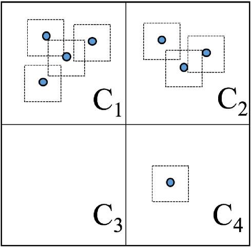
Figure 4: Example of Predicted Workers.

III-A The Grid-Based Prediction Algorithm

In this section, we discuss how to predict the number of tasks /workers, and their location distributions in a 2-dimensional data space $\mathcal{U}=[0,1]^{2}$. In particular, we consider a grid index, $\mathcal{I}$, over tasks and workers, which divides the data space $\mathcal{U}$ into $\gamma^{2}$ cells, each with the side length $1/\gamma$, where the selection of the best $\gamma$ value can be guided by a cost model in [9]. Next, we estimate the potential workers/tasks that may fall into each cell at a future timestamp, which is inferred from historical data of the most recent sliding window of size $w$.

In particular, our grid-based prediction algorithm first predicts the future numbers of workers/tasks from the latest $w$ worker/task sets in each cell, then generates possible worker (or task) samples in $W_{p+1}$ (or $T_{p+1}$) for each cell of the grid index $\mathcal{I}$.

First, we initialize a worker set $W_{p+1}$ and a task set $T_{p+1}$ at the future time instance with empty sets. Subsequently, within each cell $cell_{i}$, we can obtain its $w$ latest worker counts, $|W_{p-w+1}^{(i)}|$, $|W_{p-w+2}^{(i)}|$, …, and $|W_{p}^{(i)}|$, which form a sliding window of a time series (with size $w$). Due to the temporal correlation of worker counts in the sliding window, in this paper, we utilize the linear regression [19] over these $w$ worker counts to predict the future number, $|W_{p+1}^{(i)}|$, of workers in cell, $cell_{i}$, that newly join the system at timestamp $(p+1)$. Note that other prediction methods can be also plugged into our grid-based prediction framework, which we plan to study in our future work. Similarly, we can estimate the number, $|T_{p+1}^{(i)}|$, of tasks in $cell_{i}$ at timestamp $(p+1)$.

According to the predicted numbers of workers/tasks, we can uniformly generate $|W_{p+1}^{(i)}|$ worker samples (or $|T_{p+1}^{(i)}|$ task samples) within each cell $cell_{i}$, and add them to the predicted worker set $W_{p+1}$ (or task set $T_{p+1}$). We use sampling with replacement to generate worker/task samples, which means two samples can be generated at the same location. For the pseudo code of the MQA prediction algorithm, please refer to Appendix B.

Example 3 (The Grid-Based Prediction) Consider that a space is divided into 4 cells, $C_{1}$ to $C_{4}$, as shown in Figure 4. Based on the historical records on the number of workers in each cell $C_{i}$, we want to predict the workers that will appear in $C_{i}$ at the next time instance. Table III presents the number of workers for each cell in current time instance $p$ and previous two time instances $p-1$ and $p-2$. For example, there 4 workers at time $p-2$, 3 workers at time $p-1$ and 4 workers at time $p$ in cell $C_{1}$. Then, we predict the number of workers in cell $C_{1}$ at time $p+1$ is 4. We uniformly generate 4 worker samples. After generating predicted workers for each cell, we can capture the distribution of workers as shown in Figure 4.

Location Distributions of the Predicted Workers/Tasks. As each cell is small, from the global view, the distributions of tasks/workers in the entire space are approximately captured. However, in each cell, discrete samples may be of small sample sizes, which may lead to low prediction accuracy. For example, if the sample size is only 1, then different possible locations of this one single sample (generated in the cell) may dramatically affect our MQA assignment results.

Inspired by this, instead of using discrete samples predicted, in this paper, we will alternatively consider continuous probability density function (pdf) for location distributions of workers/tasks. Specifically, we apply the kernel density estimation over samples in each cell to describe the distributions of samples’ locations. That is, centered at each sample $s_{i}$ generated in $cell_{i}$, we can obtain the continuous pdf function of this worker/task sample, $f(x)=\prod_{r=1}^{2}\left(\frac{1}{h_{r}}K\left(\frac{x[r]-s[r]}{h_{r}}\right)\right)$, where $h_{r}$ ($\in(0,1)$) is the bandwidth on the $r$-th dimension, and function $K(\cdot)$ is a uniform kernel function [14], given by $K(u)=\frac{1}{2}\cdot\mathbf{1}{(|u|\leq 1)}$. Here, $\mathbf{1}{(|u|\leq 1)}=1$, when $|u|\leq 1$ holds. Note that the choice of the kernel function is not significant for approximation results [14], thus, in this paper, we use uniform kernel function $K(\cdot)$. From the pdf function $f(x)$ of each sample $s_{i}\in cell_{i}$, each dimension $r$ can be bounded by an interval $[s_{i}[r]-h_{r},s_{i}[r]+h_{r}]$.

Typically, in the literature [14], we set $h_{r}=\hat{\sigma}C_{v}(k)n^{-1/(2v+1)}$, where $\hat{\sigma}$ is the standard deviation of samples (derived from current worker/task statistics), $v$ is the order of the kernel ($v$ is set to 2 here), and $C_{v}(k)=1.8431$ ($=2\left(\frac{\pi^{1/2}(v!)^{3}R(k)}{2v(2v)!k_{v}^{2}(k)}\right)^{1/(2v+1)}$, for $k_{v}(k)=1/3,R(k)=1/2$ with Uniform kernel functions).

III-B Statistics of the Predicted Workers/Tasks

For the ease of the presentation, in this paper, we denote those future workers $w_{i}$ and tasks $t_{j}$ that are predicted as $\widehat{w_{i}}$ and $\widehat{t_{j}}$, respectively.

Due to the predicted future workers/tasks, in our PB-SC problem, we need to consider worker-and-task assignment pairs that may involve predicted workers/tasks. That is, we have 3 cases, $\langle\widehat{w_{i}},t_{j}\rangle$, $\langle w_{i},\widehat{t_{j}}\rangle$, and $\langle\widehat{w_{i}},\widehat{t_{j}}\rangle$, where $\widehat{w_{i}}$ and $\widehat{t_{j}}$ are the predicted worker and task samples, respectively, following uniform distributions represented by kernel functions $K(\cdot)$ (as mentioned in Section III-A).

Due to the existence of these predicted workers/tasks, the traveling costs and the quality scores of assignment pairs now become random variables (rather than fixed values). In this section, we will discuss how to obtain statistics (e.g., mean and variance) of traveling costs, quality scores, and confidences, associated with assignment pairs.

The Traveling Cost of Pairs with the Predicted Workers/Tasks. The traveling cost, $\widehat{c_{ij}}$, of worker-and-task pairs involving the predicted workers/tasks (i.e., $\langle\widehat{w_{i}},t_{j}\rangle$, $\langle w_{i},\widehat{t_{j}}\rangle$, or $\langle\widehat{w_{i}},\widehat{t_{j}}\rangle$) can be given by $C\cdot dist(\widehat{w_{i}},t_{j})$, $C\cdot dist(w_{i},\widehat{t_{j}})$, or $C\cdot dist(\widehat{w_{i}},\widehat{t_{j}})$, respectively.

We discuss the general case of computing statistics of variable $\widehat{c_{ij}}=C\cdot dist(\widehat{w_{i}},\widehat{t_{j}})$. Since it is nontrivial to calculate the statistics of the Euclidean distance between variables $\widehat{w_{i}}$ and $\widehat{t_{j}}$, we alternatively consider statistics (mean and variance) of the squared Euclidean distance variable $Z^{2}=dist^{2}(\widehat{w_{i}},\widehat{t_{j}})$ ($=\sum_{r=1}^{2}(\widehat{w_{i}}[r]-\widehat{t_{j}}[r])^{2}$), where $\widehat{w_{i}}$ and $\widehat{t_{j}}$ are two variables uniformly residing in a 2D space.

The Computation of Mean $E(Z^{2})$. Let variable $Z_{r}=\widehat{w_{i}}[r]-\widehat{t_{j}}[r]$, for $r=1,2$, whose mean $E(Z_{r})$ and variance $Var(Z_{r})$ can be easily computed (i.e., $E(Z_{r})=s_{i}[r]-s_{j}[r]$ and $Var(Z_{r})=\frac{(h_{r}(\widehat{w_{i}}[r]))^{2}+(h_{r}(\widehat{t_{j}}[r]))^{2}}{3}$ respectively).

Then, we have $Z^{2}=Z_{1}^{2}+Z_{2}^{2}$. Thus, the mean $E(Z^{2})$ can be given by:

$$E(Z^{2})=E(Z_{1}^{2})+E(Z_{2}^{2}).$$ (2)

The Computation of Variance $Var(Z^{2})$. Moreover, for variance $Var(Z^{2})$, it holds that:

$$Var(Z^{2}) = E(Z^{4})-(E(Z^{2}))^{2}$$

$$= E((Z_{1}^{2}+Z_{2}^{2})^{2})-(E(Z^{2}))^{2}$$

$$= E(Z_{1}^{4})+2\cdot E(Z_{1}^{2})\cdot E(Z_{2}^{2})+E(Z_{2}^{4})-(E(Z^{2}))^{2}.$$

From Eqs. (2) and (III-B) above, the remaining issues are to compute $E(Z_{r}^{2})$ and $E(Z_{r}^{4})$ (for $r=1,2$).

The Computation of $E(Z_{r}^{2})$. For $E(Z_{r}^{2})$, since $Z_{r}=\widehat{w_{i}}[r]-\widehat{t_{j}}[r]$, we have:

$$E(Z_{r}^{2}) = Var(Z_{r})+(E(Z_{r}))^{2}$$

$$= Var(\widehat{w_{i}}[r])+Var(\widehat{t_{j}}[r])+(E(\widehat{w_{i}}[r])-E(\widehat{t_{j}}[r]))^{2}.$$

The Computation of $E(Z_{r}^{4})$. For $E(Z_{r}^{4})$, we can derive that:

$$E(Z_{r}^{4}) = E((\widehat{w_{i}}[r]-\widehat{t_{j}}[r])^{4})$$ (5)

$$= E(\widehat{w_{i}}[r]^{4})-4\cdot E(\widehat{w_{i}}[r]^{3})\cdot E(\widehat{t_{j}}[r])$$

$$+6\cdot E(\widehat{w_{i}}[r]^{2})\cdot E(\widehat{t_{j}}[r]^{2})-4\cdot E(\widehat{w_{i}}[r])\cdot E(\widehat{t_{j}}[r]^{3})$$

$$+E(\widehat{t_{j}}[r]^{4}).$$

In Eq. (5), variable $\widehat{w_{i}}[r]$ follows the uniform distribution within bound $[lb\_w,ub\_w]$ (for the $r$-th dimension of uniform kernel function $K(\cdot)$ in Section III-A). We can thus infer that:

$$E(\widehat{w_{i}}[r]^{4}) = \int_{lb\_w}^{ub\_w}x^{4}\frac{1}{ub\_w-lb\_w}dx=\frac{ub\_w^{5}-lb\_w^{5}}{5(ub\_w-lb\_w)},$$

$$E(\widehat{w_{i}}[r]^{3}) = \int_{lb\_w}^{ub\_w}x^{3}\frac{1}{ub\_w-lb\_w}dx=\frac{ub\_w^{4}-lb\_w^{4}}{4(ub\_w-lb\_w)},$$

$$E(\widehat{w_{i}}[r]^{2}) = \int_{lb\_w}^{ub\_w}x^{2}\frac{1}{ub\_w-lb\_w}dx=\frac{ub\_w^{3}-lb\_w^{3}}{3(ub\_w-lb\_w)},$$

where $[lb\_w,ub\_w]=[s_{i}[r]-h_{r}(\widehat{w_{i}}[r]),s_{i}[r]+h_{r}(\widehat{w_{i}}[r])]$.

Similarly, we can also obtain $E(\widehat{t_{j}}[r]^{4})$, $E(\widehat{t_{j}}[r]^{3})$, and $E(\widehat{t_{j}}[r]^{2})$ for task $\widehat{t_{j}}[r]$. We omit it here.

This way, by substituting Eqs. (III-B) and (5) into Eqs. (2) and (III-B), we can obtain mean $E(Z^{2})$ and variance $Var(Z^{2})$ of the squared Euclidean distance between two Uniform distributions.

Quality Scores of Pairs with the Predicted Workers/Tasks. We consider the three cases to compute statistics of quality score distributions.

Case 1: $\langle\widehat{w_{i}},t_{j}\rangle$. In this case, at the current timestamp $p$, we can obtain all the $n_{i}$ workers $w_{i}$ that can reach task $t_{j}$. Then, we use quality scores, $q_{ij}$, of their corresponding worker-and-task pairs $\langle w_{i},t_{j}\rangle$ as samples (each with probability $1/n_{i}$), which can describe/estimate future distributions of quality scores. Correspondingly, with these samples, we can obtain mean and variance of quality scores between the predicted worker $\widehat{w_{i}}$ and the current task $t_{j}$.

Case 2: $\langle w_{i},\widehat{t_{j}}\rangle$. Similar to Case 1, we can obtain $m_{j}$ spatial tasks $t_{j}$ that can be reached by worker $w_{i}$. Then, we obtain $m_{j}$ quality score samples from valid pairs $\langle w_{i},t_{j}\rangle$ (each sample with probability $1/m_{j}$), whose mean and variance can be used to capture the quality score distribution between the current worker $w_{i}$ and a predicted task $\widehat{t_{j}}$.

Case 3: $\langle\widehat{w_{i}},\widehat{t_{j}}\rangle$. Since both worker $\widehat{w_{i}}$ and task $\widehat{t_{j}}$ have predicted distributions, we cannot directly obtain quality score distributions. Thus, our basic idea is to infer future quality scores by existing workers $w_{i}$ and tasks $t_{j}$ at the current timestamp $p$. That is, at the current time instance, we collect quality scores $q_{ij}$ of all pairs $\langle w_{i},t_{j}\rangle$ as samples, and use them to represent probabilistic distributions of quality scores of both worker $\widehat{w_{i}}$ and task $\widehat{t_{j}}$ at the future time instance.

Existence Probabilities of Pairs with the Predicted Workers/Tasks. Some assignment pairs that involve the predicted worker/task may not be valid, due to the time constraints of spatial tasks $t_{j}$ or $\widehat{t_{j}}$ (i.e., deadline $e_{j}$). Thus, we will associate each pair (with either worker or task in future) with an existence probability, $\widehat{p_{ij}}$.

For pair $\langle\widehat{w_{i}},t_{j}\rangle$, we let $\widehat{p_{ij}}=\min\{\frac{n_{i}}{|W_{p}|},1\}$, where $n_{i}$ is the number of valid workers who can reach task $t_{j}$ at the current timestamp $p$, and $|W_{p}|$ is the total number of (estimated) workers at timestamp $p$.

Similarly, for pair $\langle w_{i},\widehat{t_{j}}\rangle$, we can obtain: $\widehat{p_{ij}}=\min\{\frac{m_{j}}{|T_{p}|},1\}$, where $m_{j}$ is the number of valid tasks that worker $w_{i}$ can reach before the deadlines, and $|T_{p}|$ is the total number of (estimated) tasks at timestamp $p$.

For pair $\langle\widehat{w_{i}},\widehat{t_{j}}\rangle$, let $u_{ij}$ be the total number of valid pairs between $W_{p}$ and $T_{p}$ at timestamp $p$. Then, we can estimate the existence probability of pair $\langle\widehat{w_{i}},\widehat{t_{j}}\rangle$ by: $\widehat{p_{ij}}=\frac{u_{ij}}{|W_{p}|\cdot|T_{p}|}$.

IV The MQA Greedy Approach

In this section, we propose an efficient MQA greedy algorithm (GREEDY) to solve the MQA problem, which iteratively finds one “best” worker-and-task assignment pair, $\langle w_{i},t_{j}\rangle$, each time, with the highest increase of the quality score and under the budget constraint of high confidences. Here, in order to achieve high total quality scores, GREEDY is applied over both current and predicted future workers/tasks.

After all assignment pairs (involving current/future workers/tasks) are selected, we will only insert into the set $I_{p}$ those pairs, $\langle w_{i},t_{j}\rangle$, with both workers and tasks at current timestamp $p$ (i.e., $w_{i}\in W_{p}$ and $t_{j}\in T_{p}$).

IV-A The Comparisons of the Quality Score Increases / Traveling Cost Increases

Since MQA greedy algorithm needs to select one worker-and-task assignment pair, $\langle\tilde{w_{i}},\tilde{t_{j}}\rangle$, at a iteration with the highest increase of the total quality score, in this section, we will first formalize the increase of the quality score, $\Delta_{q}(\tilde{w_{i}},\tilde{t_{j}})$, for a pair $\langle\tilde{w_{i}},\tilde{t_{j}}\rangle$, and then compare the increases of overall quality scores between two pairs $\langle\tilde{w_{i}},\tilde{t_{j}}\rangle$ and $\langle\tilde{w_{a}},\tilde{t_{b}}\rangle$, where $\tilde{w_{i}}$, $\tilde{t_{j}}$, $\tilde{w_{a}}$, and $\tilde{t_{b}}$ can be either current or predicted workers/tasks.

The Calculation of the Quality Score Increase, $\Delta_{q}(\tilde{w_{i}},\tilde{t_{j}})$. Based on Eq. (1), the overall quality score is given by summing up all quality scores of the selected assignment pairs. Thus, when we choose a new assignment pair $\langle\tilde{w_{i}},\tilde{t_{j}}\rangle$, the increase of the quality score, $\Delta_{q}(\tilde{w_{i}},\tilde{t_{j}})$, is exactly equal to the quality score of this new pair $\langle\tilde{w_{i}},\tilde{t_{j}}\rangle$, denoted as $\tilde{q_{ij}}$. That is,

$$\Delta_{q}(\tilde{w_{i}},\tilde{t_{j}}) = \tilde{q_{ij}},$$ (6)

where $\tilde{q_{ij}}$ is a fixed value, if both $\tilde{w_{i}}$ and $\tilde{t_{j}}$ are current worker and task, respectively; otherwise, $\tilde{q_{ij}}$ is a random variable whose distribution can be given by samples discussed in Section III-B.

The Comparisons of the Quality Score Increase Between Two Pairs $\langle\tilde{w_{i}},\tilde{t_{j}}\rangle$ and $\langle\tilde{w_{a}},\tilde{t_{b}}\rangle$. Next, we discuss how to decide which worker-and-task assignment pair is better, in terms of the quality score increase, between two pairs $\langle\tilde{w_{i}},\tilde{t_{j}}\rangle$ and $\langle\tilde{w_{a}},\tilde{t_{b}}\rangle$.

Specifically, if both pairs have workers/tasks at current timestamp $p$, then the quality score increases, $\tilde{q_{ij}}$ and $\tilde{q_{ab}}$ (given in Eq. (6)), are fixed values. In this case, the pair with higher quality score increase is better.

On the other hand, in the case that either of the two pairs involves the predicted workers/tasks, their corresponding quality score increases, that is, $\tilde{q_{ij}}$ and/or $\tilde{q_{ab}}$, are random variables. To compare the two quality score increases, we can compute the probability, $Pr_{\Delta_{q}(\tilde{w_{i}},\tilde{t_{j}})}$, that pair $\langle\tilde{w_{i}},\tilde{t_{j}}\rangle$ has the increase greater than that of the other one. That is, by applying the central limit theorem (CLT) [13, 15], we have:

$$Pr_{\Delta_{q}(\tilde{w_{i}},\tilde{t_{j}})} = Pr\{\Delta_{q}(\tilde{w_{i}},\tilde{t_{j}})>\Delta_{q}(\tilde{w_{a}}\tilde{t_{b}})\}$$

$$= Pr\{\tilde{q_{ij}}>\tilde{q_{ab}}\}$$

$$= 1-Pr\{\tilde{q_{ij}}\leq\tilde{q_{ab}}\}$$

$$= 1-Pr\left\{\frac{\tilde{q_{ij}}-\tilde{q_{ab}}-(E(\tilde{q_{ij}})-E(\tilde{q_{ab}}))}{Var(\tilde{q_{ij}})+Var(\tilde{q_{ab}})}\right.$$

$$\left.\leq\frac{-(E(\tilde{q_{ij}})-E(\tilde{q_{ab}}))}{Var(\tilde{q_{ij}})+Var(\tilde{q_{ab}})}\right\}$$

$$= 1-\Phi\left(\frac{-(E(\tilde{q_{ij}})-E(\tilde{q_{ab}}))}{Var(\tilde{q_{ij}})+Var(\tilde{q_{ab}})}\right),$$

where $\Phi(\cdot)$ is the cumulative density function (cdf) of a standard normal distribution.

With Eq. (IV-A), we can compute the probability, $Pr_{\Delta_{q}(\tilde{w_{i}},\tilde{t_{j}})}$, that pair $\langle\tilde{w_{i}},\tilde{t_{j}}\rangle$ is better than (i.e., with higher score than) pair $\langle\tilde{w_{a}},\tilde{t_{b}}\rangle$. If it holds that $Pr_{\Delta_{q}(\tilde{w_{i}},\tilde{t_{j}})}>0.5$, then we say that pair $\langle\tilde{w_{i}},\tilde{t_{j}}\rangle$ is expected to have higher quality score increase; otherwise, pair $\langle\tilde{w_{a}},\tilde{t_{b}}\rangle$ has higher quality score increase.

The Comparisons of the Traveling Cost Increase Between Two Pairs $\langle\tilde{w_{i}},\tilde{t_{j}}\rangle$ and $\langle\tilde{w_{a}},\tilde{t_{b}}\rangle$. Similar to the quality score, we can also compute the probability, $Pr_{\Delta_{c}(\tilde{w_{i}},\tilde{t_{j}})}$, that the increase of the traveling cost for pair $\langle\tilde{w_{i}},\tilde{t_{j}}\rangle$ is smaller than that of pair $\langle\tilde{w_{a}},\tilde{t_{b}}\rangle$. That is, we can obtain:

$$Pr_{\Delta_{c}(\tilde{w_{i}},\tilde{t_{j}})} = Pr\{\Delta_{c}(\tilde{w_{i}},\tilde{t_{j}})\leq\Delta_{c}(\tilde{w_{a}},\tilde{t_{b}})\}$$

$$= Pr\{\tilde{c_{ij}}\leq\tilde{c_{ab}}\}$$

$$= \Phi\left(\frac{-(E(\tilde{c_{ij}})-E(\tilde{c_{ab}}))}{Var(\tilde{c_{ij}})+Var(\tilde{c_{ab}})}\right).$$

IV-B The Pruning Strategy

As discussed in Section IV-A, one straightforward method for selecting a “good” assignment pair at a iteration is as follows. We sequentially scan each valid worker-and-task pair $\langle\tilde{w_{i}},\tilde{t_{j}}\rangle$, and compare its quality score increase, $\Delta_{q}(\tilde{w_{i}},\tilde{t_{j}})$, with that of the best-so-far pair $\langle\tilde{w_{a}},\tilde{t_{b}}\rangle$, in terms of the probability $Pr_{\Delta_{q}(\tilde{w_{i}},\tilde{t_{j}})}$. If the pair $\langle\tilde{w_{i}},\tilde{t_{j}}\rangle$ expects to have higher quality score (and moreover satisfy the budget constraint), then we consider it as the new best-so-far pair.

The straightforward method mentioned above considers all possible valid assignment pairs, and computes their comparison probabilities, which requires high time complexity, that is, $O(m^{\prime}\cdot n^{\prime})$, where $m^{\prime}$ and $n^{\prime}$ are the numbers of tasks and workers at both current and future time instances, respectively. Therefore, in this section, we will propose effective pruning methods to quickly discard those false alarms of assignment pairs, with both high traveling costs and low quality scores.

Pruning with Bounds of Quality and Traveling Cost. Without loss of generality, for each pair $\langle\tilde{w_{i}},\tilde{t_{j}}\rangle$, assume that we can obtain its lower and upper bounds of the traveling cost, $\tilde{c_{ij}}$, and quality score, $\tilde{q_{ij}}$, where $\tilde{c_{ij}}$ and $\tilde{q_{ij}}$ are either fixed values (if $\tilde{w_{i}}$ and $\tilde{t_{j}}$ are worker/task at the current time instance) or random variables (if worker and/or task are from the future time instance). That is, we denote $\tilde{c_{ij}}\in[lb\_\tilde{c_{ij}},ub\_\tilde{c_{ij}}]$ and $\tilde{q_{ij}}\in[lb\_\tilde{q_{ij}},ub\_\tilde{q_{ij}}]$.

This way, in a 2D quality-and-travel-cost space, each worker-and-task assignment pair, $\langle\tilde{w_{i}},\tilde{t_{j}}\rangle$, corresponds to a rectangle, $[lb\_\tilde{q_{ij}},$ $ub\_\tilde{q_{ij}}]$ $\times[lb\_\tilde{c_{ij}},ub\_\tilde{c_{ij}}]$. Then, based on the idea of the skyline query [5], we can safely prune those pairs that are dominated by candidate pairs, in terms of the traveling cost and quality score.

Lemma IV.1

(The Dominance Pruning) Given a candidate pair $\langle\tilde{w_{a}},\tilde{t_{b}}\rangle$, a valid worker-and-task pair $\langle\tilde{w_{i}},\tilde{t_{j}}\rangle$ can be safely pruned, if and only if it holds that: (1) $ub\_\tilde{c_{ab}}<lb\_\tilde{c_{ij}}$, and (2) $lb\_\tilde{q_{ab}}>ub\_\tilde{q_{ij}}$.

Proof:

Since it holds that $\tilde{c_{ij}}\in[lb\_\tilde{c_{ij}},ub\_\tilde{c_{ij}}]$ and $\tilde{q_{ij}}\in[lb\_\tilde{q_{ij}},ub\_\tilde{q_{ij}}]$, by lemma assumptions and inequality transition, we have:

$$\tilde{c_{ab}}\leq ub\_\tilde{c_{ab}}<lb\_\tilde{c_{ij}}\leq\tilde{c_{ij}},\text{ and}$$

$$\tilde{q_{ab}}\geq lb\_\tilde{q_{ab}}>ub\_\tilde{q_{ij}}\geq\tilde{q_{ij}}.$$

As a result, we can see that, compared to pair $\langle\tilde{w_{a}},\tilde{t_{b}}\rangle$, pair $\langle\tilde{w_{i}},\tilde{t_{j}}\rangle$ has both higher traveling cost $\tilde{c_{ij}}$ and lower quality score $\tilde{q_{ij}}$. Since our GREEDY algorithm only selects one best pair each iteration (which can maximally increase the quality score and minimally increase the traveling cost), pair $\langle\tilde{w_{i}},\tilde{t_{j}}\rangle$ is definitely worse than $\langle\tilde{w_{a}},\tilde{t_{b}}\rangle$ in both quality and traveling cost dimensions, and thus can be safely pruned. ∎

Pruning with the Increase Probability. Lemma IV.1 utilizes the lower/upper bounds of the quality score and traveling cost to enable the dominance pruning. If a pair cannot be simply pruned by Lemma IV.1, we will further consider a more costly pruning method, by consider the probabilistic information.

Lemma IV.2

(The Increase Probability Pruning) Given a candidate pair $\langle\tilde{w_{a}},\tilde{t_{b}}\rangle$, a valid pair $\langle\tilde{w_{i}},\tilde{t_{j}}\rangle$ can be safely pruned, if and only if it holds that: (1) $Pr_{\Delta_{q}(\tilde{w_{i}},\tilde{t_{j}})}$ (w.r.t. $\langle\tilde{w_{a}},\tilde{t_{b}}\rangle$) is greater than 0.5, and (2) $Pr_{\Delta_{c}(\tilde{w_{i}},\tilde{t_{j}})}$ (w.r.t. candidate pair $\langle\tilde{w_{a}},\tilde{t_{b}}\rangle$) is greater than 0.5 , where $Pr_{\Delta_{q}(\tilde{w_{i}},\tilde{t_{j}})}$ and $Pr_{\Delta_{c}(\tilde{w_{i}},\tilde{t_{j}})}$ are given by Eqs. (IV-A) and (IV-A), respectively.

Intuitively, Lemma IV.2 filters out those pairs $\langle\tilde{w_{i}},\tilde{t_{j}}\rangle$ that have higher probabilities to be inferior to other candidate pairs $\langle\tilde{w_{a}},\tilde{t_{b}}\rangle$, in terms of both traveling cost and quality score.

Based on Lemmas IV.1 and IV.2, we can obtain a set, $S_{p}$, of candidate pairs that cannot be dominated by other pairs.

Selection of the Best Pair Among Candidate Pairs. Given a number of candidate pairs in set $S_{p}$, GREEDY still needs to identify one “best” pair with a high quality score and under the budget constraint. Specifically, we will first filter out those false alarms in $S_{p}$ with high traveling costs (i.e., violating the budget constraint), and then return one pair with the highest probability to have larger quality score than others in $S_{p}$.

Assume that in GREEDY, we have so far selected $L$ pairs, denoted as $\langle\tilde{w_{a}},\tilde{t_{b}}\rangle$. Then, with a new assignment pair $\langle\tilde{w_{i}},\tilde{t_{j}}\rangle\in S_{p}$, if it holds that:

$$Pr\left\{\left(\sum_{\forall\langle\tilde{w_{a}},\tilde{t_{b}}\rangle}\tilde{lb\_c_{ab}}\right)+\tilde{c_{ij}}\leq B_{max}\right\}\leq\delta,$$ (9)

then pair $\langle\tilde{w_{i}},\tilde{t_{j}}\rangle\in S_{p}$ can be safely ruled out from candidate set $S_{p}$, where $\delta$ is a user-specified confidence level that the selected assignment satisfies the budget constraint $B_{max}$ for both (remaining) current- and next- time instance budgets. Eq. (9) can be computed via CLT [13, 15].

Next, in the remaining candidate pairs in $S_{p}$, we will select one pair $\langle\tilde{w_{i}},\tilde{t_{j}}\rangle$ with the highest probability, $Pr_{q,max}(\langle\tilde{w_{i}},\tilde{t_{j}}\rangle)$, of having the largest high quality. That is, we have:

$$Pr_{q,max}(\langle\tilde{w_{i}},\tilde{t_{j}}\rangle)=\prod_{\forall\langle\tilde{w_{a}},\tilde{t_{b}}\rangle}Pr_{\Delta_{q}(\tilde{w_{i}},\tilde{t_{j}})}(\langle\tilde{w_{a}},\tilde{t_{b}}\rangle)$$ (10)

where $Pr_{\Delta_{q}(\tilde{w_{i}},\tilde{t_{j}})}(\langle\tilde{w_{a}},\tilde{t_{b}}\rangle)$ is the probability of quality score increase, compared with pair $\langle\tilde{w_{a}},\tilde{t_{b}}\rangle$, given by Eq. (IV-A).

Finally, among all the remaining candidate pairs in set $S_{p}$, we will choose the one, $\langle\tilde{w_{i}},\tilde{t_{j}}\rangle$, with the highest probability $Pr_{q,max}(\langle\tilde{w_{i}},$ $\tilde{t_{j}}\rangle)$, which will be included as a selected best assignment pair in GREEDY.

Procedure MQA_Greedy { Input: current and predicted workers $\tilde{w_{i}}$ in $W$, current and predicted tasks $\tilde{t_{j}}$ in $T$, and the maximum possible budget $B_{max}$ Output: a worker-and-task assignment instance set, $I_{p}$ (1) $I_{p}=\emptyset$; (2) obtain a list, $\mathcal{L}$, of valid worker-and-task pairs for $\tilde{w_{i}}\in W$ and $\tilde{t_{j}}\in T$ (3) for $k=1$ to $\min\{|W|,|T|\}$ (4) $S_{p}=\emptyset$; (5) for each valid assignment pair $\langle\tilde{w_{i}},\tilde{t_{j}}\rangle\in\mathcal{L}$ (6) if $\langle\tilde{w_{i}},\tilde{t_{j}}\rangle$ has $lb\_\tilde{c_{ij}}$ greater than the remaining budget, then continue; (7) if pair $\langle\tilde{w_{i}},\tilde{t_{j}}\rangle$ cannot be pruned w.r.t. $S_{p}$ by Lemma IV.1 (8) if pair $\langle\tilde{w_{i}},\tilde{t_{j}}\rangle$ cannot be pruned w.r.t. $S_{p}$ by Lemma IV.2 (9) add $\langle\tilde{w_{i}},\tilde{t_{j}}\rangle$ to $S_{p}$ (10) prune other candidate pairs in $S_{p}$ with $\langle\tilde{w_{i}},\tilde{t_{j}}\rangle$ (11) select one best assignment pair $\langle\tilde{w_{i}},\tilde{t_{j}}\rangle$ in $S_{p}$ satisfying the budget constraint $B_{max}$ in Eq. (9) and with the highest probability $Pr_{q,max}(\langle\tilde{w_{i}},\tilde{t_{j}}\rangle)$ in Eq. (10) (12) add the selected pair $\langle\tilde{w_{i}},\tilde{t_{j}}\rangle$ to $I_{p}$ (13) remove all those valid pairs $\langle\tilde{w_{i}},-\rangle$ or $\langle-,\tilde{t_{j}}\rangle$ from $\mathcal{L}$ (14) remove those worker-and-task pairs with the predicted workers/tasks from $I_{p}$ (15) return $I_{p}$}

Figure 5: The MQA Greedy Algorithm.

IV-C The MQA Greedy Algorithm

In this subsection, we propose MQA greedy algorithm, which iteratively assigns a worker to a spatial task greedily that can obtain a high the overall quality score under the budget constraint each iteration.

Figure 5 presents the pseudo code of our MQA greedy algorithm, namely MQA_Greedy, which obtains one best worker-and-task assignment pair each time over both current and predicted future workers and tasks, where the selected pair satisfies the budget constraint $B_{max}$ and has the largest quality score with high confidence, where $B_{max}$ is the available budget in both current and next time instances.

We first initialize the worker-and-task assignment instance set $I_{p}$ with an empty set (line 1). Then, we obtain a list, $\mathcal{L}$, of valid worker-and-task assignment pairs, which may involve either current or future workers/tasks, that is, $\tilde{w_{i}}\in W$ and $\tilde{t_{j}}\in T$ (line 2). Next, for each iteration, we find one best assignment pair with high quality score and low traveling cost (satisfying the budget constraint) (lines 3-13). In particular, we check each valid assignment pair $\langle\tilde{w_{i}},\tilde{t_{j}}\rangle$ in the list $\mathcal{L}$ (line 5). If this pair has the lower bound, $lb\_\tilde{c_{ij}}$, of the traveling cost greater than (the upper bound of) the remaining budget (w.r.t. $I_{p}$ and $B_{max}$), then it does not satisfy the budget constraint, and we can continue to check the next assignment pair (line 6). Then, if the pair $\langle\tilde{w_{i}},\tilde{t_{j}}\rangle$ cannot be pruned by dominance and increase probability pruning methods in Lemmas IV.1 and IV.2, respectively, then $\langle\tilde{w_{i}},\tilde{t_{j}}\rangle$ is a candidate pair, and we include in an initially empty candidate set $S_{p}$ (lines 7-9). In addition, we can also use candidate pair $\langle\tilde{w_{i}},\tilde{t_{j}}\rangle$ to prune other pairs in set $S_{p}$ (line 10). After that, we can insert the best pair from the candidate set $S_{p}$ into set $I_{p}$ (lines 11-12), such that the budget constraint $B_{max}$ is satisfied in Eq. (9) and the probability $Pr_{q,max}(\langle\tilde{w_{i}},\tilde{t_{j}}\rangle)$ in Eq. (10) is maximized. Since each worker can be assigned with at most one task and each task is accomplished by at most one worker, we remove those valid pairs from $\mathcal{L}$ that contains either worker $\tilde{w_{i}}$ or task $\tilde{t_{j}}$ (line 13). Finally, we remove those worker-and-task pairs involving future workers/tasks from $I_{p}$, and return the set $I_{p}$ as the solution of the MQA greedy algorithm (lines 14-15).

V The MQA Divide-and-Conquer Approach

In this section, we propose an efficient MQA divide-and-conquer algorithm (D&C), which partitions the MQA problem into $g$ subproblems, recursively conquers the subproblems, and merges assignment results from subproblems. In this paper, we will divide the MQA problem with $m^{\prime}$ current/future tasks into $g$ subproblems, each involving $\lceil m^{\prime}/g\rceil$ tasks. The D&C process continues, until the subproblem sizes become 1 (i.e., with one single spatial task in subproblems, which can be easily solved by GREEDY). We will later discuss how to utilize a cost model to estimate the best $g$ value that can achieve low MQA processing cost.

V-A The Decomposition of the MQA Problem

Decomposing the MQA Problem. Specifically, assume that the original MQA problem involves $m^{\prime}$ current/future spatial tasks for both current and next time instances. Our goal is to divide this problem into $g$ subproblems $M_{s}$ (for $1\leq s\leq g$), such that each subproblem $M_{s}$ involves a disjoint subgroup of $\lceil m^{\prime}/g\rceil$ spatial tasks, $\tilde{t_{j}}$, each of which is associated with potentially valid worker(s) $\tilde{w_{i}}$ (i.e., with valid worker-and-task assignment pairs $\langle\tilde{w_{i}},\tilde{t_{j}}\rangle$).

After the decomposition, each subproblem $M_{s}$ contains all valid pairs, $\langle\tilde{w_{i}},\tilde{t_{j}}\rangle$, w.r.t. the decomposed $\lceil m^{\prime}/g\rceil$ tasks. Since tasks in different subproblems may be reachable by the same workers, different subproblems may involve the same (conflicting) workers, whose conflictions should be resolved when we merge solutions (the selected assignment pairs) to these subproblems (as discussed in Section V-B).

Example 4 (The MQA Problem Decomposition) Figure 6 shows an example of decomposing the MQA problem (as shown in Figure 6()) into 3 subproblems (as depicted in Figure 6(a)), where each subproblem contains one single spatial task (i.e., subproblem size = 1), associated with its related valid workers. Here, the dashed border indicates the predicted future workers (i.e., $w_{4}$ and $w_{5}$) or task (i.e., $t_{3}$). In this example, the first subproblem in Figure 6(a) contains task $t_{1}$, which can be reached by workers $w_{1}$ and $w_{4}$. Different tasks may have conflicting workers, for example, tasks $t_{1}$ and $t_{2}$ from subproblems $M_{1}$ and $M_{2}$, respectively, share the same (conflicting) worker $w_{1}$.

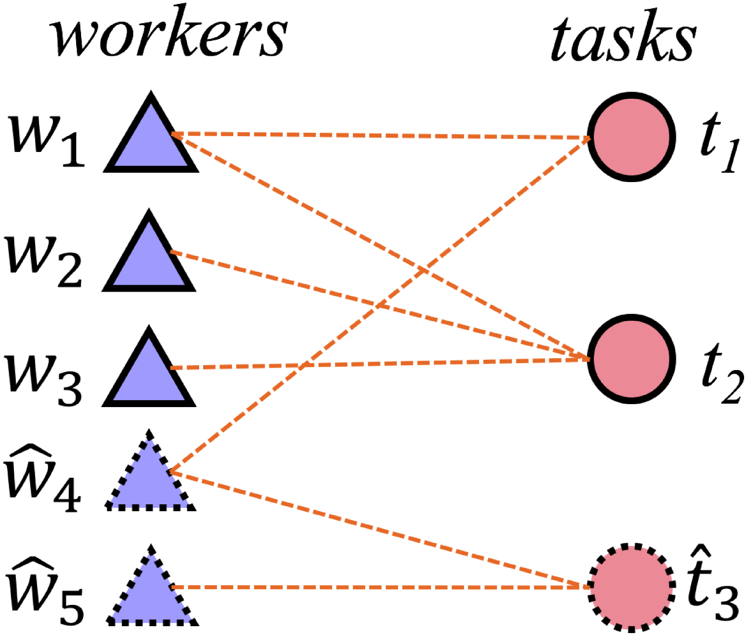
() The MQA Problem

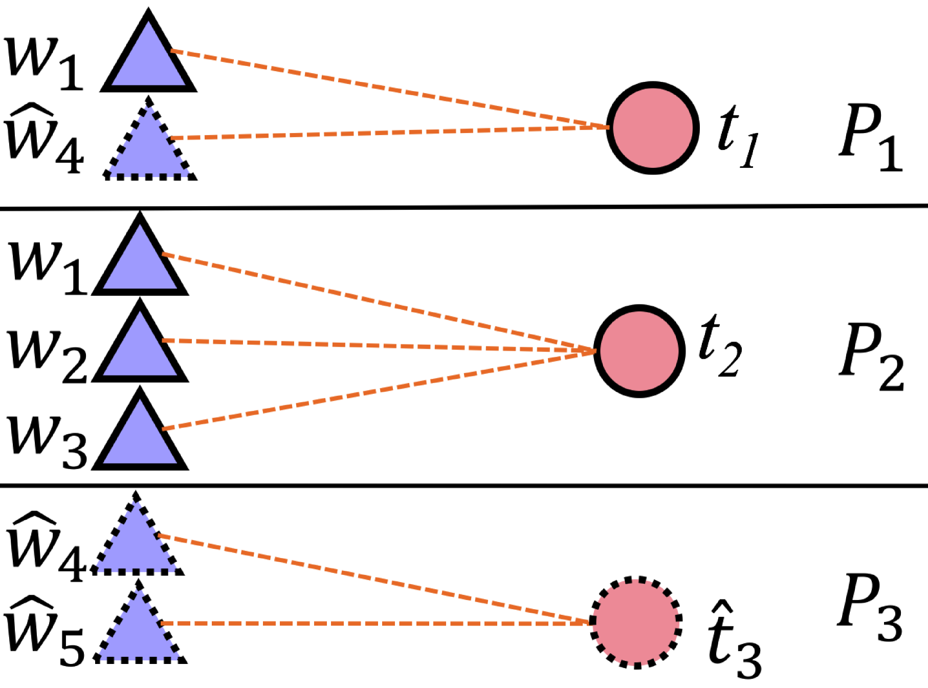
(a) The Decomposed Subproblems

Figure 6: Illustration of Decomposing the MQA Problem.

The MQA Decomposition Algorithm. Figure 7 illustrates the pseudo code of our MQA decomposition algorithm, namely MQA_Decomposition, which decomposes the MQA problem (with $m^{\prime}$ tasks), and returns $g$ MQA subproblems, $M_{s}$ (each having $\lceil m^{\prime}/g\rceil$ tasks).

Specifically, we first initialize $g$ empty subproblems, $M_{s}$, where $1\leq s\leq g$ (lines 1-2). Then, we find all valid worker-and-task assignment pairs $\langle\tilde{w_{i}},\tilde{t_{j}}\rangle$ for both current and predicted workers/tasks in sets $W$ and $T$, respectively (line 3).

Next, we want to iteratively retrieve $g$ subproblems, $M_{s}$, from the original MQA problem (lines 4-8). That is, for the $s-th$ iteration, we first obtain an anchor task $\tilde{t_{j}}$ and its $(\lceil m/g\rceil-1)$ nearest tasks, and add them to set $T_{p}^{(s)}$ (line 5), where anchor tasks $\tilde{t_{j}}$ are chosen in a sweeping style (starting with the smallest longitude, or mean of the longitude for future tasks; in the case that multiple tasks have the same longitude, we choose the one with smallest latitude).

For each task $\tilde{t_{j}}\in T_{p}^{(s)}$, we obtain all its related workers $\tilde{w_{i}}$ who can reach task $\tilde{t_{j}}$, and add pairs $\langle\tilde{w_{i}},\tilde{t_{j}}\rangle$ to subproblem $M_{s}$ (lines 6-8). Finally, we return the $g$ decomposed subproblems $M_{s}$ (for $1\leq s\leq g$) (line 9).

V-B The MQA Merge Algorithm

As mentioned earlier, we can execute the decomposition algorithm to recursive divide the MQA problem, until each subproblem only involves one single task (which can be easily processed by the greedy algorithm). After we obtain solutions to the decomposed MQA subproblems (i.e., a number of selected assignment pairs in subproblems), we need to merge these solutions into the one to the original MQA problem.

Resolving Worker-and-Task Assignment Conflicts. During the merge process, some workers are conflicting, that is, they are assigned to different tasks in the solutions to distinct subproblems at the same time. This contradicts with the requirement that each worker can only be assigned with at most one spatial task at each time instance. Thus, to merge solutions of these conflicting subproblems, we resolve the conflicts.

Next, we use an example to illustrate how to resolve the conflicts between two (or multiple) pairs $\langle\tilde{w_{i}},\tilde{t_{j}}\rangle$ and $\langle\tilde{w_{i}},\tilde{t_{b}}\rangle$ (w.r.t. the conflicting worker $\tilde{w_{i}}$), by selecting one “best” pair with low traveling cost and high quality score.

Example 5 (The Merge of Subproblems) In the example of Figure 6(a), assume that in subproblems $M_{1}$ and $M_{2}$, we selected pairs $\langle w_{1},t_{1}\rangle$ and $\langle w_{1},t_{2}\rangle$ as the best assignment, respectively, which contains the conflicting worker $w_{1}$. When we merge the two subproblems $M_{1}$ and $M_{2}$, we need to resolve such a conflict by deciding which task should be assigned to the conflicting worker $w_{1}$. By using Lemmas IV.1 and IV.2, we can first prune pairs that are not dominated by others. Then, among the remaining candidate pairs, we can select one best pair satisfying Eq. (9) and maximizing Eq. (10). In this example, assume that pair $\langle w_{1},t_{1}\rangle$ dominates pair $\langle w_{1},t_{2}\rangle$ by Lemma IV.1. Then, we will assign worker $w_{1}$ with task $t_{1}$ (since $\langle w_{1},t_{1}\rangle$ is the best pair), and find another worker (e.g., $w_{2}$) with the largest quality score under the budget constraint to do task $t_{2}$. This way, after solving conflicts, we obtain two updated pairs $\langle w_{1},t_{1}\rangle$ and $\langle w_{2},t_{2}\rangle$ for subproblems $M_{1}$ and $M_{2}$, respectively.

Procedure MQA_Decomposition { Input: $n^{\prime}$ current/future workers $\tilde{w_{i}}$ in $W$, $m^{\prime}$ current/future spatial tasks $\tilde{t_{j}}$ in $T$, and the number of subproblems $g$ Output: the decomposed MQA subproblems, $M_{s}$ (for $1\leq s\leq g$) (1) for $s$ = 1 to $g$ (2) $M_{s}=\emptyset$ (3) compute all valid worker-and-task pairs $\langle\tilde{w_{i}},\tilde{t_{j}}\rangle$ from $W$ and $T$ (4) for $s=1$ to $g$ (5) add an anchor task $\tilde{t_{j}}$ and find its $(\lceil m^{\prime}/g\rceil-1)$ nearest tasks to set $T_{p}^{(s)}$ // the task, $\tilde{t_{j}}$, whose longitude (or mean of the longitude) is the smallest (6) for each current/future task $\tilde{t_{j}}\in T_{p}^{(s)}$ (7) obtain all valid workers $\tilde{w_{i}}$ that can reach task $\tilde{t_{j}}$ (8) add these pairs $\langle\tilde{w_{i}},\tilde{t_{j}}\rangle$ to subproblem $M_{s}$ (9) return subproblems $M_{1}$, $M_{2}$, …, and $M_{g}$}

Figure 7: The MQA Problem Decomposition Algorithm.

The MQA Merge Algorithm. Figure 8 illustrates the MQA merge algorithm, namely MQA_Merge, which resolves the conflicts between the current assignment instance set $I_{p}$ (that we have merged subproblems $M$) and that, $I_{p}^{(s)}$, of subproblem $M_{s}$, and returns a merged set without conflicts.

First, we obtain a set, $W_{c}$, of conflicting workers between $I_{p}$ and $I_{p}^{(s)}$ (line 1), which are assigned with different tasks in different subproblems, $M$ and $M_{s}$. Then, in each iteration, we select one conflicting worker $\tilde{w_{i}}\in W_{c}$ with the highest traveling cost in $I_{p}^{(s)}$, and choose one best pair between $\langle\tilde{w_{i}},\tilde{t_{j}}\rangle\in I_{p}$ and $\langle\tilde{w_{i}},\tilde{t_{k}}\rangle\in I_{p}^{(s)}$, in terms of budget and quality score (which can be achieved by checking Lemmas IV.1 and IV.2, and finding the one that satisfies Eq. (9) and maximizes Eq. (10) (lines 2-4). When $\langle\tilde{w_{i}},\tilde{t_{k}}\rangle$ in subproblem $M_{s}$ is selected as the best pair, we can resolve the conflicts by replacing $\langle\tilde{w_{i}},\tilde{t_{j}}\rangle$ with $\langle\tilde{w^{\prime}_{i}},\tilde{t_{j}}\rangle$ in $I_{p}$; otherwise, we can replace $\langle\tilde{w_{i}},\tilde{t_{k}}\rangle$ with $\langle\tilde{w^{\prime\prime}_{i}},\tilde{t_{k}}\rangle$ in $I_{p}^{(s)}$ (lines 5-8). Then, we remove worker $\tilde{w_{i}}$ from set $W_{c}$ (line 9).

After resolving all conflicting workers in $W_{c}$ between $I_{p}$ and $I_{p}^{(s)}$, we can merge them together, and return an updated merged set $I_{p}$ (lines 10-11).

Procedure MQA_Merge { Input: the current assignment instance set, $I_{p}$, of the merged subproblems $M$, and the assignment instance set, $I_{p}^{(s)}$, of subproblem $M_{s}$ Output: a merged worker-and-task assignment instance set, $I_{p}$ (1) let $W_{c}$ be a set of conflicting workers between $I_{p}$ and $I_{p}^{(s)}$ (2) while $W_{c}\neq\emptyset$ (3) choose a worker $\tilde{w_{i}}\in W_{c}$ with the highest traveling cost in $I_{p}^{(s)}$ // assume $\tilde{w_{i}}$ is assigned to $\tilde{t_{j}}$ in $I_{p}$ and to $\tilde{t_{k}}$ in $I_{p}^{(s)}$ (4) select one best pair between $\langle\tilde{w_{i}},\tilde{t_{j}}\rangle\in I_{p}$ and $\langle\tilde{w_{i}},\tilde{t_{k}}\rangle\in I_{p}^{(s)}$ // by using Lemmas IV.1 and IV.2, and finding the one satisfying // Eq. (9) and maximizing Eq. (10) (5) if pair $\langle\tilde{w_{i}},\tilde{t_{k}}\rangle$ in subproblem $M_{s}$ is selected (6) find another best worker $\tilde{w^{\prime}_{i}}$ in $M$ and substitute $\langle\tilde{w^{\prime}_{i}},\tilde{t_{j}}\rangle$ in $I_{p}$ (7) else (8) find another best worker $\tilde{w^{\prime\prime}_{i}}$ in $M_{s}$ and substitute $\langle\tilde{w^{\prime\prime}_{i}},\tilde{t_{k}}\rangle$ in $I_{p}^{(s)}$ (9) $W_{c}=W_{c}-\{\tilde{w_{i}}\}$ (10) $I_{p}=I_{p}\cup I_{p}^{(s)}$ (11) return $I_{p}$}

Figure 8: The Merge Algorithm.

V-C The D&C Algorithm

Up to now, we have discussed how to decompose and merge subproblems. In this section, we will illustrate the detailed MQA divide-and-conquer (D&C) algorithm, which partitions the original MQA problem into subproblems, recursively solves each subproblem, and merges assignment results of subproblems by resolving conflicts and adjusting the assignments under the budget constraint.

Figure 9 shows the pseudo code of our D&C algorithm, namely procedure MQA_D&C. We first initialize an empty set $rlt$, which is used for store candidate pairs chosen by our D&C algorithm (line 1). Then, we utilize a novel cost model (discussed in Appendix C to estimate the best number of the decomposed subproblems, $g$, with respect to current/future sets, $W$ and $T$, of workers and tasks, respectively (line 2). With this parameter $g$, we can invoke the MQA_Decomposition algorithm (as mentioned in Figure 7), and obtain $g$ subproblems $M_{s}$ (line 3).

For each subproblem $M_{s}$, if $M_{s}$ involves more than 1 task, then we can recursively call procedure MQA_D&C $(\cdot)$ to obtain the best assignment pairs from subproblem $M_{s}$ (lines 4-6). Otherwise, if subproblem $M_{s}$ only contains one single spatial task $\tilde{t_{j}}$, then we apply the greedy algorithm (in Figure 5) to select one “best” worker for task $\tilde{t_{j}}$ (lines 7-8). Here, the best worker means, the corresponding pair has the highest quality score under the budget constraint $B_{max}$.

After that, the selected assignment pairs in the $s$-th subproblem are kept in set $rlt^{(s)}$, where $1\leq s\leq g$. Then, we can invoke procedure MQA_Merge $(\cdot)$ to merge these $g$ sets $rlt^{(s)}$ into a set $rlt$, by resolving the conflicts (lines 9-11).

Due to the budget constraint $B_{max}$, we may still need to adjust assignment pairs in set $rlt$ such that the total traveling cost is below the maximum budget $B_{max}$. If the upper bound of the traveling cost in set $rlt$ does not exceed budget $B_{max}$, then we can directly return $rlt$ as $I_{p}$ (lines 12-13). Otherwise, similar to GREEDY, we need to select “best” assignment pairs from set $rlt$ that are under the budget constraint $B_{max}$ (maximizing the total quality score), and add them to the set $I_{p}$, by calling procedure MQA_Budget_Constrained_Selection (lines 14-15). In particular, to adjust the budget, we select a “best” pair from set $rlt$ each time that satisfies the budget constraint $B_{max}$ and with the highest quality score. Please refer to details of procedure MQA_Budget_Constrained_Selection in lines 17-28 of Figure 9.

Discussions on Estimating the Best Number, $g$, of the Decomposed Subproblems. In order to reduce the computation cost in our D&C algorithm, we aim to select a best $g$ value that minimizes the processing cost, in light of our proposed cost model. Specifically, we formally model the computation cost, $cost_{D\&C}$, of the D&C algorithm, with respect to $g$, take the derivative of $cost_{D\&C}$ over $g$, and then let the derivative be 0. This way, we can find the best $g$ value that minimizes the cost of the D&C algorithm. For details, please refer to Appendix C.

Procedure MQA_D&C { Input: $n^{\prime}$ current/future workers in $W$, and $m^{\prime}$ current/future spatial tasks in $T$, and a maximum budget $B_{max}$ Output: an assignment instance set, $I_{p}$, with current/future workers/tasks (1) $rlt=\emptyset$ (2) estimate the best number of subproblems, $g$, w.r.t. $W$ and $T$ (3) invoke MQA_Decomposition$(W,T,g)$, and obtain $g$ subproblems $M_{s}$ (4) for $s=1$ to $g$ (5) if the number of tasks in subproblem $M_{s}$ is greater than 1 (6) $rlt^{(s)}$ = MQA_D&C($W(M_{s})$, $T(M_{s})$, $B_{max}$) (7) else (8) $rlt^{(s)}=$ MQA_Greedy($W(M_{s})$, $T(M_{s})$, $B_{max}$) (9) for $s=1$ to $g$ (10) find the next subproblem, $M_{s}$ (11) $rlt$ = MQA_Merge ($rlt$, $rlt^{(s)}$) (12) if the upper bound of the traveling cost of $rlt$ $\leq B_{max}$ (13) return $rlt$ (14) else (15) $I_{p}$ = MQA_Budget_Constrained_Selection ($rlt$, $B_{max}$) (16) return $I_{p}$} Procedure MQA_Budget_Constrained_Selection { Input: candidate pairs in $rlt$ and a maximum budget $B_{max}$ Output: a worker-and-task assignment instance set, $I_{p}$, under the budget constraint (17) $I_{p}=\emptyset$; (18) for $k$ = 1 to $|rlt|$ (19) $S_{p}=\emptyset$ (20) for each assignment pair $\langle\tilde{w_{i}},\tilde{t_{j}}\rangle\in rlt$ (21) if $\langle\tilde{w_{i}},\tilde{t_{j}}\rangle$ has $lb\_\tilde{c_{ij}}$ greater than the remaining budget, then continue; (22) if pair $\langle\tilde{w_{i}},\tilde{t_{j}}\rangle$ cannot be pruned w.r.t. $S_{p}$ by Lemma IV.1 (23) if pair $\langle\tilde{w_{i}},\tilde{t_{j}}\rangle$ cannot be pruned w.r.t. $S_{p}$ by Lemma IV.2 (24) add $\langle\tilde{w_{i}},\tilde{t_{j}}\rangle$ to $S_{p}$ (25) prune other candidate pairs in $S_{p}$ with $\langle\tilde{w_{i}},\tilde{t_{j}}\rangle$ (26) select one best assignment pair $\langle\tilde{w_{i}},\tilde{t_{j}}\rangle$ in $S_{p}$ satisfying the budget constraint $B_{max}$ in Eq. (9) and with the highest probability $M_{q,max}(\langle\tilde{w_{i}},\tilde{t_{j}}\rangle)$ in Eq. (10) (27) add the selected pair $\langle\tilde{w_{i}},\tilde{t_{j}}\rangle$ to $I_{p}$ (28) return $I_{p}$}

Figure 9: The Divide-and-Conquer Algorithm.

VI Experimental Study

Real/Synthetic Data Sets. We tested our proposed MQA processing algorithms over both real and synthetic data sets. Specifically, for real data sets, we used two check-in data sets, Gowalla [10] and Foursquare [20]. In the Gowalla data set, there are 196,591 nodes (users), with 6,442,890 check-in records. In the Foursquare data set, there are 2,153,471 users, 1,143,092 venues, and 1,021,970 check-ins, extracted from the Foursquare application through the public API. Since most assignments happen in the same cities, we extract check-in records within the area of San Francisco (with latitude from $37.709\mathrm{°}$ to $-122.503\mathrm{°}$ and longitude from $37.839\mathrm{°}$ to $-122.373\mathrm{°}$), which has 8,481 Foursquare check-ins, and 149,683 Gowalla check-ins for 6,143 users. We use check-in records of Foursquare to initialize the location and arrival time of tasks in the spatial crowdsourcing system, and configure workers using the check-ins records from Gowalla. In other words, we have 6,143 workers and 8,481 spatial tasks in the experiments over real data. For simplicity, we first linearly map check-in locations from Gowalla and Foursquare into a $[0,1]^{2}$ data space, and then scale the arrival times of workers/tasks in the real data accordingly. In order to generate workers/tasks for each time instance, we evenly divide the entire time span of check-ins from two real data sets into $R$ subintervals ($\in P$), and utilize check-ins in each subinterval to initialize workers/tasks for the corresponding time instance.

For synthetic data sets, we generate workers/tasks that join the spatial crowdsourcing system for every time instance in the time instance set $P$ as follows. We randomly produce locations of workers and tasks in a 2D data space $[0,1]^{2}$, following Gaussian $\mathcal{N}(0.5,1^{2})$ and Zipf distributions (skewness = 0.3), respectively. We also test synthetic worker/task data with other distribution combinations (e.g., Uniform-Zipf) and achieve similar results (see Appendix D).

For both real and synthetic data sets, we simulate the velocity $v_{i}$ of each worker $w_{i}$ with Gaussian distribution $\mathcal{N}(\frac{v^{-}+v^{+}}{2},(v^{+}-v^{-})^{2})$ within range $[v^{-},v^{+}]$, for $0<v^{-}\leq v^{+}<1$, and the unit price $C$ w.r.t. the traveling distance $dist(\cdot,\cdot)$ varies from $5$ to $25$. Regarding the time constraint (i.e., the deadline $e_{j}$) of spatial tasks $t_{j}$, we produce the arrival deadlines of tasks within the range $[e^{-},e^{+}]$, which are given by the remaining time for workers to arrive at tasks after these tasks join the system. Moreover, for the total quality score, $q_{ij}$, of worker-and-task assignments, we randomly generate $q_{ij}$ with Gaussian distributions within $[q^{-},q^{+}]$. In our experiments, we also test the size, $w$, of the sliding window with values from $1$ to $5$, and the number, $R$, of time instances in $P$ from $10$ to $25$.

TABLE IV: Experimental Settings.

Parameters	Values
the size of sliding windows $w$	1, 2, 3, 4, 5
the budget $B$	100, 200, 300, 400, 500
the quality range $[q^{-},q^{+}]$	[0.25, 0.5], [0.5, 1], [1, 2], [2, 3], [3, 4]
the deadline range $[e^{-},e^{+}]$	[0.25, 0.5], [0.5, 1], [1, 2], [2, 3], [3, 4]
the velocity range $[v^{-},v^{+}]$	[0.1, 0.2], [0.2, 0.3], [0.3, 0.4], [0.4, 0.5]
the unit price w.r.t. distance $C$	5, 10, 15, 20
the number, $R$, of time instances	10, 15, 20, 25
the number, $m$, of tasks	1K, 3K, 5K, 8K, 10K
the number, $n$, of workers	1K, 3K, 5K, 8K, 10K

Measures and Competitors. We evaluate the effectiveness and efficiency of our MQA processing approaches, in terms of the overall quality score and the CPU time. Specifically, the overall quality score is defined in Eq. (1), which can measure the quality of the assignment strategy, and the CPU time is given by the average time cost of performing MQA assignments at each time instance.

In our MQA problem, regarding the effectiveness, we will compare our MQA approaches with a straightforward method that conducts the assignment over current and future time instances separately (i.e., without prediction), in terms of the overall quality score. Moreover, we will also compare our MQA approaches, the MQA greedy (GREEDY) and MQA divide-and-conquer (D&C) algorithms, with a random (RANDOM) method (which randomly assigns workers to spatial tasks under the budget constraint). Since RANDOM does not take into account the quality of tasks, it is expected to achieve worse quality than our MQA approaches (although it is expected to be more efficient than MQA approaches).

Experimental Settings. Table IV shows our experimental settings, where the default values of parameters are in bold font. In subsequent experiments, each time we vary one parameter, while setting others to their default values. All our experiments were run on an Intel Xeon X5675 CPU @3.07 GHZ with 32 GB RAM in Java.

VI-A Effectiveness of the MQA Approaches

The Comparison of the Prediction Accuracy. We first evaluate the prediction accuracy of future workers/tasks in our MQA approach, by comparing the estimated numbers, $est$, of workers/tasks in cells with actual ones, $act$, in terms of the relative error (i.e., defined as $\frac{|est-act|}{act}$), where the size, $w$, of the sliding window to do the prediction (via linear regressions) varies from 1 to 5. In Figure 10, we present the average relative error of our grid-based prediction method, which is the result of dividing the summation of the relative errors of all the cells by the number of cells (e.g., 400 cells). For both synthetic (marked with S) and real data (marked with R), average relative errors for different window sizes $w$ are not very sensitive to $w$. Only for real data, the average relative error of predicting the number of workers slightly increases with larger $w$ value. This is because the distribution of workers changes quickly over time in real data, which leads to larger prediction error by using wider window size $w$. Nonetheless, average relative errors of predicting the number of workers/tasks remain low (i.e., less than 5.5%) over all real/synthetic data for different window sizes $w$, which indicates good accuracy of our grid-based prediction approach.

We also conducted experiments on the synthetic dataset with varying window size $w$ from 1 to 5 on three different workers distributions (e.g., Gaussian, Zipf and Uniform) to show the influence of the distributions of workers on accuracies. Due to space limitations, we put the results in Appendix F.

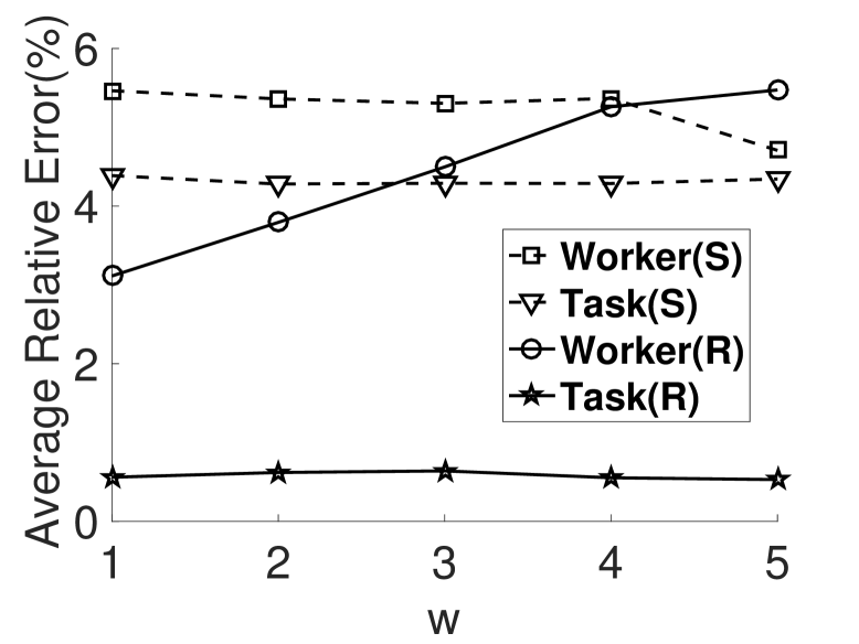
Figure 10: The Prediction Accuracy vs. Window Size $w$.

Comparison with a Straightforward Method. Figure 11 compares the quality score of our MQA approaches (with predicted workers/tasks) with that of the straightforward method which selects assignments in current and next time instances separately (without predictions), where budget $B$ varies from $100$ to $500$. We denote MQA approaches with prediction as GREEDY_WP, D&C_WP, and RANDOM_WP, and those without prediction as GREEDY_WoP, D&C_WoP, and RANDOM_WoP, respectively.

In Figure 11(a), we can see that, the quality scores of MQA with predictions (with solid lines) are higher than that of MQA without prediction (with dash lines), for different budget $B$. This indicates the effectiveness of our MQA approaches over current/predicted workers/tasks, which can achieve better assignment strategy than the ones without prediction (i.e., local optimality). Moreover, either with or without predictions, D&C incurs higher quality scores than GREEDY (since D&C is carefully designed to find assignments with high quality scores via divide-and-conquer), and RANDOM has the lowest score, which implies good quality of our proposed assignment strategies.

Figure 11(b) illustrates the average running time of our GREEDY and D&C approaches, compared with RANDOM, for each time instance. In the figure, due to the prediction and merge costs, D&C_WP requires the highest CPU time to solve the MQA problem, which trades the efficiency for the accuracy. When the budget $B$ increases, the running time of D&C decreases. This is because larger budget $B$ leads to lower cost of selecting assignment pairs under the budget constraint (i.e., lines 12-15 in procedure MQA_D&C of Figure 9). For other approaches, the time cost remains low (i.e., less than 5 seconds) for different $B$ values.

Due to space limitation, we put the results on varying other parameters in Appendix G.

VI-B Performance of the MQA Approaches

The MQA Performance vs. the Range, $[q^{-},q^{+}]$, of Quality Score $q_{ij}$. Figure 12 illustrates the experimental results on different ranges, $[q^{-},q^{+}]$, of quality score $q_{ij}$ from $[0.25,0.5]$ to $[3,4]$ on real data. In Figure 12(a), with the increase of score ranges, quality scores of all the three approaches increase. D&C has higher quality score than GREEDY, which are both higher than RANDOM. From Figure 12(b), RANDOM is the fastest (however, with the lowest quality score), since it randomly selects assignments without considering the quality score maximization. D&C has higher running time than GREEDY (however, higher quality scores than GREEDY). Nonetheless, the running times of GREEDY remain low.

The MQA Performance vs. the Range, $[e^{-},e^{+}]$, of Tasks’ Deadlines $e_{j}$. Figure 13 shows the effect of the range, $[e^{-},e^{+}]$, of tasks’ deadlines $e_{j}$ on the MQA performance over real data, where $[e^{-},e^{+}]$ changes from $[0.25,0.5]$ to $[2,3]$. In Figure 13(a), when the range $[e^{-},e^{+}]$ becomes larger, quality scores of all three approaches also increase. Since a more relaxed (larger) deadline $e_{j}$ of a task $t_{j}$ can be performed by more valid workers, it thus leads to higher quality score (that can be achieved) and processing time (as confirmed by Figure 13(b)). Similar to previous results, D&C can achieve higher quality scores than GREEDY, and both of them outperform RANDOM. Furthermore, GREEDY needs higher time cost than RANDOM, and has lower running time than D&C.

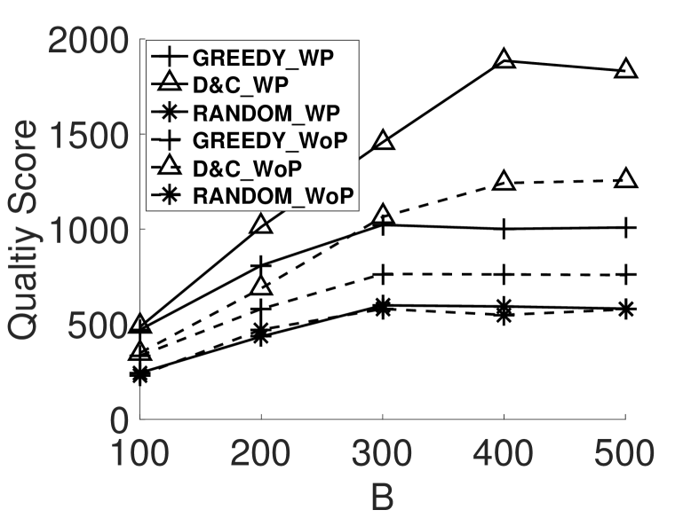
(a) Quality Score

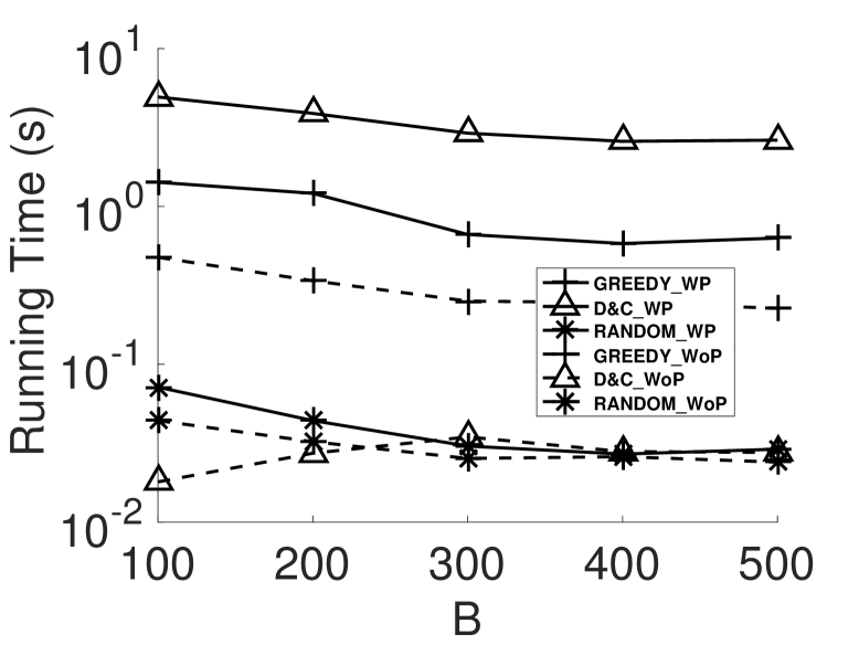
(b) Running Time

Figure 11: Effect of the Budget $B$(Synthetic Data).

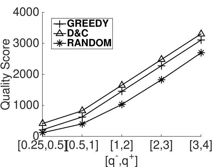
(a) Quality Score

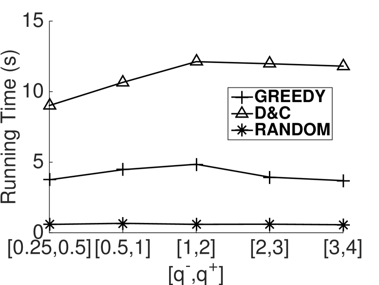
(b) Running Time

Figure 12: Effect of the Range of Quality Score $q_{ij}$ (Real Data).

The MQA Performance vs. the Range, $[v^{-},v^{+}]$, of Workers’ Velocities $v_{i}$. Figure 14 presents the MQA performance with different ranges, $[v^{-},v^{+}]$, of workers’ velocities $v_{i}$ from $[0.1,0.2]$ to $[0.4,0.5]$ on synthetic data, where default values are used for other parameters. In Figure 14(a), when the value range, $[v^{-},v^{+}]$, of velocities of workers increases, the total quality scores of all three approaches decrease. When the range of velocities increases, some worker-and-task pairs with long distances may become valid, which may quickly consume the available budget $B$ and in turn reduce the number of selected pairs. Thus, for larger workers’ velocities, the resulting overall quality score for the selected pairs in GREEDY and D&C approaches decreases. With different velocities, D&C always has higher quality scores than GREEDY, followed by RANDOM. In Figure 14(b), the running times of GREEDY and D&C increase for larger workers’ velocities, since there are more worker-and-task assignments to process. Moreover, RANDOM has the smallest time cost (however, the worst quality score), whereas GREEDY runs faster than D&C, and slower than RANDOM.

The MQA Performance vs. the Number, $m$, of Tasks . Figure 15 varies the total number, $m$, of spatial tasks for $R$ ($=15$ by default) time instance from $1K$ to $10K$ on synthetic data sets, where other parameters are set to their default values. From the experimental results, with the increase of $m$, the total quality scores and time costs of all the three approaches both increase smoothly. This is reasonable, since more tasks lead to more valid pairs, which incur higher quality score for selected assignment pairs, and require higher time cost to process. D&C can achieve higher quality score than GREEDY, which indicates the effectiveness of our proposed D&C approach. Moreover, RANDOM has the worst quality score among the three tested approaches.

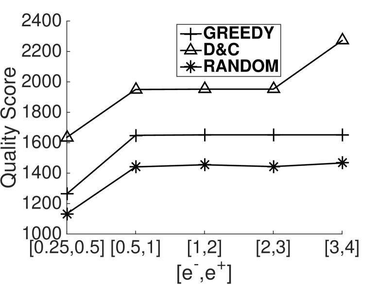
(a) Quality Score

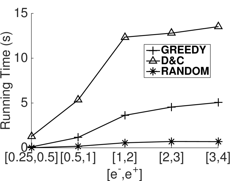
(b) Running Time

Figure 13: Effect of the Range of Tasks’ Deadlines $e_{j}$ (Real Data).

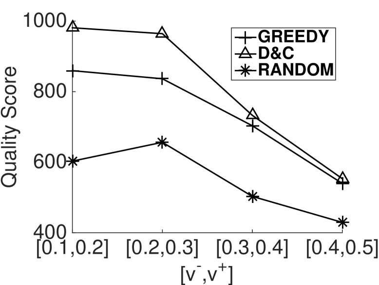
(a) Quality Score

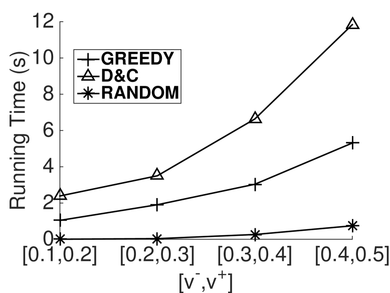
(b) Running Time

Figure 14: Effect of the Range of Velocities $[v^{-},v^{+}]$ (Synthetic Data).

The MQA Performance vs. the Number, $n$, of Workers. Figure 16 examines the effect of the number, $n$, of workers for $R$ ($=15$ by default) time instances on the MQA performance, where $n$ varies from $1K$ to $10K$ and other parameters are set to default values. Similarly, both overall quality scores and running times of three tested approaches increase, for larger $n$ values. Our GREEDY and D&C algorithms can achieve better quality scores than RANDOM. Further, GREEDY has lower time costs than D&C. Nonetheless, the time cost of our approaches smoothly grows with the increasing $n$ values, which indicates good scalability of our MQA approaches.

Due to space limitations, please refer to the experimental results of the effects of the number, $R$, of time instances and the unit price $C$ w.r.t. distance $dist(w_{i},t_{j})$ in Appendix E.

VII related work

There are many previous studies in crowdsourcing systems [6], which usually allow workers to accept task requests and accomplish tasks online. However, these workers do not have to travel to some sites to perform tasks. In contrast, the spatial crowdsourcing system [12, 17] requires workers traveling to locations of spatial tasks, and completes tasks such as taking photos/videos. For instance, some related studies [11, 16] studied the problem of using smart devices (taken by workers) to collect data in real-world applications.

Kazemi and Shahabi [17] classified the spatial crowdsourcing systems from two perspectives: workers’ motivation and publishing models. Regarding the workers’ motivation, there are two types, reward-based and self-incentivised, which inspires workers to do tasks by rewards or volunteering, respectively. Moreover, based on the publishing models, there are two modes, worker selected tasks (WST) [12] and server assigned tasks (SAT) [17, 9, 21, 8], in which tasks are accepted by workers or assigned by workers, respectively. What is more, to handle the requests more quickly, existing studies [23, 24, 22] proposed methods to online process spatial crowdsourcing requests with quality guarantees.

Our MQA problem is reward-based and follows the SAT mode. Prior studies in the SAT mode [17, 9, 21, 8] assigned existing workers to tasks in the spatial crowdsourcing system with distinct goals, for example, maximizing the number of the completed tasks on the server side [17], minimizing the traveling cost for completing a set of given tasks [21], or the reliability-and-diversity score of assignments [9]. In contrast, our MQA problem in this paper has a different goal, that is, maximizing the overall quality score of assignments and under the budget constraint. As a result, we design specific MQA greedy and MQA divide-and-conquer algorithms for our MQA problem, that maximize the quality score (under the budget constraint) rather than other metrics (e.g., the reliability-and-diversity score in [9]), which cannot directly borrow from previous works.

Most importantly, different from the algorithms in existing studies [9, 8] that deal with deterministic workers and tasks, our MQA approaches need to handle predicted workers and tasks, whose locations and other attributes (e.g., distances, quality scores, etc.) are variables (rather than fixed values). Thus, our MQA approaches aims to design the assignment strategy over both current and predicted workers/tasks, which has not been investigated before. Therefore, we cannot directly apply previous techniques (proposed for workers/tasks without prediction) to tackle our MQA problem.

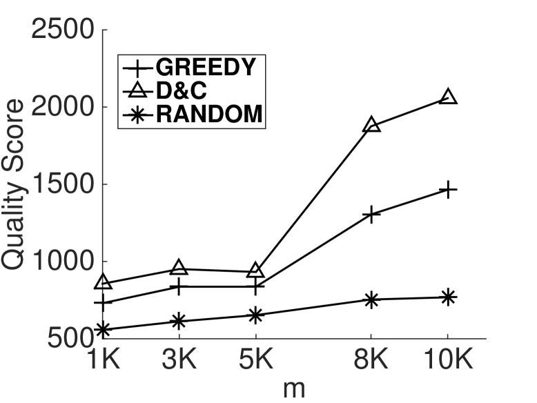
(a) Quality Score

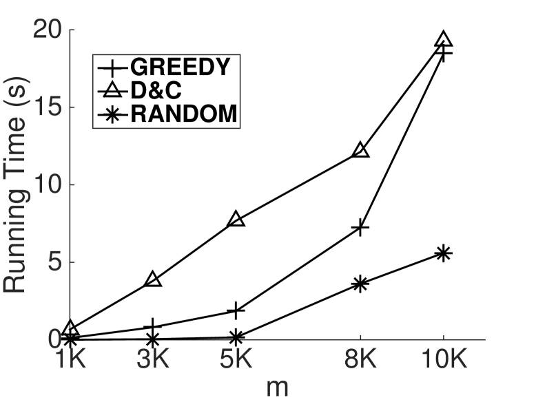
(b) Running Time

Figure 15: Effect of the Number, $m$, of Tasks (Synthetic Data).

VIII conclusion

In this paper, we studied a spatial crowdsourcing problem, named maximum quality task assignment (MQA), which assigns moving workers to spatial tasks satisfying the budget constraint of the traveling cost and achieving a high overall quality score. In order to provide better global assignments, our MQA approaches are based on the assignment selection strategy over both current and (predicted) future workers/tasks. We propose an accurate prediction approach to estimate both quality/location distributions of workers/tasks. We prove that the MQA problem is NP-hard, and thus intractable. Alternatively, we propose efficient heuristics, including MQA greedy and MQA divide-and-conquer approaches, to obtain better global assignments. Extensive experiments have been conducted to confirm the efficiency and effectiveness of our proposed MQA processing approaches.

IX Acknowledgment

Peng Cheng and Lei Chen are supported in part by Hong Kong RGC Project N HKUST637/13, NSFC Grant No. 61328202, NSFC Guang Dong Grant No. U1301253, National Grand Fundamental Research 973 Program of China under Grant 2014CB340303, HKUST-SSTSP FP305, Microsoft Research Asia Gift Grant, Google Faculty Award 2013 and ITS170. Xiang Lian is supported by Lian Start Up No. 220981. Cyrus Shahabi’s work has been funded in part by NSF grants IIS-1320149 and CNS-1461963.

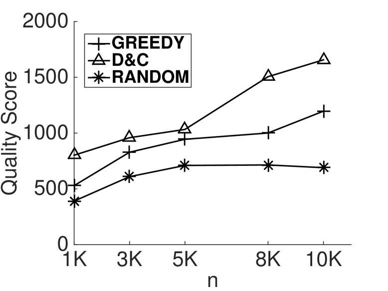
(a) Quality Score

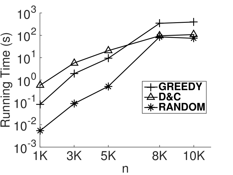
(b) Running Time

Figure 16: Effect of the Number, $n$, of Workers (Synthetic Data).

-A Proof of Lemma 2.1

Proof:

We prove the lemma by a reduction from the 0-1 knapsack problem. A 0-1 knapsack problem can be described as follows: Given a set, $C$, of $n$ items $a_{i}$ numbered from 1 up to $n$, each with a weight $w_{i}$ and a value $v_{i}$, along with a maximum weight capacity $W$, the 0-1 knapsack problem is to find a subset $C^{\prime}$ of $C$ that maximizes $\sum_{a_{i}\in C^{\prime}}v_{i}$ subjected to $\sum_{a_{i}\in C^{\prime}}w_{i}\leq W$.

For a given 0-1 knapsack problem, we can transform it to an instance of MQA as follows: at timestamp $p$, we give $n$ pairs of worker and task, such that for each pair of worker and task $\langle w_{i},t_{i}\rangle$, the traveling cost $c_{ii}=w_{i}$ and the quality score $q_{ii}=v_{i}$. Also, we set the global budget $B=W$. At the same time, for any pair of worker and task $\langle w_{i},t_{j}\rangle$ where $t_{j}\neq t_{i}$, we make $c_{ij}\gg c_{ii}$ and $q_{ij}\leq q_{ii}$. Thus, in the assignment result, it is only possible to select worker-and-task pairs with same subscripts. Then, for this MQA instance, we want to achieve an assignment instance set $I_{p}$ of some pairs of worker and task with same subscripts that maximizes the quality score $\sum_{\forall\langle w_{i},t_{i}\rangle\in I_{p}}q_{ii}$ subjected to $\sum_{\forall\langle w_{i},t_{i}\rangle\in I_{p}}c_{ii}\leq B$.

Given this mapping, we can show that the 0-1 knapsack problem instance can be solved, if and only if the transformed MQA problem can be solved.

This way, we can reduce 0-1 knapsack problem to the MQA problem. Since 0-1 knapsack problem is known to be NP-hard [25], MQA is also NP-hard, which completes our proof. ∎

-B The Pseudo Code of the Grid-based Prediction Algorithm

Figure 17 shows the pseudo code of our grid-based prediction algorithm, namely MQA_Prediction, which predicts the number of workers/tasks in each cell, $cell_{i}$, of the grid index by using the linear regression (lines 3-4), and generates worker/task samples with the estimated sizes (lines 5-6).

Procedure MQA_Prediction { Input: worker sets $\mathbb{W}=\{W_{p-w+1},...,W_{p}\}$ and task sets $\mathbb{T}=\{T_{p-w+1},$ $...,$ $T_{p}\}$ at the latest $w$ time instances, and a grid index $\mathcal{I}$ Output: future workers and tasks in $W_{p+1}$ and $T_{p+1}$, respectively, for the next time instance at timestamp $(p+1)$ (1) let $W_{p+1}=\emptyset$ and $T_{p+1}=\emptyset$ (2) for each cell $cell_{i}$ in $\mathcal{I}$ (3) estimate the future number, $|W_{p+1}^{(i)}|$, of workers in $cell_{i}$ by the linear regression (4) estimate the future number, $|T_{p+1}^{(i)}|$, of tasks in $cell_{i}$ by the linear regression (5) randomly generate $|W_{p+1}^{(i)}|$ worker samples for $cell_{i}$, and add them to $W_{p+1}$ (6) randomly generate $|T_{p+1}^{(i)}|$ task samples for $cell_{i}$, and add them to $T_{p+1}$ (7) return $W_{p+1}$ and $T_{p+1}$ }

Figure 17: The Grid-Based Worker/Task Prediction Algorithm.

-C Cost-Model-Based Estimation of the Best Number of the Decomposed Subproblems

The Cost, $F_{D}$, of Decomposing Subproblems. From Algorithm MQA_Decomposition (in Figure 7), we first need to retrieve all valid worker-and-task assignment pairs (line 3), whose cost is $O(m^{\prime}\cdot n^{\prime})$, where $m^{\prime}$ and $n^{\prime}$ are the numbers of both current/future tasks and workers, respectively. Then, we will divide each problem into $g$ subproblems, whose cost is given by $O(m^{\prime}\cdot g+m^{\prime})$ on each level. For level $k$, we have $m^{\prime}/g^{k}$ tasks in each subproblem $M^{(k)}_{i}$. We will further partition it into $g$ more subproblems, $M^{(k+1)}_{j}$, recursively, and each one will have $m^{\prime}/g^{k+1}$ tasks. In order to obtain $m^{\prime}/g^{k+1}$ tasks in each subproblem $M^{(k+1)}_{j}$, we first need to find the anchor task, which needs $O(m^{\prime}/g^{k})$ cost, and then retrieve the rest tasks, which needs $O(m/g^{k+1})$ cost. Moreover, since we have $g^{k+1}$ subproblems on level $(k+1)$, the cost of decomposing tasks on level $k$ is given by $O(m^{\prime}\cdot g+m^{\prime})$.

Since there are totally $log_{g}(m^{\prime})$ levels, the total cost of decomposing the MQA problem is given by:

$$F_{D}=m^{\prime}\cdot n+(m^{\prime}\cdot g+m^{\prime})\cdot log_{g}(m^{\prime}).$$

Figure 18: Effect of Distributions of Workers and Tasks on Quality Score (Synthetic Data).

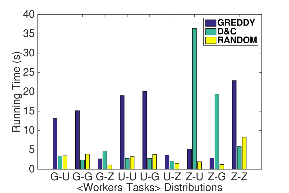
Figure 19: Effect of Distributions of Workers and Tasks on Running Time (Synthetic Data).

The Cost, $F_{C}$, of Recursively Conquering Subproblems.

Let function $F_{C}(x)$ be the total cost of recursively conquering a subproblem, which contains $x$ spatial tasks. Then, we have the following recursive function:

$$F_{C}(m^{\prime})=g\cdot F_{C}(\left\lceil\frac{m^{\prime}}{g}\right\rceil).$$

Assume that $deg_{t}$ is the average number of tasks in the assignment instance set $I_{p}$. Then, the base case of function $F_{C}(x)$ is the case that $x=1$, in which we greedily select one worker-and-task pair from $deg_{t}$ pairs to achieve the highest quality score (via the greedy algorithm). Thus, we have $F_{C}(1)=2deg_{t}^{2}$.

From the recursive function $F_{C}(x)$ and its base case, we can obtain the total cost of the recursive invocation on levels from 1 to $log_{g}(m)$ below:

$$\sum_{k=1}^{\log_{g}(m^{\prime})}F_{c}(m^{\prime}/g^{k})=\frac{2(m^{\prime}-1)deg_{t}^{2}}{g-1}.$$

The Cost, $F_{M}$, of Merging Subproblems. Next, we provide the cost, $F_{M}$, of merging subproblems by resolving conflicts. For level $k$, we have $g^{k}$ subproblems and $m^{\prime}/g^{k}$ tasks in each subproblem $M^{(k)}_{i}$. When merging the result of one subproblem $M^{(k)}_{i}$ to the current maintained assignment instance set $I_{p}$, there are at most $m^{\prime}/g^{k}$ conflicted workers as each task is only assigned with one worker. In addition, for level $k$, we need to merge the results of $(g^{k}-1)$ subproblems to the current maintained assignment instance set. Moreover, when resolving conflict of one worker, we may need to greedily pick one available worker from $deg_{t}$ workers, which costs $2deg_{t}^{2}$.

Therefore, the worst-case cost of resolving conflicts during resolving conflicts of workers can be given by:

$$F_{M}=\sum_{k=1}^{\log_{g}(m^{\prime})}2deg_{t}^{2}(g^{k}-1)\frac{m}{g^{k}}=2deg_{t}^{2}(\frac{m\log m}{\log g}-\frac{g(m-1)}{g-1}).$$

The Cost, $F_{B}$, of the Budget Adjustment on Subproblems. Then, we provide the cost, $F_{B}$, of the budget adjustment in line 15 of the D&C algorithm (in Figure 9), or lines 17-28 in procedure MQA_Budget_Constrained_Selection (Figure 8). Since each task is assigned with at most one worker, the number of candidate pairs is at most same as the number of tasks. For a subproblem with $m^{\prime}/g^{k}$ tasks on level $k$, lines 20-25 of Figure 8 need at most $(m^{\prime}/g^{k})^{2}$ cost. In addition, line 26 needs $|S_{p}|$ cost, which is also at most $(m^{\prime}/g^{k})^{2}$ cost. There are at most $(m^{\prime}/g^{k})$ iterations, each of which selects at least one pair.

Therefore, the cost of the budget adjustment while merging subproblems can be given by:

$$F_{B}=\sum_{k=0}^{\log_{g}(m^{\prime})}g^{k}\cdot 2(\frac{m^{\prime}}{g^{k}})^{3}=\sum_{k=0}^{\log_{g}(m^{\prime})}\frac{2m^{\prime 2}}{g^{2k}}=\frac{2g^{2}(m^{\prime 2}-1)}{g^{2}-1}.$$ (11)

The Total Cost of the $g$-D&C Approach. The total cost, $cost_{D\&C}$, of the D&C algorithm can be given by summing up four costs, $F_{D}$, $F_{C}$, $F_{M}$, and $F_{B}$. That is, we have:

$$cost_{D\&C} = F_{D}+\sum_{k=1}^{log_{g}(m^{\prime})}F_{c}(m^{\prime}/g^{k})+F_{M}+F_{B}.$$ (12)

We take the derivation of $cost_{D\&C}$ (given in Eq. (12)) over $g$, and let it be 0. In particular, we have:

$$\frac{\partial cost_{D\&C}}{\partial g} = \frac{m^{\prime}\log m^{\prime}(g\log g-g-1-2deg_{t}^{2})}{g\log^{2}(g)}$$ (13)

$$-\frac{4g(m^{\prime 2}-1)}{(g^{2}-1)^{2}}=0.$$

We notice that when $g=2$, $\frac{\partial cost_{D\&C}}{\partial g}$ is much smaller than 0 but increases quickly when $g$ grows. In addition, $g$ can only be an integer. Then we can try the integers like 2, 3, and so on, until $\frac{\partial cost_{D\&C}}{\partial g}$ is above 0.

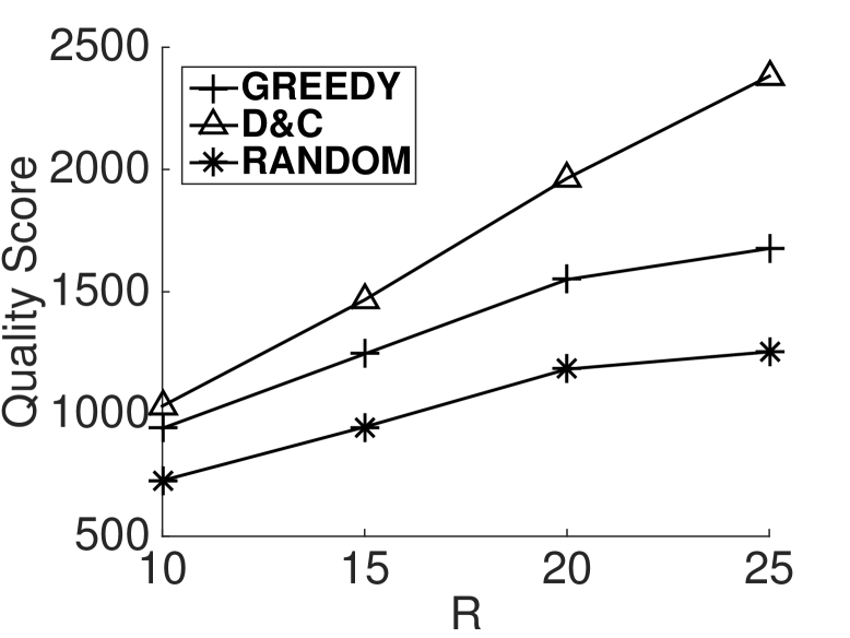
(a) Quality Score

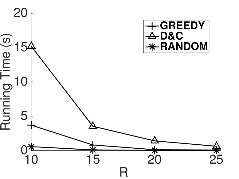
(b) Running Time

Figure 20: Effect of the Number, $R$, of Time Instances (Synthetic Data).

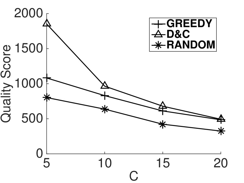
(a) Quality Score

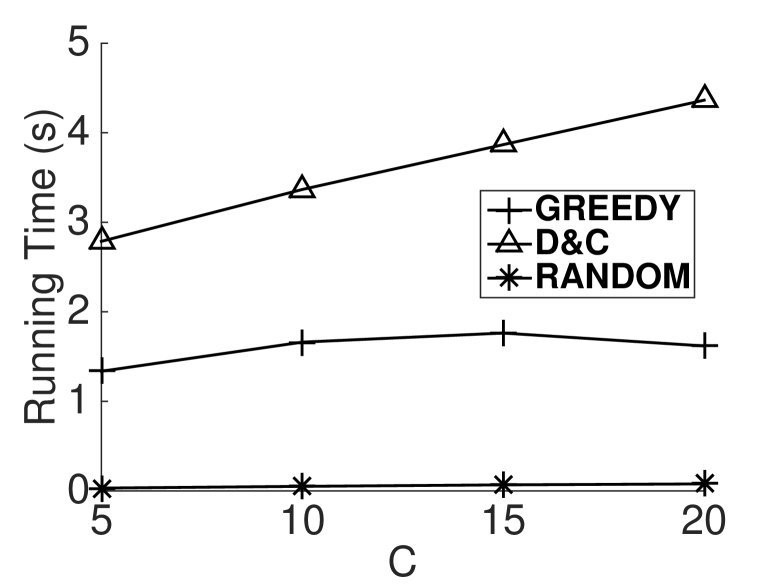
(b) Running Time

Figure 21: Effect of the Unit Price $C$ w.r.t. Distance $dist(w_{i},t_{j})$ (Synthetic Data).

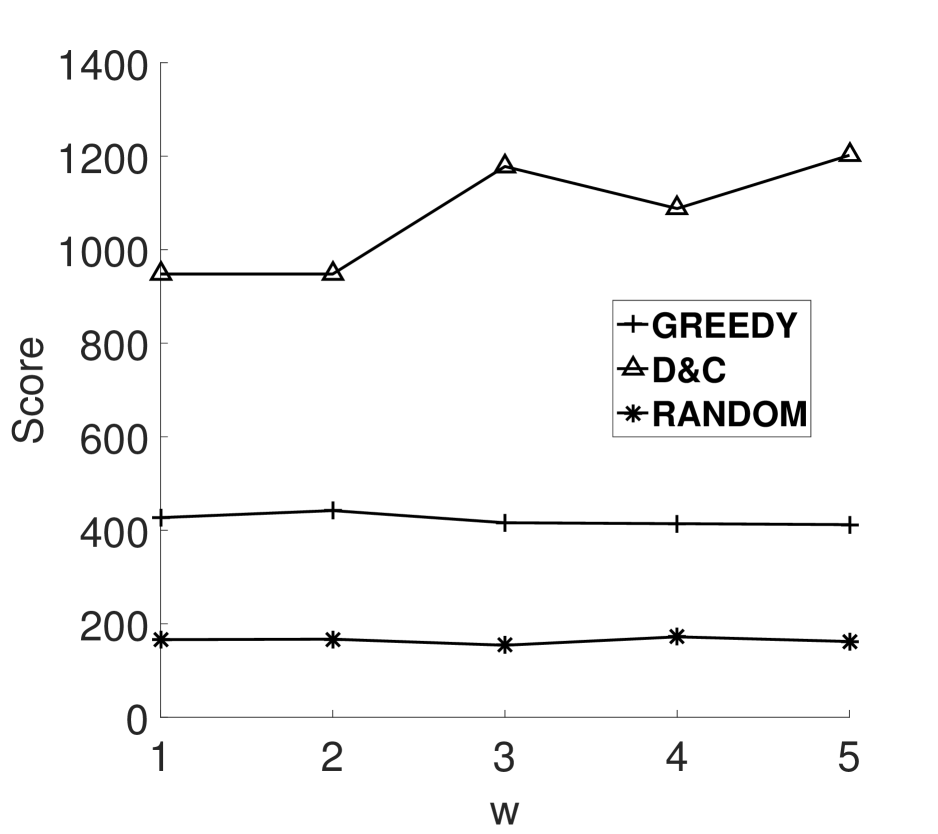
(a) Quality Score (GAUS)

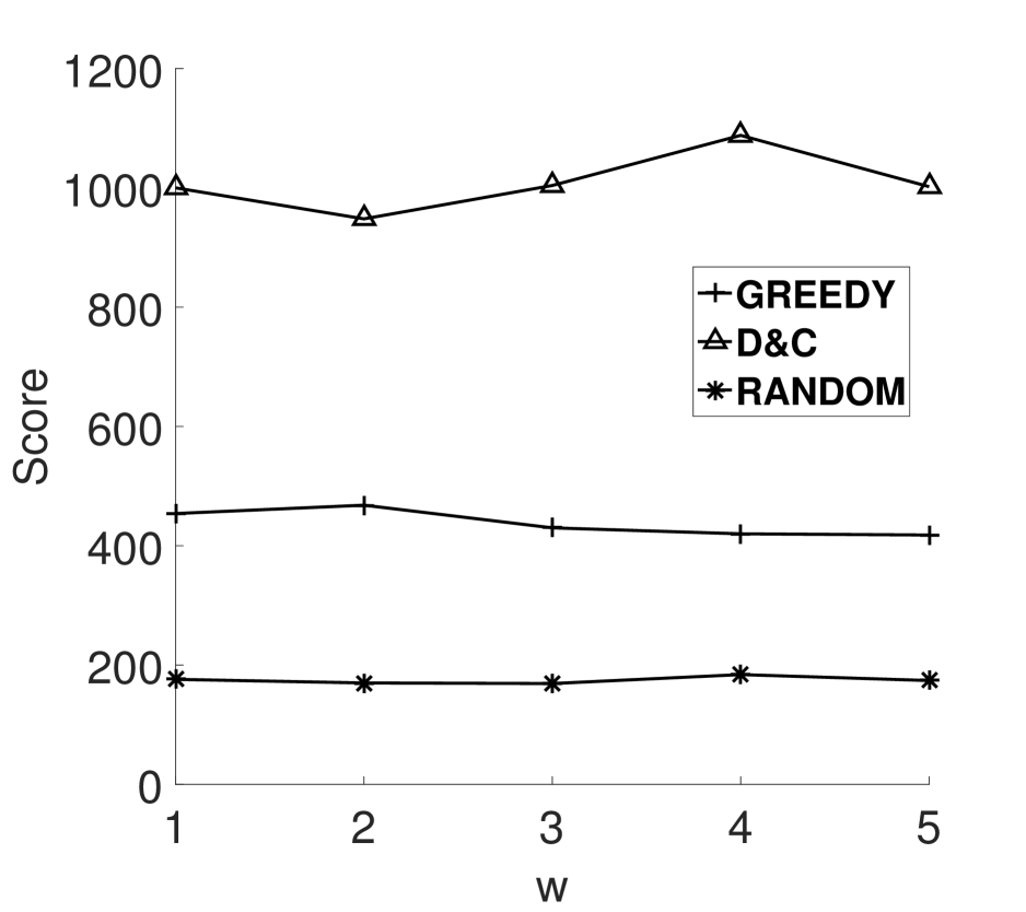
(b) Quality Score (UNIF)

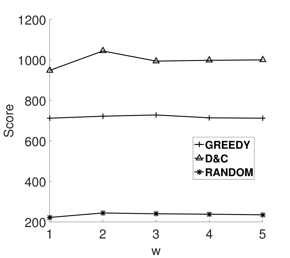
(c) Quality Score (ZIPF)

Figure 22: Effect of the Window Size $w$ (Synthetic Data).

-D Results with Different Worker-Task Distributions

In this section, we present the experimental results for workers and tasks with different location distributions, where parameters of synthetic data are set to default values. We denote the Uniform distribution as U, the Gaussian distribution as G, and the Zipf distribution as Z. Then, for $\langle worker$$-$$task\rangle$ distributions, we tested the quality score and running time over 9 distribution combinations, including G-U, G-G, G-Z, U-U, U-G, U-Z, Z-U, Z-G, and Z-Z, and the results are shown in Figures 18 and 19.

Similar to previous results, as shown in Figure 18, the D&C algorithm can achieve the highest quality score, compared with GREEDY and RANDOM, over all the 9 worker/task distribution combinations. For the running time, as illustrated in Figure 19, with different combinations of worker/task distributions, D&C can achieve low time cost in most cases. Only for Z-U and Z-G, D&C incurs higher time cost than GREEDY and RANDOM, due to the unbalanced distributions of workers and tasks. In particular, GREEDY and RANDOM iteratively assign one valid pair and maintain the rest of valid pairs in each iteration. When the distributions of workers and tasks are similar, for example, G-G, U-U, and Z-Z, running times of GREEDY and RANDOM become longer than D&C. Especially, for Z-Z, almost all the workers can reach all the tasks, which leads to the highest number of valid pairs among all the 9 distribution combinations. As a result, both GREEDY and RANDOM need much higher running time than that of other distribution combinations. In general, with different worker and task distributions, our GREEDY and D&C can both achieve high quality scores (with small time cost).

-E The MQA Performance vs. the Number, $R$, of Time Instances and the Unit Price $C$ w.r.t. Distance $dist(w_{i},t_{j})$

The MQA Performance vs. the Number, $R$, of Time Instance. Figure 20 reports the experimental results for different numbers, $R$, of time instance from 10 to 25 on synthetic data sets, where other parameters are set to default values. In Figure 20(a), when the number, $R$, of time instances increases, the total quality score of three MQA approaches also increases. Since we consider a fixed time interval $P$ with more time instances (each with budget $B$), the total quality score within interval $P$ expects to increase for more time instances. D&C can achieve higher quality scores than GREEDY.

In Figure 20(b), when $R$ becomes larger, the running time of all the three tested approaches decreases. This is because, given $m$ tasks and $n$ workers within time interval $P$, for more time instances, the average number of workers/tasks per time instance decreases, which leads to lower time cost per time instance. Similar to previous results, the running time of GREEDY is lower than that of D&C.

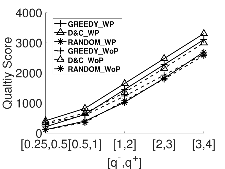
(a) Quality Score

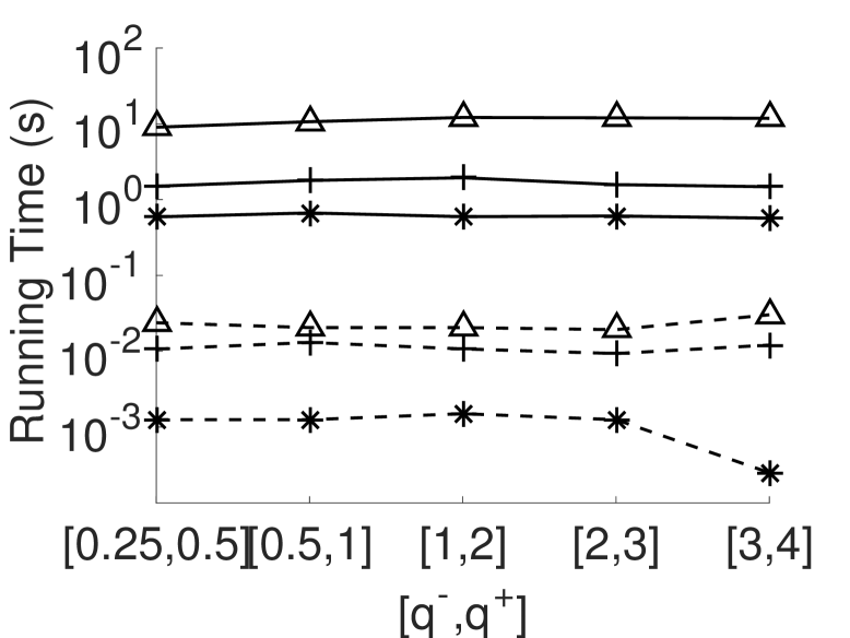
(b) Running Time

Figure 23: Effect of the Range of Quality Score $q_{ij}$ (Real Data).

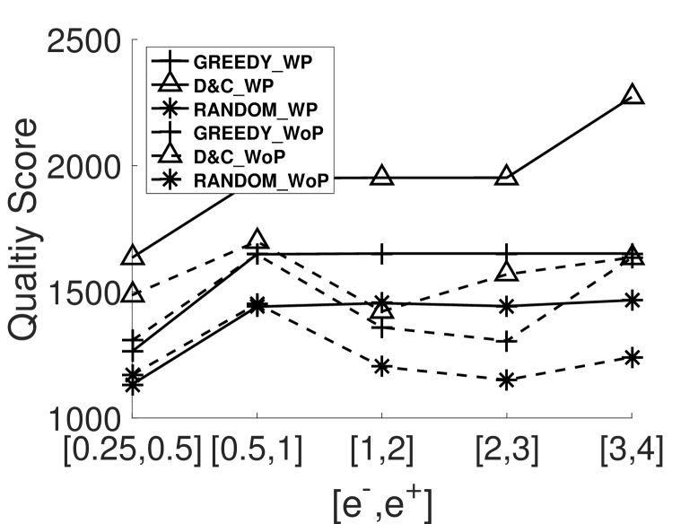
(a) Quality Score

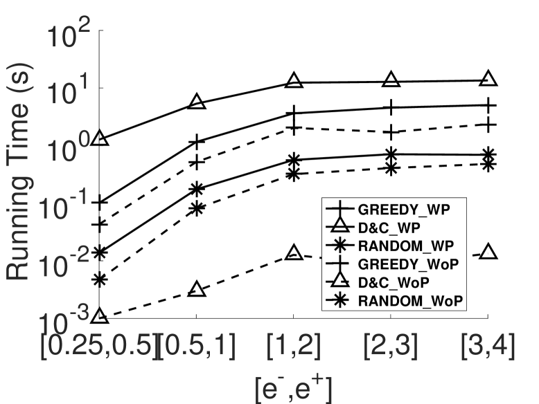
(b) Running Time

Figure 24: Effect of the Range of Tasks’ Deadlines $e_{j}$ (Real Data).

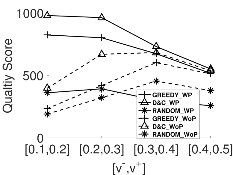
(a) Quality Score

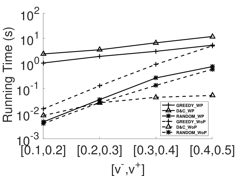
(b) Running Time

Figure 25: Effect of the Range of Velocities $[v^{-},v^{+}]$ (Synthetic Data).

The MQA Performance vs. the Unit Price $C$ w.r.t. Distance $dist(w_{i},t_{j})$. Figure 21 illustrates the experimental results on different unit prices $C$ w.r.t. distance $dist(w_{i},t_{j})$ from $5$ to $20$ over synthetic data, where other parameters are set to default values. In Figure 21(a), when the unit price $C$ increases, the overall quality scores of all the three approaches decrease. This is because for larger $C$, the number of valid worker-and-task pairs for each time instance decreases, under the budget constraint. Thus, the overall quality score of all the selected assignments also expects to decrease for large $C$. Similar to previous results, D&C has higher quality scores than GREEDY. In Figure 21(b), running times of GREEDY and RANDOM are not very sensitive to $C$. However, with large $C$, the running time of D&C increases, since we need to check the constraint of budget from lower divide-and-conquer levels, which increases the total running time. For different $C$ values, GREEDY has lower running times than D&C.

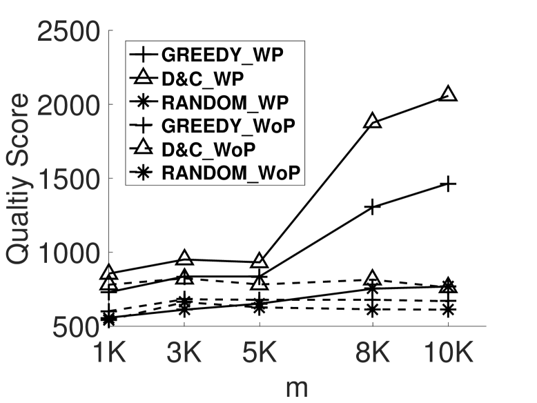
(a) Quality Score

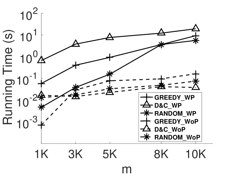
(b) Running Time

Figure 26: Effect of the Number, $m$, of Tasks (Synthetic Data).

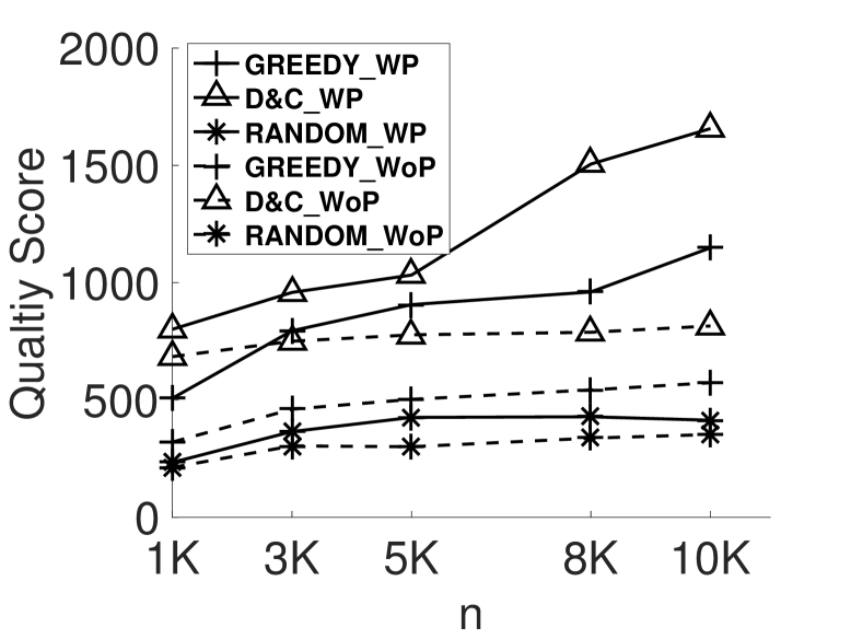
(a) Quality Score

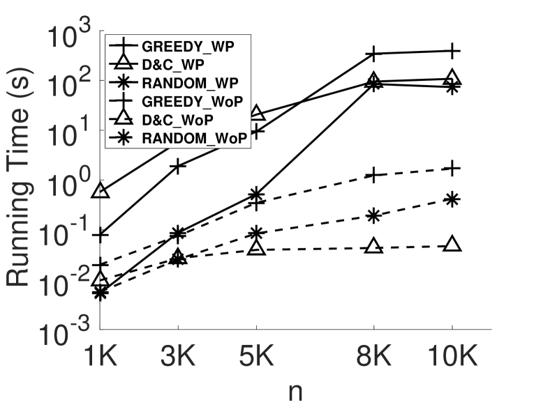
(b) Running Time

Figure 27: Effect of the Number, $n$, of Workers (Synthetic Data).

-F The MQA Performance vs. the Window Size $w$

We show the results of quality scores by varying window size on different workers distributions in Figure 22. We can see the sliding window size affects the quality score slightly for GREEDY and RANDOM. For D&C, it can achieve the highest quality score when the window size equals to 3 on workers with Gaussian Distribution (as shown in Figure 22(a)), and equals to 4 and 2 on workers with Uniform and Zipf distribution respectively.

-G Results of Comparison with Straightforward Methods

Figure 23 to Figure 27 compare the quality scores and running times of our MQA approaches (with predicted workers/tasks) with that of the straightforward method which selects assignments at current and next time instances separately (without predictions) by varying the range [$q^{−}$, $q^{+}$] of quality score $q_{ij}$, the range [$e^{-}$, $e^{+}$] of tasks’ deadlines $e_{j}$, the range [$v^{-}$, $v^{+}$] of workers’ velocities $v_{i}$, the number of tasks $m$ and the number of workers $n$. We denote MQA approaches with prediction as GREEDY_WP, D&C_WP, and RANDOM_WP, and those without prediction as GREEDY_WoP, D&C_WoP, and RANDOM_WoP, respectively.

References

- [1] Gigwalk. http://www.gigwalk.com.
- [2] Google street view. https://www.google.com/maps/views/streetview.
- [3] Taskrabbit. https://www.taskrabbit.com.
- [4] Waze. https://www.waze.com.
- [5] S. Borzsony, D. Kossmann, and K. Stocker. The skyline operator. In ICDE, 2001.
- [6] M. F. Bulut, Y. S. Yilmaz, and M. Demirbas. Crowdsourcing location-based queries. In PERCOM Workshops, 2011.
- [7] Z. Chen, R. Fu, Z. Zhao, Z. Liu, L. Xia, L. Chen, P. Cheng, and et al. gmission: A general spatial crowdsourcing platform. VLDB, 2014.
- [8] P. Cheng, X. Lian, L. Chen, J. Han, and J. Zhao. Task assignment on multi-skill oriented spatial crowdsourcing. TKDE, 2016.
- [9] P. Cheng, X. Lian, Z. Chen, and et al. Reliable diversity-based spatial crowdsourcing by moving workers. VLDB.
- [10] E. Cho, S. A. Myers, and J. Leskovec. Friendship and mobility: user movement in location-based social networks. In SIGKDD, 2011.
- [11] C. Cornelius, A. Kapadia, D. Kotz, D. Peebles, and et al. Anonysense: privacy-aware people-centric sensing. In MobiSys, 2008.
- [12] D. Deng, C. Shahabi, and U. Demiryurek. Maximizing the number of worker’s self-selected tasks in spatial crowdsourcing. In SIGSPATIAL GIS, 2013.
- [13] C. M. Grinstead and J. L. Snell. Introduction to probability. American Mathematical Soc., 2012.
- [14] B. E. Hansen. Lecture notes on nonparametrics. Lecture notes, 2009.
- [15] G. Jovanovic-Dolecek. Demo program for central limit theorem. In MWSCAS, volume 1, 1997.
- [16] S. S. Kanhere. Participatory sensing: Crowdsourcing data from mobile smartphones in urban spaces. In MDM, volume 2, 2011.
- [17] L. Kazemi and C. Shahabi. Geocrowd: enabling query answering with spatial crowdsourcing. In SIGSPATIAL GIS, 2012.
- [18] S. H. Kim, Y. Lu, G. Constantinou, C. Shahabi, G. Wang, and R. Zimmermann. Mediaq: mobile multimedia management system. In MMSys, 2014.
- [19] C. L. Lawson and R. J. Hanson. Solving least squares problems. volume 161. SIAM, 1974.
- [20] J. J. Levandoski, M. Sarwat, A. Eldawy, and M. F. Mokbel. Lars: A location-aware recommender system. In ICDE, 2012.
- [21] Q. Liu, T. Abdessalem, H. Wu, Z. Yuan, and S. Bressan. Cost minimization and social fairness for spatial crowdsourcing tasks. In DASFAA, 2016.
- [22] S. Tianshu, T. Yongxin, W. Libin, S. Jieying, and et al. Trichromatic online matching in real-time spatial crowdsourcing. ICDE, 2017.
- [23] Y. Tong, J. She, B. Ding, L. Chen, and et al. Online minimum matching in real-time spatial data: experiments and analysis. VLDB, 2016.
- [24] Y. Tong, J. She, B. Ding, L. Wang, and L. Chen. Online mobile micro-task allocation in spatial crowdsourcing. ICDE, 2016.
- [25] V. V. Vazirani. Approximation algorithms. Springer Science & Business Media, 2013.