Surface transport in plasma-balls

Abstract

We study the surface transport properties of stationary localized configurations of relativistic fluids to the first two non-trivial orders in a derivative expansion. By demanding that these finite lumps of relativistic fluid are described by a thermal partition function with arbitrary stationary background metric and gauge fields, we are able to find several constraints among surface transport coefficients. At leading order, besides recovering the surface thermodynamics, we obtain a generalization of the Young-Laplace equation for relativistic fluid surfaces, by considering a temperature dependence in the surface tension, which is further generalized in the context of superfluids. At the next order, for uncharged fluids in 3+1 dimensions, we show that besides the 3 independent bulk transport coefficients previously known, a generic localized configuration is characterized by 3 additional surface transport coefficients, one of which may be identified with the surface modulus of rigidity. Finally, as an application, we study the effect of temperature dependence of surface tension on some explicit examples of localized fluid configurations, which are dual to certain non-trivial black hole solutions via the AdS/CFT correspondence.

1 Introduction

The theory of hydrodynamics provides us with a tractable effective framework to study the low-energy near-equilibrium states in any finite temperature system with a well behaved microscopic description. Although the description of these states in terms of the microscopic degrees of freedom may be very complicated, hydrodynamics allows us to describe them with a few effective degrees of freedom - the fluid fields. This effective theory is constructed purely on the basis of symmetries inherent to the microscopic theory, in addition to certain empirical assumptions like the second law of thermodynamics (see Landau:1987gn ). The information of the underlying field theory is encoded, in a phenomenological way, in the transport coefficients that characterize the effective macroscopic description.

Although hydrodynamics is a very old and well studied subject, recently there has been a renewed interest in it, particularly after the discovery of its connections with black hole dynamics in the context of the AdS/CFT correspondence Bhattacharyya:2008jc . These recent studies have valuably contributed to the improved understanding of the structural features of the subject and has led to the unraveling of new transport phenomenon Banerjee:2008th ; Erdmenger:2008rm ; Son:2009tf ; Bhattacharya:2011eea ; Herzog:2011ec ; Bhattacharya:2011tra . Most of these latest developments mainly focus on the description of states in which the same phase of the fluid fills the entire spacetime, which is taken to be a non-compact pseudo-Riemanian manifold. In other words, the hydrodynamics that has been explored in most of these recent developments is the effective theory of a class of states, which does not involve any fluid surface or a phase boundary.

In this paper we proceed to analyze the situation where the class of states described by the effective theory of hydrodynamics is extended to incorporate the states that include a fluid surface, which separates two phases. We will mainly focus on finite lumps of relativistic fluids, which occupies only a finite subspace of an otherwise non-compact spacetime. One of the concrete examples of our set up is described in Aharony:2005bm , where metastable finite lumps of the deconfined phase of $\mathcal{N}=4$ SYM is separated from the confined phase by a phase boundary. In the large $N$ limit, such a situation can be described by a metastable fireball of plasma-fluid separated from the vacuum by a fluid surface. Although we have a set up similar to Aharony:2005bm at the back of our mind, we wish to clarify that in this paper we have taken a purely field theory perspective and we make no use of the AdS/CFT correspondence in any way.

We would like to highlight the fact that the behaviour of the microscopic field theory, at or near the surface, can in general be quite different from that in the bulk. This difference would be captured by new surface transport coefficients in the effective theory. Some of these new surface transport coefficients would simply encode the way in which the bulk transport coefficients are modified at the surface, while others would represent entirely new transport properties, particular to the existence of the fluid surface.

A very well known example of such a surface phenomenon, at the leading order in derivative expansion, is surface tension. In this paper, we study the surface transport coefficients, at the subleading order, and investigate the relations that may exists between them and the bulk transport coefficients. We would like to emphasize, that the surface transport coefficients carry entirely new information about the microscopics and modify the fluid equations at the surface very non-trivially. For instance, knowledge of the equation of state for a fluid, tells us nothing about how the surface tension depends on temperature.

The study of surface transport has been carried out to some extent in the context of fluids which are confined to a thin submanifold of spacetime Armas:2013hsa ; Armas:2013goa ; Armas:2014rva . This is the case in which the bulk fluid is not present or, alternatively, its pressure and higher-order transport coefficients vanish at the surface. In such situations, a systematic analysis based on an effective action approach Armas:2013hsa , underlying symmetries and positivity of the entropy current Armas:2013goa ; Armas:2014rva have been used to constrain the form of the equations of motion up to second order in derivatives. One of the particular features inherent to the study of dynamical surfaces is that, due to possible deformations along directions transverse to it, new transport coefficients appear encoding the response of the surface to bending. One such transport coefficient is the surface modulus of rigidity Armas:2013hsa . The novelty in this paper resides on the fact that the system we study is a more intricate one, in which both the fluid residing in the bulk and the fluid living on the surface constitute the same system.

One of the central simplifying assumptions that we shall make in this paper is that we will only consider stationary fluid configuration. For the case of stationary space-filling relativistic fluids without any surface, the constitutive relations and hence the equations of motion could be significantly constrained from a simple physical criterion. This criterion is that we demand the symmetry currents, including the stress tensor, to follow from an equilibrium partition function Banerjee:2012iz ; Jensen:2012jh ; Jain:2012rh ; Banerjee:2012cr ; Bhattacharyya:2012xi .

The stationary fluid configurations are considered in the presence of non-trivial background fields, like the metric and the gauge fields corresponding to other conserved charges. These background fields are considered to be slowly varying, with respect to the length scale associated with the radius of time-circle, in this finite temperature description. These slowly varying background fields serve as sources in the relativistic fluid equations. On solving these equations, the fluid variables are expressed in terms of these background sources. Now, if we substitute this solution of the fluid variables, back into a putative action for stationary configurations, we obtain the equilibrium partition function expressed as a functional of background fields. Since, the fluid equations, and hence the solutions of fluids fields, are constructed in a derivative expansion, therefore the partition function could be expanded in a derivative expansion, in terms of these background fields and their derivatives.

There are several advantages in considering the partition function expressed in terms of the background fields, (instead of the fluid variables) as the starting point of the analysis. This description is unaffected by any ambiguities related to choice of frames, as we move to higher order in derivatives. Also, while constructing the derivative expansions for the partition function, there is no need to account for constrains arising from lower order equation of motion, as is required while writing down the constitutive relations.

It is straightforward to compute the symmetry currents from the partition function by varying it with respect to the background fields. Then, we proceed to compare the symmetry currents so obtained, with that which is expressed in terms of the fluid variables through the constitutive relations. This comparison not only yields the expressions for the fluid variables in terms of the background fields, specific to the stationary configurations under consideration, but also provides non-trivial relations between the transport coefficients (see §1.1 for more details). Although derived by analyzing stationary fluid configurations, these relations between transport coefficients are expected to hold even away from equilibrium. In this paper, one of our principal goals would be to adopt a such a method to constrain transport properties at the surface of relativistic fluids.

1.1 The general set up

1.1.1 Generalities of the partition function analysis

Consider a relativistic fluid living in a spacetime $\mathcal{N}$, equipped with a time-like Killing vector, which has the most general stationary metric

$$ds^{2}\equiv\mathcal{G}_{\mu\nu}dx^{\mu}dx^{\nu}=-e^{-2\sigma(x)}\left(dt+a_{i}(x)dx^{i}\right)^{2}+g_{ij}(x)dx^{i}dx^{j}~{}~{}.$$ (1)

Here, the metric functions, depends only on the spatial coordinates $x$, and $\partial_{t}$ is our time-like Killing vector. Here $g_{ij}$ is the metric on spatial manifold obtained by reducing on the time-circle , which we shall denote by $\mathcal{N}_{s}$.

In some of our discussions, we will also include a conserved global $U(1)$. The background gauge fields for this $U(1)$ take the form

$$\mathcal{A}=\mathcal{A}_{0}(x)dx^{0}+\mathcal{A}_{i}(x)dx^{i}~{}~{}.$$ (2)

Since none of the functions depend on time, all the quantities of interest, including the conserved currents, can be dimensionally reduced on the time-circle, whose radius we take to be $T_{0}$. It is possible to restrict to this reduced language, focusing only on $\mathcal{N}_{s}$, for most of the discussions relating to the partition function.

Among the reduced quantities, time-translation invariance survives as a gauge invariance corresponding to the Kaluza-Klein gauge field $a_{i}(x)$. All our constructions starting from the partition function, must be manifestly invariant under this Kaluza-Klein gauge transformation.

Since the $U(1)$ gauge fields in (2) transform non-trivially under the Kaluza-Klein gauge transformation, it is convenient to define a new set of shifted gauge fields which are manifestly invariant under it

$$A_{i}=\mathcal{A}_{i}-\mathcal{A}_{0}a_{i},~{}~{}A_{0}=\mathcal{A}_{0}~{}~{}.$$ (3)

Thus $\mathcal{B}\equiv\{\sigma(x),a_{i}(x),g_{ij}(x),A_{0}(x),A_{i}(x),T_{0}\}$ constitutes the set of background data in terms of which the partition function is to be expressed.

Now, since we wish to describe a finite lump of relativistic fluid, we will assume that the fluid is confined to a sub-manifold of $\mathcal{N}$ of the same dimensionality as the spacetime, which we shall denote by $\mathcal{M}$. The fluid surface is considered to be a co-dimension one hypersurface. We shall denote the fluid surface by $f(x)=0$, where $f(x)$ is taken to be independent of time, following our stationary assumption. In fact, $f(x)$ can be taken to be a spatial coordinate itself, which is positive inside the fluid and negative outside. The region inside, $f(x)=0$ is $\mathcal{M}$, which can again be reduced on the time-circle to obtain $\mathcal{M}_{s}$. Here $\mathcal{M}_{s}$ is also a sub-manifold of $\mathcal{N}_{s}$, with a compact boundary. We furthermore assume that the boundary of $\mathcal{M}$ does not have boundaries itself.

The normal vector orthogonal to the fluid surface

$$n_{\mu}=-\frac{\partial_{\mu}f(x)}{\sqrt{\partial_{\nu}f(x)\partial^{\nu}f(x)}}=\left\{0,-\frac{\partial_{i}f(x)}{\sqrt{\partial_{j}f(x)\partial^{j}f(x)}}\right\}~{}~{},$$ (4)

is a spatial vector, with a vanishing inner product with the time-like Killing vector.

The partition function of interest, after performing the trivial time integral, can be schematically written as

$$\mathcal{W}=\int_{\mathcal{N}_{s}}S(\mathcal{B},\nabla\mathcal{B}\dots,\theta(f(x)),\partial\theta(f(x))\dots)~{}~{},$$ (5)

where $\theta(f)$ is a distribution functional of the surface function $f(x)$ and is introduced to encode the variation of the fluid fields at the surface. Here, $\theta(f)$ contains all the information of the surface. In particular, it has a dependence on the dimensionless parameter $\tilde{\tau}=T_{0}\tau$, with $\tau$ being the length scale associated with the surface thickness. All such non-universal dependence of $\theta(f)$, which are sensitive to the microscopics, are left implicit throughout our analysis. Realistically $\theta(f)$ is a distribution as shown schematically in Fig.1. The notation $\theta(f)$ is purposely used to indicate the fact that, in the limiting case where the parameter $\tilde{\tau}$ is small, this distribution may be well approximated by a Heaviside step function. We will also assume that the size of the fluid configuration, i.e. the average length scale associated with $\mathcal{M}_{s}$, is much greater than $\tau$ as well as that associated with the temperature.

We would like to expand $S$ in a derivative expansion. Keeping in mind the reparameterization invariance of the surface, this derivative expansion can be schematically performed in the following way

$$\begin{split}\mathcal{W}&=\int_{\mathcal{N}_{s}}\left(\theta(f)~{}\big{(}S^{\mathfrak{0}}_{(0)}(\mathcal{B})+S^{\mathfrak{0}}_{(1)}(\mathcal{B},\nabla\mathcal{B})+S^{\mathfrak{0}}_{(2)}(\mathcal{B},\nabla\mathcal{B},\nabla^{2}\mathcal{B})+\dots\big{)}\right.\\ &\left.\qquad+n\cdot\partial\theta(f)~{}\big{(}S^{\mathfrak{1}}_{(0)}(\mathcal{B},n)+S^{\mathfrak{1}}_{(1)}(\mathcal{B},\nabla\mathcal{B},n,\nabla n)+\dots\big{)}+\dots\right)~{}~{},\end{split}$$ (6)

where $S^{\mathfrak{j}}_{(i)}$ is a collection of terms containing $i$ number of derivatives on the background fields $\mathcal{B}$. $S^{\mathfrak{0}}_{(i)}$ are the terms in the bulk of the fluid and they are exactly the ones that have been considered for space filling fluids, in the earlier constructions of stationary fluid partition functions Banerjee:2012iz ; Jensen:2011xb ; Jain:2012rh ; Banerjee:2012cr ; Bhattacharyya:2012xi . The dots at the end, in (6), denote terms where more than one derivatives act on $\theta(f)$. On all such terms, an integration by parts can be performed and they can be cast into the same form as the second term in (6). On performing such an integration by parts, the modified $S^{\mathfrak{1}}_{(i)}$ now must contain terms involving derivatives of the normal vector $n$. These new kind of terms specific to the existence of the surface are simply the ones involving the extrinsic curvature of the surface and its derivatives. Indeed, these are the type of terms considered in the analysis of effective actions for fluids confined to a thin surface Armas:2013hsa ; Armas:2013goa ; Armas:2014rva . We may write, without any loss of generality

$$\mathcal{W}=\int_{\mathcal{N}_{s}}\theta(f)~{}\big{(}S^{\mathfrak{0}}_{(0)}+S^{\mathfrak{0}}_{(1)}+S^{\mathfrak{0}}_{(2)}+\dots\big{)}+\tilde{\delta}(f)~{}\big{(}\tilde{S}^{\mathfrak{1}}_{(0)}(\mathcal{B})+\tilde{S}^{\mathfrak{1}}_{(1)}(\mathcal{B},\nabla\mathcal{B},n,\nabla n)+\dots\big{)}~{}~{},$$ (7)

where we have used

$$-n\cdot\partial\theta(f)=\sqrt{\partial f\cdot\partial f}\delta(f)\equiv\tilde{\delta}(f)~{}~{}.$$ (8)

Here, $\delta(f)$ denotes the derivative of the distribution $\theta(f)$. This notation is again purposely chosen, so that, in the limit where $\theta(f)$ approximates to Heaviside step function, $\delta(f)$ approximates to the Dirac delta function. Finally, if we can reliably approximate $\theta(f)$ and $\delta(f)$ to the Heaviside step function and the Dirac delta functions respectively, we may write (7) as

$$\mathcal{W}=\int_{\mathcal{M}_{s}}~{}\big{(}S^{\mathfrak{0}}_{(0)}+S^{\mathfrak{0}}_{(1)}+S^{\mathfrak{0}}_{(2)}+\dots\big{)}+\int_{\partial\mathcal{M}_{s}}\big{(}\tilde{S}^{\mathfrak{1}}_{(0)}(\mathcal{B})+\tilde{S}^{\mathfrak{1}}_{(1)}(\mathcal{B},\nabla\mathcal{B},n,\nabla n)+\dots\big{)}~{}~{}.$$ (9)

The second term in (9) is the main focus of this paper, and in particular cases, we shall provide the explicit forms of the surface partition function, up to the first non-trivial orders in derivatives.

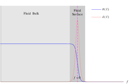
Figure 1: Schematic plots of surface distribution functionals. The dark region denotes surface while the light shaded region denotes the inside of the fluid lump.

Upon variation of the partition function (7) with respect to the background metric, the stress tensor that we get has the form

$$T_{PF}^{\mu\nu}=T_{(0)}^{\mu\nu}\theta(f)+T_{(1)}^{\mu\nu}\tilde{\delta}(f)+T_{(2)}^{\mu\nu\rho}\partial_{\rho}\tilde{\delta}(f)+\dots~{}~{}.$$ (10)

Note that although we were able to remove the derivatives of delta function in the partition function by an integration by parts, such derivatives are still present in the expression for the local stress tensor. The remaining symmetry currents also have a structure similar to (10).

There is a very important and interesting role played by the function $f(x)$ in the partition function (7). We may derive an equation of motion for $f(x)$ by extremizing the partition function with respect to it. We can think of this equation as the one which determines the location of the surface. This equation of motion for $f(x)$ is identical to the particular surface fluid equation which follows by demanding diffeomorphism invariance in directions orthogonal to the surface.

1.1.2 Fluid variables and choice of frames

Now let us consider the description in terms of the original fluid variable $\{u^{\mu},T,\dots\}$. We can write down a stress tensor in terms of these fluid fields and their derivatives purely based on symmetry considerations, which has the same structure as (10), namely

$$T_{C}^{\mu\nu}=\tilde{T}_{(0)}^{\mu\nu}\theta(f)+\tilde{T}_{(1)}^{\mu\nu}\tilde{\delta}(f)+\tilde{T}_{(2)}^{\mu\nu\rho}\partial_{\rho}\tilde{\delta}(f)+\dots~{}~{}.$$ (11)

The transport coefficients are the functions of scalar fluid fields, that multiply specific symmetry structures when $\tilde{T}_{(i)}^{\mu\nu}$ is further expanded in a derivative expansion. The number of scalar structures that goes into the partition function is, in general, much less than the allowed linearly independent symmetry structures which arises in the stress tensor (11). Therefore comparing $T^{C}_{\mu\nu}$ with $T^{PF}_{\mu\nu}$ gives us very non-trivial constraints on the transport coefficients. This exercise, when executed for the fluid configurations with a surface, not only gives relations among surfaces transport coefficients but also relates them with some of the bulk transport coefficients.

While writing (11), there is a crucial issue of the choice of fluid frames. Since we do not want the fluid to spill out of the surface, we must require

$$u^{\mu}n_{\mu}|_{f=0}=0~{}~{},$$ (12)

to be true at all orders in derivative expansion. Also, we want the surface to be moving in the same way as the bulk of the fluid. Therefore a suitable frame choice should ensure that the fluid fields does not jump discontinuously at the surface. We should point out that one of the most popular frame choice - the Landau frame, in which $u^{\mu}$ is an eigen-vector of the full stress tensor, is not a suitable frame choice in this respect. This is because since the stress tensor has new corrections at the surface, the Landau frame choice introduces discontinuities in the fluid variables at the surface. Also, trying to impose the condition (12) in addition to the Landau frame condition may turn out to be more constraining than necessary.

A suggestion for a suitable frame choice may be to work with a Landau frame condition only for the bulk stress tensor. That is, we may impose

$$u^{\mu}\tilde{T}^{(0)}_{\mu\nu}=-\mathcal{E}u_{\nu}~{}~{},$$ (13)

both in the bulk and at the surface of the fluid. Here $\mathcal{E}$ is only the bulk energy density. This, in particular, would imply that the direction of energy flow at the surface of the fluid is not along the fluid flow, which is not a problem at all. However, although this cures one of the problems (that there would be no separate corrections to the fluid fields at the surface), imposing (12) in addition may still be over constraining, particularly at the second and higher orders in derivatives.

This problem may be easier to visualize, if we remember the results of Banerjee:2012iz for 3+1 dimensional uncharged fluids. In that paper, after comparison with the partition function, in the Landau frame, it was found that the velocity $u^{\mu}$, which is identical to the Killing vector of (1) at the leading order, receives nontrivial corrections in terms of derivatives of the background fields at second order in the derivative expansion. So if we now wish to impose (12) on that result, it would be automatically satisfied at the leading and first order. But at second order, it would imply non-trivial constrains involving the background field and the normal vector $n_{\mu}$, which may be too restrictive.

Hence, the most suitable choice of frame for this problem is to choose a frame where (12) is a part of the frame fixing condition. This is possible to implement only because, at leading order the fluid velocity $u^{\mu}$ is proportional to the time-like Killing vector of (1) therefore (12) is automatically satisfied. The higher order corrections can always be manipulated by a frame choice. In fact, we may foliate the bulk of the fluid $\mathcal{M}$, with constant $f(x)$ surfaces, thus extending $n_{\mu}$ throughout $\mathcal{M}$. Then $u^{\mu}n_{\mu}=0$ can be chosen to be part of frame fixing condition throughout the bulk of the fluid. The remaining part of the frame choice can be implemented by imposing a condition similar to (13) but projected orthogonal to $n_{\mu}$. We will refer to this frame as the orthogonal-Landau-frame. While performing the partition function analysis in §3.3, we shall make this frame choice.

There is another very interesting point of view while describing the fluid surface in terms of the fluid variables. We may consider two separate sets of fluids variables one in the bulk $\{u_{\mu},T\}_{\text{blk}}$ and the other at the surface $\{u_{a},T\}_{\text{sur}}$. The surface has one less fluid variable because it is one dimension less than the bulk. Now we can regard the surface equation of motion , as being the dynamical equations for the variables $\{u_{a},T\}_{\text{sur}}$. In this equation, the bulk variables only act as sources and we can solve them to obtain specific solutions $\{u^{\mathfrak{s}}_{a},T^{\mathfrak{s}}\}_{\text{sur}}$. Subsequently we should solve the bulk fluid equations with the boundary condition

$$(u^{\mu}_{\text{blk}})n_{\mu}|_{f=0}=0,~{}\text{and}~{}\{e^{\mu}_{a}u_{\mu},T\}_{\text{blk}}|_{f=0}=\{u^{\mathfrak{s}}_{a},T^{\mathfrak{s}}\}_{\text{sur}}~{}~{},$$ (14)

where $e^{\mu}_{a}$ is the projector on to the tangent space of the surface. Thus, in this point of view, the fluid equations are solved with dynamical boundary conditions. The dynamics of the boundary conditions are given by the surface equations of motion. In this paper, we strive to constrain the form of this surface equation using the framework of the equilibrium partition function.

1.2 A brief summary of results

At first, in §2 we consider perfect fluids in arbitrary dimensions. The partition function for perfect fluids with a surface can be written as

$$\mathcal{W}=\log\mathcal{Z}=\int_{\mathcal{N}_{s}}d^{3}x\sqrt{g}\left(\theta(f)~{}\frac{e^{\sigma}}{T_{0}}~{}\mathcal{P}\left(T_{0}e^{-\sigma}\right)+\tilde{\delta}(f)~{}\frac{e^{\sigma}}{T_{0}}~{}\mathcal{C}\left(T_{0}e^{-\sigma}\right)\right)~{}~{},$$ (15)

where just like $\mathcal{P}$ can be identified with the pressure $P$ in the bulk of the perfect fluid, $\mathcal{C}$ is identified with the surface tension $\chi$. Comparison of the stress tensor constructed through symmetry arguments, with that following from (15) yields the expected surface thermodynamics. The component of the stress tensor conservation equation normal to the surface, at the surface, reads

$$P(T)|_{f=0}=\chi K+T\chi_{S}~{}n_{\mu}\mathfrak{a}^{\mu}|_{f=0}~{}~{},$$ (16)

where $K$ is the extrinsic curvature of the surface and $\mathfrak{a}_{\mu}$ is the fluid acceleration. This is a modified version of the Young-Laplace equation where the term proportional to the acceleration is new compared to its original form. This additional term is non-zero only if the surface entropy $\chi_{S}$ is non-zero, i.e. , if there is a non-trivial temperature dependence of surface tension.

This term has a very simple physical interpretation. If the surface entropy is non-zero, it implies that there are non-trivial degrees of freedom localized at the surface. Then the additional term accounts for the centripetal acceleration of these degrees of freedom in the force balance equation that (16) represents.

Since the acceleration term in (16) has not been widely considered in the literature before, we analyzed the consequence of this term on some simple fluid configurations in §4. For this purpose, as a sample system, we choose to revisit the localized configurations of deconfined plasma of large $N$, strongly coupled $\mathcal{N}=4$ Yang-Mills theory, compatified down to $2+1$ dimensions on a Scherk-Schwarz circle, that were constructed in Lahiri:2007ae . These configurations are dual to exotic black holes in Scherk-Schwarz compactified $AdS_{5}$.

However, due to the unavailability of the exact dependence of surface tension on temperature for this system, the surface tension was taken to be a constant , in the analysis of Lahiri:2007ae . In §4, we suitably parameterized this ignorance and studied the change in the phase diagram for the configurations, as we varied this parameter. We found that turning on this parameter introduced an upper bound on the surface velocity. This arises from the fact that the surface temperature dips below the phase transition temperature, when the bound is overshot. This results in the termination of the phase curve at a specific point, see fig. 2. This has important consequences for the existence of a phase transition between the ball and ring configurations. We find that the phase transition may not exist for large values of this parameter .

Moving on to the case of finite lumps of superfluids, at zeroth order in derivatives, $\mathcal{P}$ and $\mathcal{C}$ in the partition function (15), now would also depend on $A_{0}$ and the norm of the superfluid velocity $\xi_{\mu}$ Bhattacharyya:2012xi . We find that (16) is further modified in the case of superfluids to become

$$P(T)|_{f=0}=\chi K+\left(\chi_{E}-\chi\right)~{}n_{\mu}\mathfrak{a}^{\mu}|_{f=0}+\lambda~{}n^{\mu}~{}\xi^{\nu}~{}\nabla_{\nu}\xi_{\mu}|_{f=0}~{}~{}.$$ (17)

In §3 we consider the case of uncharged fluids in 3+1 dimensions, where the first corrections to the perfect fluid partition function occurs at second order in the bulk and at first order on the surface. The full partition function upto this order, including the parity odd sector, takes the form

$$\begin{split}&\mathcal{W}=\log\mathcal{Z}=\int_{\mathcal{M}_{s}}d^{3}x\sqrt{g}\left(\frac{e^{\sigma}}{T_{0}}~{}\mathcal{P}\left(T_{0}e^{-\sigma}\right)-\frac{1}{2}\bigg{[}P_{1}(\sigma)R+T_{0}^{2}P_{2}(\sigma)f_{ij}f^{ij}+P_{3}(\sigma)(\partial\sigma)^{2}\bigg{]}\right)\\ &+\int_{\partial{\mathcal{M}_{s}}}~{}d^{2}x\sqrt{\gamma}\frac{e^{\sigma}}{T_{0}}\left(~{}\mathcal{C}\left(T_{0}e^{-\sigma}\right)+\mathcal{B}_{1}\left(T_{0}e^{-\sigma}\right)n^{i}~{}\partial_{i}\sigma+\mathcal{B}_{2}\left(T_{0}e^{-\sigma}\right)\epsilon^{ijk}n_{i}f_{jk}+\mathcal{B}_{3}\left(T_{0}e^{-\sigma}\right)\mathcal{K}\right)\bigg{|}_{f=0}~{}~{}.\end{split}$$ (18)

Here $P_{i}$ are the three independent coefficients that were considered in Banerjee:2012iz , while $\mathcal{B}_{i}$ are the new three surface transport coefficients. The terms proportional to $\mathcal{B}_{1}$ and $\mathcal{B}_{2}$ can also be viewed as bulk total derivative terms, while the term $\mathcal{B}_{3}$, a term which was studied in Armas:2013hsa , eventually contributes to the modulus of rigidity.

As pointed out before, the surface transport coefficients in (18) may also depend on $\tilde{\tau}$ (the dimensionless ratio of surface thickness and $T_{0}$), which we leave implicit here. If any particular limit is taken on this parameter $\tilde{\tau}$, it may directly influence the surface transport coefficients in (18), particularly $\mathcal{B}_{3}$.

For the stress tensor $T_{C}^{\mu\nu}$, which follows from symmetry considerations, there are 31 surface terms that can be written down, which are linearly independent for stationary configurations. Now, taking into consideration the fact that $P_{i}$ correspond to three independent transport coefficient in the bulk fluid, we are able to derive 28 relations between the 31 surface transport coefficients and the 3 independent bulk transport coefficients, as it has been explicated in §3.

2 Perfect fluids

In this section we will study fluids at zeroth order in derivatives. At this order, the only surface effect is encoded in the surface tension, which is extremely well studied. However, it is very instructive to re-derive the known physics in the language of partition functions described in §1. We will also get the occasions to discuss a few effects related to the temperature dependence of surface tension and surface tension in superfluids which has not been widely discussed in the literature.

2.1 Ordinary uncharged perfect fluids in arbitrary dimensions

At first, let us briefly review the partition function for space filling ordinary perfect fluids as discussed in Banerjee:2012iz . The partition function in terms of the metric sources can be written as,

$$\mathcal{W}=\log\mathcal{Z}=\int d^{3}x\sqrt{g}~{}\frac{e^{\sigma}}{T_{0}}~{}\mathcal{P}\left(T_{0}e^{-\sigma}\right)~{}~{}.$$ (19)

The functional form of $\mathcal{P}$ is to be determined from microscopics. Let us now evaluate the stress tensor from the above partition function by using Banerjee:2012iz

$$T_{00}=-\frac{T_{0}e^{2\sigma}}{\sqrt{-\cal G}}\frac{\delta\mathcal{W}}{\delta\sigma}~{}~{},~{}~{}T_{0}^{i}=\frac{T_{0}}{\sqrt{-\cal G}}\frac{\delta\mathcal{W}}{\delta a_{i}}~{}~{},~{}~{}T^{ij}=-\frac{2T_{0}}{\sqrt{-\cal G}}g^{il}g^{jm}\frac{\delta\mathcal{W}}{\delta g^{lm}}~{}~{}.$$ (20)

Evaluating these formulae explicitly for (19) we get

$$T_{00}=e^{2\sigma}\left(\mathcal{P}-T\frac{\partial\mathcal{P}}{\partial T}\right)~{}~{},~{}T_{0}^{i}=0~{},~{}T^{ij}=\mathcal{P}g^{ij}~{}~{},$$ (21)

where $T=T_{0}~{}e^{-\sigma}$. By comparing (21) with the zeroth order form of the stress tensor that follows from symmetry considerations

$$T_{\mu\nu}=\left(\mathcal{E}(T)+P(T)\right)u_{\mu}u_{\nu}+P(T)\mathcal{G}_{\mu\nu}+\dots~{}~{},$$ (22)

we get

$$P=\mathcal{P}~{},~{}\mathcal{E}=-\mathcal{P}+T\frac{\partial\mathcal{P}}{\partial T}~{}~{},$$ (23)

while the fluids fields are found to be

$$u^{\mu}=e^{-\sigma}\{1,0,\dots,0\}+\dots~{}~{},~{}~{}T=T_{0}e^{-\sigma}+\dots~{}~{}.$$ (24)

Note that (23) is identical to the condition on pressure and energy density that follows from thermodynamics. In this way, we are able to derive the thermodynamic properties of the fluid by comparison with the partition function. In some sense, pressure and energy density can be thought of as zeroth order transport coefficients, which are related by thermodynamic relations which follow from the partition function analysis.

Following the above procedure, we wish to write down a partition function for perfect fluids in equilibrium, confined within a surface (which itself is dynamically determined by minimization of the free energy). Respecting the principles of KK-gauge invariance for writing down the partition function and reparameterization invariance of the surface, the partition function is given in terms of two unknown functions

$$\mathcal{W}=\log\mathcal{Z}=\int_{\mathcal{N}_{s}}d^{3}x\sqrt{g}\left(\theta(f)~{}\frac{e^{\sigma}}{T_{0}}~{}\mathcal{P}\left(T_{0}e^{-\sigma}\right)+\tilde{\delta}(f)~{}\frac{e^{\sigma}}{T_{0}}~{}\mathcal{C}\left(T_{0}e^{-\sigma}\right)\right)~{}~{}.$$ (26)

In order to obtain the stress tensor, we have to vary the partition function (26) with respect to the background metric fields .

In fact, using (20), explicitly we find

$$\begin{split}T_{00}&=e^{2\sigma}\left(\mathcal{P}-T\frac{\partial\mathcal{P}}{\partial T}\right)\theta(f)+\tilde{\delta}(f)e^{2\sigma}\left(\mathcal{C}-T\frac{\partial\mathcal{C}}{\partial T}\right)~{}~{},\\ T_{0}^{i}&=0~{}~{},\\ T^{ij}&=\mathcal{P}g^{ij}\theta(f)+\tilde{\delta}(f)\mathcal{C}\gamma^{ij}~{}~{}.\end{split}$$ (27)

Now we have to compare (27) with the stress tensor that may be written from symmetry arguments (11) to this particular order, namely,

$$T_{\mu\nu}=T_{\mu\nu}^{(0)}\theta(f)+T_{\mu\nu}^{(1)}\tilde{\delta}(f)~{}~{}.$$ (28)

The bulk stress tensor components $T_{\mu\nu}^{(0)}$ are given by (22), while the components of the surface stress tensor also have a similar form

$$T_{\mu\nu}^{(1)}=\chi_{E}(T)~{}u_{\mu}u_{\nu}-\chi(T)~{}\mathcal{P}_{\mu\nu}+\dots~{}~{}.$$ (29)

Here, $\mathcal{P}_{\mu\nu}=\mathcal{G}_{\mu\nu}+u_{\mu}u_{\nu}-n_{\mu}n_{\nu}$ is the projector orthogonal to both the velocity vector and the normal to the surface. In (29) we also introduced $\chi_{E}$ and $\chi$, which are, respectively, the surface energy and the surface ‘pressure’, also known as surface tension.

Comparing (27) with (29), we can therefore identify

$$\chi=-\mathcal{C}~{}~{},~{}~{}\chi_{E}=-\mathcal{C}+T\frac{\partial\mathcal{C}}{\partial T}~{}~{},$$ (30)

while the fluids fields are again given by (24). This identification (30) had also been done in Armas:2013hsa . Just like the bulk perfect fluid, (30) implies the thermodynamic identity

$$\chi_{E}=\chi+T\chi_{S}~{}~{},$$ (31)

where $\chi_{S}=-\partial\chi/\partial T$ is the surface entropy. Therefore, if the surface tension depends non-trivially on the fluid temperature, it means that the surface entropy is non-zero and hence that there are active degrees of freedom living on the surface of the fluid. When the surface entropy vanishes (that is the surface tension is constant), the surface tension is equal to the negative of surface energy.

The conservation of the stress tensor (28), implies

$$\nabla_{\mu}T^{\mu\nu}=\theta(f)\nabla_{\mu}T^{\mu\nu}_{(0)}+\delta(f)\left(-n_{\mu}T^{\mu\nu}_{(0)}+\tilde{\nabla}_{\mu}T^{\mu\nu}_{(1)}\right)+\dots~{}~{},$$ (32)

where we have defined $\tilde{\nabla}_{\mu}\left(\dots\right)=1/\sqrt{\partial f\cdot\partial f}~{}~{}\nabla_{\mu}\left(\sqrt{\partial f\cdot\partial f}\dots\right)$. In the bulk (32) will give rise to the usual equation bulk conservation equation $\nabla_{\mu}T^{\mu\nu}_{(0)}$, while at the surface, it gives rise to the condition

$$-n_{\mu}T^{\mu\nu}_{(0)}|_{f=0}+\tilde{\nabla}_{\mu}T^{\mu\nu}_{(1)}=0~{}~{}.$$ (33)

This equation is in fact a Carter equation with a force term Carter:2000wv , and is extensively used in the context of (mem)-brane hydrodynamics Emparan:2009at ; Armas:2013hsa ; Armas:2013goa ; Armas:2014rva . As with any Carter equation, (33) gives rise to two physically different sets of equations, obtained by projecting both orthogonally and tangentially to the fluid surface. Before doing so, let us note that

$$n_{\mu}T^{\mu\nu}_{(0)}=n^{\nu}P(T)|_{f=0}~{}~{},$$ (34)

that is, for a perfect fluid, the bulk contribution to (33) is only present in the normal component of (33). Thus, if we project (33) along the fluid surface with the projector $e^{a}_{\nu}$ such that $n^{\nu}e^{a}_{\nu}=0$, we obtain

$$e^{a}_{\nu}\tilde{\nabla}_{\mu}T^{\mu\nu}_{(1)}=0~{}~{}.$$ (35)

Here the index $a=0,1,2$ labels the directions along the surface. Equation (35) expresses the conservation of the surface stress tensor along the surface. Note that if we consider higher derivative corrections, this equation will also receive a contribution from the bulk stress tensor, which would signify energy and momentum transport from the bulk to the surface. For the perfect fluid, however, such transport does not take place.

The component of (33) normal to the surface, describing the elastic degrees of freedom of the surface, is more interesting and provides us with the condition that determines the position of the surface. For perfect fluids, it reduces to

$$-P(T)|_{f=0}+n_{\nu}\tilde{\nabla}_{\mu}T^{\mu\nu}_{(1)}=0~{}~{}.$$ (36)

Now, given that the surface stress tensor (29) is orthogonal to the normal vector $n_{\mu}$, we can rewrite the second term in (36) in the following way

$$P(T)|_{f=0}+T^{\mu\nu}_{(1)}K_{\mu\nu}=0~{}~{},$$ (37)

where $K_{\mu\nu}$ is the extrinsic curvature of the surface. We can easily check that both (36) and (37) reduces to

$$P(T)|_{f=0}=\chi K+\left(\chi_{E}-\chi\right)~{}n_{\mu}\mathfrak{a}^{\mu}|_{f=0}~{}~{},$$ (38)

where $\mathfrak{a}_{\mu}=u^{\nu}\nabla_{\nu}u_{\mu}$ is the fluid acceleration, and $K=\mathcal{G}^{\mu\nu}K_{\mu\nu}$ is the mean extrinsic curvature. If there are no active degrees of freedom in the boundary and the surface tension is constant implying that $\chi_{E}=\chi$, then (38) immediately reduces to

$$P(T)|_{f=0}=\chi K~{}~{},$$ (39)

which is the Young-Laplace equation. Thus (38) is a generalization of the Young-Laplace equation, when there are non-trivial degrees of freedom living on the surface of the fluid. Such generalization had not been previously considered in the works of Lahiri:2007ae ; Caldarelli:2008mv ; Bhattacharya:2009gm . In §4, we shall examine the consequence of the presence of this additional term in (38) for some simple fluid configurations.

It is noteworthy that (38) can also be directly obtained from the partition function (26). In terms of the partition function, this is simply given by the extremization of the partition function with respect to the surface function $f$, which is the equation of motion $f$. This is intuitively expected since the location of the fluid surface is obtained by the minimization of the free energy. If we vary (26) with respect to $f$, at the leading order we find

$$\delta(f)\left(\mathcal{P}+\mathcal{C}(T_{0}e^{-\sigma})\mathcal{K}+\left(\mathcal{C}(T_{0}e^{-\sigma})-\mathcal{T}~{}\frac{\partial\mathcal{C}(T_{0}e^{-\sigma})}{\partial\mathcal{T}}\right)~{}n^{i}\partial_{i}\sigma\right)=0~{}~{},$$ (40)

where $\mathcal{K}=g^{ij}\bar{\nabla}_{i}n_{j}$, with $\bar{\nabla}$ being the spatial covariant derivative defined with respect to the reduced metric . Given the thermodynamical relations (23), (30) and remembering that in terms of the background fields the fluid acceleration is given by $\mathfrak{a}^{i}=g^{ij}\partial_{j}\sigma$ Banerjee:2012iz , (38) reduces to (40).

2.2 Zeroth order superfluids with a surface

For the case of superfluids, the zeroth order stress tensor is modified in order to include the superfluid velocity $\xi_{\mu}$ Landau:1941 ; Tisza:1947zz . The bulk stress tensor has the form

$$T_{\mu\nu}^{(0)}=(\epsilon+P)u_{\mu}u_{\nu}+P\mathcal{G}_{\mu\nu}+\lambda\xi_{\mu}\xi_{\nu}~{}~{},$$ (41)

and it is accompanied by a conserved current

$$J_{\mu}^{(0)}=qu_{\mu}-\lambda\xi_{\mu}~{}~{}.$$ (42)

Just like in the case of ordinary fluids, in the presence of a surface there are surface stress tensor and current contributions, which read

$$\begin{split}T^{(1)}_{ab}&=(\epsilon+P)u_{a}u_{b}+P\mathcal{H}_{ab}+\lambda\xi_{a}\xi_{b}~{}~{},~{}~{}J^{(1)}_{a}=q~{}u_{a}-\lambda~{}\xi_{a}~{}~{}.\end{split}$$ (43)

It can be explicitly checked that this form of the boundary stress tensor and current follows from the following partition function

$$\mathcal{W}=\log\mathcal{Z}=\int_{\mathcal{M}}d^{3}x\sqrt{g}\frac{e^{\sigma}}{T_{0}}~{}\mathcal{P}\left(T_{0}e^{-\sigma},A_{0},\xi\right)+\int_{\partial{\mathcal{M}}}~{}d^{2}x\sqrt{\gamma}\frac{e^{\sigma}}{T_{0}}~{}\mathcal{C}\left(T_{0}e^{-\sigma},A_{0},\xi\right)\bigg{|}_{f=0}~{}~{},$$ (44)

where $\xi$ is the norm of the superfluid velocity. The bulk term of this partition function was first derived in Bhattacharyya:2012xi . In the presence of the surface we must also assume that the superfluid velocity and the normal to the surface are mutually orthogonal $n^{\mu}\xi_{\mu}|_{f=0}=0$. As in the previous sections, the stress tensor is conserved and the normal component of the conservation of the boundary stress tensor gives the generalized Young-Laplace equation. To leading order, the bulk and surface currents are conserved separately, with no current flowing from the bulk to the surface.

The generalized Laplace-Young equation (38), is further modified in the case of superfluids. It takes the form

$$P(T)|_{f=0}=\chi K+\left(\chi_{E}-\chi\right)~{}n_{\mu}\mathfrak{a}^{\mu}|_{f=0}+\lambda~{}n^{\mu}~{}\xi^{\nu}~{}\nabla_{\nu}\xi_{\mu}|_{f=0}~{}~{}.$$ (45)

Note that the new term is present even if there is no temperature dependence in the surface tension, as long as the goldstone boson also constitutes an active degree of freedom on the surface. Also this modified equation is also applicable to the case when there is an emergent goldstone boson only at the surface of a fluid, a situation which is reminiscent of topological insulators in the context of fluids.

3 Next to leading order corrections for uncharged fluids

In this section we shall consider the next to leading order corrections for uncharged fluids with a surface. The principal goal of this section is to demonstrate that there are only three new equilibrium transport coefficients on the surface of the uncharged fluid, at the next to leading order, two of which are parity even and the other one being parity odd. Two of these new boundary terms in the partition function, also precisely coincide with two possible bulk total derivative terms. Here, we work out the interplay between these new surface transport coefficients and the bulk second order transport coefficients.

3.1 Partition function at next to leading order

In order to write down the first corrections to the partition function (26), we need to write down all KK-gauge invariant scalar terms at higher order in derivatives. As it was observed in Banerjee:2012iz , the bulk of the fluid does not receive any corrections at first order. In other words, there are no KK-gauge invariant scalar bulk terms at first order, which can be written in terms of the sources of an uncharged fluid.

However, at the surface of the fluid, there is an additional geometrical structure, which is the vector normal to the fluid surface. This allows us to write down two possible parity even scalar terms which may constitute the partition function. These are

$$\mathcal{K}~{}~{},~{}~{}n_{i}~{}\partial^{i}\sigma~{}~{}.$$ (46)

Here $\mathcal{K}$ is the trace of the extrinsic curvature reduced along the time direction

Now for parity odd terms, there is only one possible parity odd scalar

$$\epsilon^{ijk}n_{i}f_{jk}~{}~{},$$ (47)

which must be taken into account while writing down the partition function. For space-filling fluids, it was not possible to construct any parity odd term in the partition function, at the second order Banerjee:2012iz . Therefore the existence of this term suggests that even uncharged fluids may have parity odd transport when surface effects are considered. Since, the fluid surface is co-dimension one, this term is particularly reminiscent of a parity odd transport that can exist in $2+1$ dimensions Banerjee:2012iz ; Jensen:2012jh .

Including these new surface terms, the partition function takes the following form

$$\begin{split}&\mathcal{W}=\log\mathcal{Z}=\int_{\mathcal{M}_{s}}d^{3}x\sqrt{g}\left(\frac{e^{\sigma}}{T_{0}}~{}\mathcal{P}\left(T_{0}e^{-\sigma}\right)\right)\\ &+\int_{\partial{\mathcal{M}_{s}}}~{}d^{2}x\sqrt{\gamma}\frac{e^{\sigma}}{T_{0}}\left(~{}\mathcal{C}\left(T_{0}e^{-\sigma}\right)+\mathcal{B}_{1}\left(T_{0}e^{-\sigma}\right)n^{i}~{}\partial_{i}\sigma+\mathcal{B}_{2}\left(T_{0}e^{-\sigma}\right)\epsilon^{ijk}n_{i}f_{jk}+\mathcal{B}_{3}\left(T_{0}e^{-\sigma}\right)\mathcal{K}\right)\bigg{|}_{f=0}~{}.\end{split}$$ (48)

It is important to note that if we include these first order surface terms in the partition function then we must also include the second order bulk terms for consistency. For instance, the surface stress tensor following from the partition function in (48) may get contributions from total derivative terms at second order in the bulk. In fact, we must point out that two of the new terms that we have added in (48) may also be written as a bulk total derivative terms at second order.

Thus, including the bulk second order terms, which was written down in Banerjee:2012iz , we have

$$\begin{split}&\mathcal{W}=\log\mathcal{Z}=\int_{\mathcal{M}_{s}}d^{3}x\sqrt{g}\left(\frac{e^{\sigma}}{T_{0}}~{}\mathcal{P}\left(T_{0}e^{-\sigma}\right)-\frac{1}{2}\bigg{[}P_{1}(\sigma)R+T_{0}^{2}P_{2}(\sigma)f_{ij}f^{ij}+P_{3}(\sigma)(\partial\sigma)^{2}\bigg{]}\right)\\ &+\int_{\partial{\mathcal{M}_{s}}}~{}d^{2}x\sqrt{\gamma}\frac{e^{\sigma}}{T_{0}}\left(~{}\mathcal{C}\left(T_{0}e^{-\sigma}\right)+\mathcal{B}_{1}\left(T_{0}e^{-\sigma}\right)n^{i}~{}\partial_{i}\sigma+\mathcal{B}_{2}\left(T_{0}e^{-\sigma}\right)\epsilon^{ijk}n_{i}f_{jk}+\mathcal{B}_{3}\left(T_{0}e^{-\sigma}\right)\mathcal{K}\right)\bigg{|}_{f=0}~{},\end{split}$$ (49)

where $P_{i}$ denote the three independent transport coefficients at second order for a fluid without surfaces.

Now, as pointed out before we can write the new surface terms as a bulk term in the following way

$$\begin{split}\mathcal{W}=\log\mathcal{Z}=&\int_{\mathcal{M}_{s}}d^{3}x\sqrt{g}\left(\frac{e^{\sigma}}{T_{0}}~{}\mathcal{P}\left(T_{0}e^{-\sigma}\right)\right.\\ &\left.-\frac{1}{2}\bigg{[}P_{1}(\sigma)R+T_{0}^{2}P_{2}(\sigma)f_{ij}f^{ij}+P_{3}(\sigma)(\partial\sigma)^{2}+\nabla^{2}P_{4}(\sigma)+\epsilon^{ijk}\left(\partial_{i}P_{5}\right)f_{jk}\bigg{]}\right)\\ &+\int_{\partial{\mathcal{M}_{s}}}~{}d^{2}x\sqrt{\gamma}\left(\frac{e^{\sigma}}{T_{0}}~{}\mathcal{C}\left(T_{0}e^{-\sigma}\right)+P_{6}(\sigma)\mathcal{K}\right)\bigg{|}_{f=0}~{},\end{split}$$ (50)

where we have defined

$$\begin{split}P_{4}^{\prime}(\sigma)&=-\frac{2e^{\sigma}}{T_{0}}\mathcal{B}_{1}\left(T_{0}e^{-\sigma}\right)~{}~{},~{}~{}P_{5}(\sigma)=-\frac{2e^{\sigma}}{T_{0}}\mathcal{B}_{2}\left(T_{0}e^{-\sigma}\right)~{}~{},~{}~{}P_{6}(\sigma)=\frac{e^{\sigma}}{T_{0}}\mathcal{B}_{3}\left(T_{0}e^{-\sigma}\right)~{}~{}.\end{split}$$ (51)

Now, as it was shown in Banerjee:2012iz , $P_{1},P_{2}$ and $P_{3}$ were determined in terms of the bulk second order equilibrium coefficients. Also eliminating the $P_{1},P_{2}$ and $P_{3}$ from those relations, gave rise to 5 relations among the eight possible second order equilibrium transport coefficients.

It is clear that the terms proportional to $P_{4}$ and $P_{5}$ (or any total derivative term) will not enter the bulk stress tensor . But they definitely contribute non-trivially to the surface stress tensor. It is important to note that both the form of the partition function (49) and (50) are equivalent and describe the same system. Hence, everything physical that is evaluated from them, such as the surface stress tensor or the Young-Laplace equation, must be identical.

3.2 Corrections to the stress tensor

Once we have written down the partition function (50), it is immediate to evaluate the stress tensor by varying with respect to the background fields using (20). It is convenient to split the bulk and surface contributions, up to second order, in the followind way

$$T^{\mu\nu}_{\text{blk}}=T^{\mu\nu}_{(0)}\theta(f)~{}~{},~{}~{}T^{\mu\nu}_{\text{sur}}=T^{\mu\nu}_{(1)}\tilde{\delta}(f)+T^{\mu\nu\rho}_{(2)}\partial_{\rho}\tilde{\delta}(f)~{}~{}.$$ (53)

The bulk stress tensor remains the same as that computed in Banerjee:2012iz and involves only the the coefficients $P_{1},P_{2}$ and $P_{3}$ while the surface contribution is obtained as terms proportional to $\tilde{\delta}(f)$ and its derivatives

$$\begin{split}{T_{\text{sur}}}^{lk}&=g^{li}g^{kj}\Bigg{[}\tilde{\delta}(f)T_{0}e^{-\sigma}\bigg{[}g_{ij}\left(-P_{1}\mathcal{K}-\left(2P^{\prime}_{1}+\frac{1}{2}P_{4}^{\prime}+{P^{\prime}_{6}}\right)n^{k}\partial_{k}\sigma\right)\\ &-n_{i}n_{j}\left({P^{\prime}_{6}n^{k}\partial_{k}\sigma+P_{6}\mathcal{K}}\right)+P_{1}\nabla_{(i}n_{j)}+(2P^{\prime}_{1}+P^{\prime}_{4}+{2P^{\prime}_{6}})n_{(i}\partial_{j)}\sigma\bigg{]}\\ &+T_{0}e^{-\sigma}\bigg{[}(P_{1}+{2P_{6}})n_{(i}\partial_{j)}\tilde{\delta}(f)-(P_{1}+{P_{6}})g_{ij}n^{k}\partial_{k}\tilde{\delta}(f)-{P_{6}n_{i}n_{j}n^{k}\partial_{k}\tilde{\delta}(f)}\bigg{]}\Bigg{]}~{}~{},\\ {T^{\text{sur}}_{00}}&=\tilde{\delta}(f)T_{0}e^{\sigma}\bigg{[}(-\frac{1}{2}P^{\prime}_{4}+{P^{\prime}_{6}})\mathcal{K}+P_{3}~{}n^{k}\partial_{k}\sigma+\frac{1}{2}P^{\prime}_{5}~{}\epsilon^{ijk}n_{i}f_{jk}\bigg{]}+\left(-\frac{1}{2}T_{0}e^{\sigma}P^{\prime}_{4}\right)~{}n^{k}\partial_{k}\tilde{\delta}(f)~{}~{},\\ {T_{\text{sur}}}^{i}_{0}&=\tilde{\delta}(f)\bigg{[}-T_{0}^{3}e^{-\sigma}P_{2}n_{j}f^{ji}+T_{0}e^{-\sigma}\epsilon^{ijk}\left(P^{\prime}_{5}n_{j}\partial_{k}\sigma\right)\bigg{]}~{}~{}.\end{split}$$ (54)

This stress tensor must satisfy the conservation equation

$$\nabla_{\mu}T^{\mu\nu}_{\text{sur}}=T^{\mu\nu}_{(0)}n_{\mu}\tilde{\delta}(f)~{}~{},$$ (55)

which gives rise to two separate sets of equations as in §2, one determining the position of the surface and the other the conservation of the surface stress tensor along surface directions. Indeed, by explicitly using (54), one can verify that the tangential projection of (55) is automatically verified - a trivial consequence of diffeomorphism invariance along the surface.

3.3 Constraints on surface transport coefficients from the equilibrium partition function

In this section we write down the next to leading order surface stress tensor in equilibrium by classifying all the terms allowed by symmetries. We then reduce this stress tensor along the time circle and compare it with that which follows from the partition function. This allows us to see a rich interplay between the surface transport coefficients and the bulk second order coefficients.

$a$	$\mathcal{S}_{(a)}$	Reduced form $\mathcal{S}_{(a)}^{\text{red}}$
1	$\tilde{\delta}(f)~{}n^{\mu}\mathfrak{a}_{\mu}$	$\tilde{\delta}(f)~{}n^{i}\partial_{i}\sigma$
2	$\tilde{\delta}(f)~{}K$	$\tilde{\delta}(f)\left(\mathcal{K}+n^{i}\partial_{i}\sigma\right)$
3	$\tilde{\delta}(f)~{}n^{\mu}\ell_{\mu}$	$\tilde{\delta}(f)~{}\left(\frac{e^{\sigma}}{2}\right)\epsilon^{ijk}n_{i}f_{jk}$
4	$n^{\mu}\partial_{\mu}\tilde{\delta}(f)$	$n^{i}\partial_{i}\tilde{\delta}(f)$

Table 1: Scalars

$a$	$\mathcal{V}^{\mu}_{(a)}$	Reduced form $\mathcal{V}^{i}_{(a)}$
1	$\tilde{\delta}(f)~{}\mathcal{P}^{\mu\alpha}\mathfrak{a}_{\alpha}$	$\tilde{\delta}(f)~{}\mathcal{P}^{ij}\partial_{j}\sigma$
2	$\tilde{\delta}(f)~{}\mathcal{P}^{\mu\alpha}n^{\nu}\omega_{\nu\alpha}$	$\tilde{\delta}(f)~{}\left(\frac{e^{\sigma}}{2}\right)\mathcal{P}^{ij}f_{jk}n^{k}$
3	$\tilde{\delta}(f)~{}\mathcal{P}^{\mu\alpha}n^{\beta}\nabla_{\beta}n_{\alpha}$	$\tilde{\delta}(f)~{}\mathcal{P}^{ij}n^{k}\nabla_{k}n_{j}$
4	$\tilde{\delta}(f)~{}\mathcal{P}^{\mu\alpha}\ell_{\alpha}$	$\tilde{\delta}(f)~{}\left(\frac{e^{\sigma}}{2}\right)\mathcal{P}^{ij}g_{jk}\epsilon^{klm}f_{lm}$
5	$\tilde{\delta}(f)~{}\mathcal{P}^{\mu\alpha}\epsilon_{\alpha\lambda\nu\sigma}u^{\lambda}n^{\nu}\mathfrak{a}^{\sigma}$	$\tilde{\delta}(f)~{}\mathcal{P}^{ij}g_{jk}\epsilon^{klm}n_{l}\partial_{m}\sigma$
6	$\tilde{\delta}(f)~{}\mathcal{P}^{\mu\alpha}\epsilon_{\alpha\nu\lambda\sigma}u^{\nu}\nabla^{\lambda}n^{\sigma}$	$\tilde{\delta}(f)~{}\mathcal{P}^{ij}g_{jk}\epsilon^{klm}\nabla_{l}n_{m}$
7	$\mathcal{P}^{\mu\alpha}\partial_{\alpha}\tilde{\delta}(f)$	$\mathcal{P}^{ij}\partial_{j}\tilde{\delta}(f)$

Table 2: The first order vectors on the surface projected on the surface and orthogonal to the velocities. Here $\mathcal{P}^{\mu\nu}=\mathcal{G}^{\mu\nu}+u^{\mu}u^{\nu}-n^{\mu}n^{\nu}$, is the projector orthogonal to both $u^{\mu}$ and $n^{\mu}$. The spatial components of this projector, projects orthogonal to $n^{i}$ in a given time slice, that is $\mathcal{P}^{ij}=g^{ij}-n^{i}n^{j}$. Also, note that in the reduced language ${\mathcal{V}_{0}}^{(j)}=0$.

Under the assumption of time independence, at first order on the surface, the non-zero linearly independent terms have been classified in Tables 1, 2 and 3. The presence of the vectors $u_{\mu}$ and $n_{\mu}$ breaks down the local Lorentz symmetry at the surface to a smaller subgroup. The classification is based on transformation properties of the surface quantities under this preserved subgroup. We refer to the objects as scalars, vectors and tensors, depending on their transformation properties under this subgroup. Note that we have defined $K_{\mu\nu}=\nabla_{(\mu}n_{\nu)}$.

We would like to point out that in Table 2, we have not included the term $\mathcal{P}^{\mu\alpha}u^{\beta}\nabla_{\beta}n_{\alpha}$ because upon reduction it evaluates to the same result as $\mathcal{P}^{\mu\alpha}n^{\nu}\omega_{\nu\alpha}$. Hence, in the stationary equilibrium case under consideration, these two terms are not independent. Also, owing to the identity

$$\epsilon^{ijk}n_{j}\partial_{k}\tilde{\delta}(f)=\tilde{\delta}(f)\epsilon^{ijk}\partial_{j}n_{k}~{}~{},$$

the term $\mathcal{P}^{\mu\alpha}\epsilon_{\alpha\nu\lambda\sigma}n^{\nu}u^{\lambda}\nabla^{\sigma}\tilde{\delta}(f)$ is not independent from $V^{\mu}_{(6)}$. Also note that in Table 3, $P^{\alpha\beta}K_{\alpha\beta}$ is distinct from $K$, since $u^{\alpha}u^{\beta}K_{\alpha\beta}$ is non-zero. In the stationary case, $P^{\alpha\beta}K_{\alpha\beta}$ reduces to $\mathcal{K}$, while $K=\mathcal{K}+n\cdot\partial\sigma$, as shown in Table 1.

$k$	$\mathcal{T}^{\mu\nu}_{(k)}$	Reduced form $\mathcal{T}^{ij}_{(k)}$
1	$\mathcal{P}^{\mu\alpha}\mathcal{P}^{\nu\beta}K_{\alpha\beta}-\frac{1}{2}\mathcal{P}^{\mu\nu}\mathcal{P}^{\alpha\beta}K_{\alpha\beta}$	$\mathcal{P}^{ik}\mathcal{P}^{jm}\left(\mathcal{K}_{km}-\frac{1}{2}g_{km}\mathcal{K}\right)$

Table 3: Symmetric traceless tensor. Upon reduction, $\mathcal{T}^{i}_{0}$ and $\mathcal{T}_{00}$ components of the tensor vanishes.

Since we would like to have, the velocity at the surface, to be equal to the bulk velocity evaluated at the surface, there is no freedom in choosing a frame at the surface once the bulk frame has been chosen, as discussed in §1.1.2. In order to respect the continuity of fluid variables and to naturally impose the condition (12), we shall proceed with the frame choice as described in §1.1.2. This frame choice only constrains the form of the bulk stress tensor and leaves the surface stress tensor unconstrained. Therefore, while constructing the surface stress tensor at first order, we have to write down all possible terms that are allowed by symmetry without imposing any restrictions. We have

$$\begin{split}T_{\text{sur}}^{\mu\nu}=&~{}\sum_{i=1}^{4}\left(\mathcal{P}^{\mu\nu}~{}{\mathfrak{s1}}_{i}~{}\mathcal{S}_{(i)}+u^{\mu}u^{\nu}~{}{\mathfrak{s2}}_{i}~{}\mathcal{S}_{(i)}+n^{\mu}n^{\nu}~{}{\mathfrak{s3}}_{i}~{}\mathcal{S}_{(i)}+u^{(\mu}n^{\nu)}~{}{\mathfrak{s4}}_{i}~{}\mathcal{S}_{(i)}\right)\\ &+\sum_{i=1}^{7}2\left(\mathfrak{v1}_{i}~{}u^{(\mu}\mathcal{V}^{\nu)}_{(i)}+\mathfrak{v2}_{i}~{}n^{(\mu}\mathcal{V}^{\nu)}_{(i)}\right)+{\mathfrak{t}}\mathcal{T}^{\mu\nu}~{}~{},\end{split}$$ (56)

where $\{\mathcal{S}_{(i)},\mathcal{V}^{\nu}_{(i)},\mathcal{T}^{\mu\nu}\}$ are specified in the second column of Tables 1, 2 and 3, respectively. The corresponding surface transport coefficients are denoted by $\{\mathfrak{s1}_{i},\mathfrak{s2}_{i},\mathfrak{s3}_{i},\mathfrak{s4}_{i},\mathfrak{v1}_{i},\mathfrak{v2}_{i},\mathfrak{t}\}$. As we may already foresee, among these $4\times 4+2\times 7+1=31$ transport coefficients, only 3 are independent. The rest are determined in terms one another or bulk second order transport coefficients. We will now work out these relations.

If we consider the reduction of (56) along the time direction, we obtain the following reduced stress tensor

$$\begin{split}&{T^{\text{sur}}}_{00}=\sum_{a=1}^{4}e^{2\sigma}~{}{\mathfrak{s2}}_{a}~{}\mathcal{S}_{(a)}^{\text{red}}~{}~{},\\ &{T_{\text{sur}}}_{0}^{i}=\sum_{a=1}^{4}\left(-e^{\sigma}\right)n^{i}~{}{\mathfrak{s4}}_{a}~{}\mathcal{S}_{(a)}^{\text{red}}+\sum_{a=1}^{7}\left(-e^{\sigma}\right)\mathfrak{v1}_{a}\mathcal{V}^{i}_{(a)}~{}~{},\\ &{T_{\text{sur}}}^{ij}=\sum_{a=1}^{4}\left(\mathcal{P}^{ij}~{}{\mathfrak{s1}}_{a}~{}\mathcal{S}_{(a)}^{\text{red}}+n^{i}n^{j}~{}{\mathfrak{s3}}_{a}~{}\mathcal{S}_{(a)}^{\text{red}}\right)+\sum_{a=1}^{7}\left(\mathfrak{v2}_{a}~{}n^{(i}\mathcal{V}^{j)}_{(a)}\right)+{\mathfrak{t}}~{}\mathcal{T}^{ij}~{}~{},\\ \end{split}$$ (57)

where $\{\mathcal{S}_{(a)}^{\text{red}},V^{i}_{(a)},\mathcal{T}^{ij}\}$ are specified in the third column of Tables 1, 2 and 3, respectively.

Now comparing (57) with (54) we get

$$\begin{split}&\mathfrak{s2}_{1}=T_{0}e^{-\sigma}\left(P_{3}+\frac{1}{2}P_{4}^{\prime}-P_{6}^{\prime}\right),~{}\mathfrak{s2}_{2}=T_{0}e^{-\sigma}\left(-\frac{1}{2}P_{4}^{\prime}+P_{6}^{\prime}\right),~{}\mathfrak{s2}_{3}=T_{0}e^{-2\sigma}P_{5}^{\prime},~{}\mathfrak{s2}_{4}=-\frac{T_{0}e^{-\sigma}}{2}P_{4}^{\prime},\\ &\mathfrak{s4}_{a}=0,~{}\forall a\in\{1,2,3,4\},\mathfrak{v1}_{a}=0,~{}\forall a\in\{1,4,3,6,7\},\mathfrak{v1}_{2}=2(T_{0}^{3}e^{-3\sigma})P_{2},\mathfrak{v1}_{5}=\left(-T_{0}e^{-2\sigma}P_{5}^{\prime}\right),\\ &\mathfrak{v2}_{a}=0,~{}\forall a\in\{2,4,5,6\},\mathfrak{v2}_{1}=T_{0}e^{-\sigma}\left(2P_{1}^{\prime}+P_{4}^{\prime}+2P_{6}^{\prime}\right),~{}\mathfrak{v2}_{3}=T_{0}e^{-\sigma}P_{1},\\ &\mathfrak{v2}_{7}=T_{0}e^{-\sigma}\left(P_{1}+2P_{6}\right),\mathfrak{s1}_{1}=T_{0}e^{-\sigma}\left(P_{1}-\left(2P_{1}^{\prime}+\frac{1}{2}P_{4}^{\prime}+P_{6}^{\prime}\right)\right),~{}\mathfrak{s1}_{2}=-T_{0}e^{-\sigma}P_{1},~{}\mathfrak{s1}_{3}=0,\\ &\mathfrak{s1}_{4}=-T_{0}e^{-\sigma}\left(P_{1}+P_{6}\right),~{}\mathfrak{s3}_{1}=T_{0}e^{-\sigma}\left(P_{1}+P_{6}+\frac{1}{2}P_{4}^{\prime}\right),~{}\mathfrak{s3}_{2}=-T_{0}e^{-\sigma}\left(P_{1}+P_{6}\right),\\ &\mathfrak{s3}_{3}=0,~{}\mathfrak{s3}_{4}=0,~{}\mathfrak{t}=T_{0}e^{-\sigma}P_{1}~{}~{}.\end{split}$$ (58)

Let us recall from Banerjee:2012iz that $P_{1},P_{2}$ and $P_{3}$ may be expressed in terms of the bulk transport coefficients in the following way

$$P_{1}=\kappa_{1},~{}P_{2}=\frac{1}{8T^{2}}~{}\left(2\kappa_{1}+\kappa_{2}-\lambda_{3}\right),~{}P_{3}=\frac{TP_{TT}}{P_{T}}\left(\frac{2}{3}\left(\kappa_{2}-\kappa_{1}\right)-2\zeta_{2}+\zeta_{3}\right)~{}~{}.$$ (60)

Finally, eliminating the $P_{i}$ variables from (58), we can summarize the following relations involving surface first order coefficients and second order bulk transport coefficients

$$\begin{split}&\mathfrak{s4}_{a}=0,~{}\forall a\in\{1,2,3,4\},~{}~{}\mathfrak{v1}_{a}=0,~{}\forall a\in\{1,3,4,6,7\}~{}~{},\\ &\mathfrak{v2}_{a}=0,~{}\forall a\in\{2,4,5,6\},~{}~{}\mathfrak{s1}_{3}=0,~{}~{}\mathfrak{s3}_{3}=0,~{}\mathfrak{s3}_{4}=0~{}~{},\\ &\mathfrak{s3}_{1}=-(\mathfrak{s1}_{4}+\mathfrak{s2}_{4}),~{}~{}\mathfrak{s3}_{2}=\mathfrak{s1}_{4},~{}~{}\mathfrak{s1}_{2}=-\mathfrak{t},~{}~{}\mathfrak{s2}_{3}=-\mathfrak{v1}_{5}~{}~{},\\ &\mathfrak{s2}_{2}=\mathfrak{s2}_{4}+T\partial_{T}\left(\mathfrak{s1}_{4}+\mathfrak{t}\right)-\left(\mathfrak{s1}_{4}+\mathfrak{t}\right),~{}~{}\mathfrak{v2}_{1}=2\left(T\partial_{T}\mathfrak{s1}_{4}-\mathfrak{s1}_{4}-\mathfrak{s2}_{4}\right)~{}~{},\\ &\mathfrak{v2}_{3}=-(2\mathfrak{s1}_{4}+\mathfrak{v2}_{7}),~{}~{}\mathfrak{v2}_{7}=-\mathfrak{t}-2\mathfrak{s1}_{4},~{}~{}\mathfrak{s1}_{1}+\mathfrak{s3}_{1}+T\partial_{T}\left(\mathfrak{s1}_{4}-\mathfrak{t}\right)=0~{}~{},\\ &\mathfrak{t}=T\kappa_{1},~{}~{}\mathfrak{v1}_{2}={T\over 4}(2\kappa_{1}+\kappa_{2}-\lambda_{3}),~{}~{}\mathfrak{s2}_{1}={P_{TT}T^{2}\over P_{T}}\left({2\over 3}(\kappa_{2}-\kappa_{1})-2\zeta_{2}+\zeta_{3}\right)-\mathfrak{s2}_{2}~{}~{}.\end{split}$$ (61)

These relations (61) are one of the central results of the paper. Let us now highlight some of the most interesting aspects of these relations (61). The last three relations in (61) relate bulk transport coefficients to those in the boundary. This shows that the linear response to particular deformation of the surface is intimately related to some, otherwise unrelated, transport coefficient in the bulk. Particularly interesting is the fact that $\mathfrak{t}$ and $\kappa_{1}$ are proportional to each other. This physically implies that the linear response to a longitudinal stretch of the surface is entirely determined by how the fluid reacts to a change in background curvature.

Another noteworthy fact is that the parity odd term introduced in (48), is reminiscent of the possible parity odd term in $2+1$ dimensional space-filling fluids discussed in Banerjee:2012iz ; Jensen:2012jh . It leads to two non-zero parity odd coefficients, namely $\mathfrak{s2}_{3}$ and $\mathfrak{v1}_{5}$. The scalar $\mathcal{S}_{2}$ is proportional to $n\cdot\ell$, while $\mathcal{V}^{\mu}_{5}$ is non-zero only when the acceleration at the surface $\mathfrak{a}_{\mu}$ has a component parallel to the surface (see Tables 1 and 2). It is interesting to note that although, space-filling uncharged fluids do not have any parity odd stationary transport at next to leading order, such a transport may exist at the surface of a finite lump of the same fluid.

Some of these constraints can be anticipated from the structural aspects of the conservation equation (55) on an arbitrary surface stress tensor, as explained in Appendix B. In Appendix C, the remaining constraints are also obtained through an entropy current argument, particularly adapted to deal with the stationary transport coefficients.

3.4 Description in terms of original fluid variables

In this section we lift the partition function of stationary neutral fluids (49) to a four-dimensional covariant action. This action assumes that existence of a spacetime Killing vector field $\textbf{k}^{\mu}$ with modulus $\textbf{k}=\sqrt{-\mathcal{G}_{\mu\nu}\textbf{k}^{\mu}\textbf{k}^{\nu}}$ along which the fluid flows are aligned, i.e., $u^{\mu}=\textbf{k}^{\mu}/\textbf{k}$ as in Jensen:2012jh ; Armas:2013hsa . We also assume that the surface is characterized by the same bulk Killing vector field restricted to the surface such that $\textbf{k}|_{f=0}=\sqrt{-\mathcal{H}_{ab}\textbf{k}^{a}\textbf{k}^{b}}$, where $\mathcal{H}_{ab}$ is the induced metric on the surface. Generically, we may write the effective action as the sum of a bulk and surface parts,

$$\mathcal{I}=\int_{\mathcal{M}}\sqrt{-\mathcal{G}}~{}\mathcal{I}_{\text{blk}}\left(\mathcal{G}_{\mu\nu},\partial\mathcal{G}_{\mu\nu},...\right)+\int_{\partial\mathcal{M}}\sqrt{-\mathcal{H}}~{}\mathcal{I}_{\text{surf}}\left(\mathcal{H}_{ab},\partial\mathcal{H}_{ab},K_{ab},...\right)~{}~{}.$$ (62)

This effective action, for neutral fluids up to second order, as in the case of the partition function, is described in terms of six transport coefficients,

$$\mathcal{I}=\int_{\mathcal{M}}\sqrt{-\mathcal{G}}\left(P+\tilde{P}_{1}\tilde{R}+\tilde{P}_{2}\omega^{2}+\tilde{P}_{3}\mathfrak{a}^{2}\right)+\int_{\partial\mathcal{M}}\sqrt{-\mathcal{H}}\left(\chi+\tilde{\mathcal{B}}_{1}\mathfrak{a}^{\mu}n_{\mu}+\tilde{\mathcal{B}}_{2}\ell^{\mu}n_{\mu}+\tilde{\mathcal{B}}_{3}K\right)~{}~{},$$ (63)

where $\tilde{R}$ is the Ricci scalar of the spacetime, $\omega^{2}=\omega_{\mu\nu}\omega^{\mu\nu}$ and $\mathfrak{a}^{2}=\mathfrak{a}^{\mu}\mathfrak{a}_{\mu}$. Here, the pressure, the surface tension and all transport coefficients are functions of the local fluid temperature $T$ which is given in terms of the global temperature $T_{0}$ and the modulus k via the relation $T_{0}=\textbf{k}T$.

The bulk part of this action has been written down in Jensen:2012jh , and the coefficients $\tilde{P}_{i}$ measure the response of the fluid to background curvature, vorticity and acceleration. The surface part of this action was analyzed in Armas:2013hsa in arbitrary spacetime dimensions. However, there, as explained in Appendix B, since the bulk pressure vanished at the surface, the scalars $\mathfrak{a}^{\mu}n_{\mu}$ and $K$ were not independent. Here the response coefficient $\tilde{\mathcal{B}}_{3}$ is the surface modulus of rigidity of the surface fluid Armas:2013hsa while $\tilde{\mathcal{B}}_{1}$ encodes the response to centrifugal acceleration on the surface. Furthermore, dimension-dependent scalars were not analyzed in Armas:2013hsa . In this case, the scalar $\ell^{\mu}n_{\mu}$ is well known from the study of $2+1$ parity odd fluids Jensen:2012jh and encodes the response due to vorticity at the surface. Despite being written in four spacetime dimensions, the action (63) generalises to arbitrary spacetime dimension with $\tilde{\mathcal{B}}_{2}=0$.

The equations of motion can be derived from the action (63) by performing a general diffeomorphism of the form $\delta\mathcal{G}_{\mu\nu}=2\nabla_{(\mu}\xi_{\nu)}$ and decomposing $\xi_{\mu}$ into tangential and normal components to the surface such that $\xi_{\mu}={e_{\mu}}^{a}\xi_{a}+n_{\mu}n^{\nu}\xi_{\nu}$ as in Armas:2013hsa . The surface part of the variation of the action (63) yields

$$\delta_{\xi}\mathcal{I}=\int_{\partial\mathcal{M}}\sqrt{-\mathcal{H}}\left(-T^{\mu\nu}_{(0)}n_{\mu}\xi_{\nu}+\mathbb{T}^{ab}_{\text{sur}}\delta_{\xi}\mathcal{H}_{ab}+n_{\rho}T^{ab\rho}_{(2)}\delta_{\xi}K_{ab}\right)~{}~{},$$ (64)

where $\delta_{\xi}$ denote variations along the co-vector field $\xi_{\mu}$ and where we have defined

$$\mathbb{T}^{ab}_{\text{sur}}=\frac{2}{\sqrt{-\mathcal{H}}}\frac{\delta\mathcal{I}}{\delta_{\xi}\mathcal{H}_{ab}}~{}~{},~{}~{}n_{\rho}T^{ab\rho}_{(2)}=\frac{2}{\sqrt{-\mathcal{H}}}\frac{\delta\mathcal{I}}{\delta_{\xi}K_{ab}}~{}~{}.$$ (65)

This variation leads to two sets of equations of motion Armas:2013hsa , which can equivalently be obtained from (55). One expresses conservation of the surface stress tensor in directions tangential to the surface,

$$\nabla_{a}\mathbb{T}^{ab}_{\text{sur}}=n_{\rho}T^{ac\rho}_{(2)}\nabla^{b}K_{ac}-2\nabla_{a}\left(n_{\rho}T^{ac\rho}_{(2)}{K_{c}}^{b}\right)+T^{\mu\nu}_{(0)}n_{\mu}e_{\nu}^{b}~{}~{},$$ (66)

and is automatically satisfied for the stress tensor obtained for each contribution in (63). Indeed, the stress tensor (56) with the coefficients (58) satisfies (66). The other equation is the modified Young-Laplace equation, due to the presence of $\partial_{\rho}\tilde{\delta}(f)$ corrections in the surface stress tensor,

$$\mathbb{T}_{\text{sur}}^{ab}K_{ab}=n_{\rho}\nabla_{a}\nabla_{b}T^{ac\rho}_{(2)}+n_{\rho}T^{ab\rho}_{(2)}n_{\lambda}n^{\mu}{{\tilde{R}}^{\lambda}}_{~{}a\mu b}+T^{\mu\nu}_{(0)}n_{\mu}n_{\nu}~{}~{},$$ (67)

where the stress tensor $\mathbb{T}_{\text{sur}}^{ab}$, obtained by directly varying (63) with respect to the induced metric on the surface, is given in terms of the components (11) as

$$\mathbb{T}_{\text{sur}}^{ab}=T^{ab}_{(1)}-n^{\lambda}\nabla_{\lambda}\left(n_{\rho}T^{\mu\nu\rho}_{(2)}\right){e^{a}}_{\mu}{e^{a}}_{\nu}+n_{\rho}T^{ab\rho}_{(2)}K+T^{abc}_{(2)}v_{c}-2n_{\rho}T^{(ac\rho}_{(2)}{K^{b)}}_{c}~{}~{},$$ (68)

where $\tilde{R}_{\mu\nu\lambda\rho}$ is the Riemann tensor of the spacetime and where we have defined $v_{c}={u_{c}}^{\rho}n^{\lambda}\nabla_{\lambda}n_{\rho}$. Note that if we do not consider higher order corrections, then $T^{\mu\nu\rho}_{(2)}$ vanishes and $T^{ab}_{(1)}$ takes the perfect fluid form. In this case, equations (66) and (67) reduce to (33) and (35).

In order to understand the relation between these transport coefficients and the ones appearing in the partition function of Sec. 3.3, we reduce (63) over the time circle and obtain

$$\begin{split}\mathcal{W}=\log\mathcal{Z}=&\int_{\mathcal{M}_{s}}d^{3}x\sqrt{g}\frac{e^{\sigma}}{T_{0}}\left(P+\tilde{P}_{1}R+\frac{e^{2\sigma}}{4}\left(\tilde{P}_{1}+\tilde{P}_{2}\right)f_{ij}f^{ij}+\left(\tilde{P}_{3}+2\tilde{P}_{1}^{\prime}\right)(\partial\sigma)^{2}\right)\bigg{]}\\ &+\int_{\partial{\mathcal{M}_{s}}}~{}d^{2}x\sqrt{\gamma}\frac{e^{\sigma}}{T_{0}}\left(\chi+\left(\tilde{\mathcal{B}}_{1}+\tilde{\mathcal{B}}_{3}-2\tilde{P}_{1}\right)n^{i}\partial_{i}\sigma+\frac{e^{\sigma}}{2}\tilde{\mathcal{B}}_{2}\epsilon^{ijk}n_{i}f_{jk}+\tilde{\mathcal{B}}_{3}\mathcal{K}\right)\bigg{|}_{f=0}.\end{split}$$ (69)

Comparison with (49) leads to the identification of the pressure and surface tension as $\mathcal{P}=P$ and $\mathcal{C}=\chi$ as well as to the relations between higher and lower dimensional transport coefficients. More precisely, we find

$$\begin{split}&P_{1}T=-2\tilde{P}_{1}~{}~{},~{}~{}P_{2}T^{3}=-\frac{\tilde{P}_{1}+\tilde{P}_{2}}{2}~{}~{},~{}~{}P_{3}T=-2(\tilde{P}_{3}+2\tilde{P}_{1}^{\prime})~{}~{},\\ &\mathcal{B}_{1}=\tilde{\mathcal{B}}_{1}+\tilde{\mathcal{B}}_{3}-2\tilde{P}_{1}~{}~{},~{}~{}{\mathcal{B}}_{2}=\frac{e^{\sigma}}{2}\tilde{\mathcal{B}}_{2}~{}~{},~{}~{}{\mathcal{B}}_{3}=\tilde{\mathcal{B}}_{3}~{}~{},\end{split}$$ (70)

and, if written in the form (50), then we can readily identify

$$TP_{4}^{\prime}=-2\left(\tilde{\mathcal{B}}_{1}+\tilde{\mathcal{B}}_{3}-2\tilde{P}_{1}\right)~{}~{},~{}~{}TP_{5}=-e^{\sigma}\tilde{\mathcal{B}}_{2}~{}~{},~{}~{}TP_{6}=\tilde{\mathcal{B}}_{3}~{}~{}.$$ (71)

By using the identifications above in (61) and computing (68), one can explicitly check that equation (66) is automatically satisfied.

4 Fluid configurations in 2+1 dimensions

In this section, we shall construct a few simple stationary fluid configurations to demonstrate the relevance of a non-zero surface entropy. The modifications of the fluid equations, in particular the Young-Laplace equation (38), when there is a non-zero surface entropy or equivalently a non-trivial dependence of surface tension on temperature, was discussed in §2. Here, we will work out some particular solutions to these equations and explore the consequences of a non-zero surface entropy on the phase diagram of these fluid configurations.

We will keep our focus only on perfect fluids in $2+1$ dimensions, ignoring possible higher derivative corrections. For working out explicit configurations we need the knowledge of the equation of state, for which we have to consider a specific system. For this purpose, we will consider the system of localized deconfined plasma of $\mathcal{N}=4$ Yang-Mills theory, compactified down to $2+1$ on a Scherk-Schwarz circle, dual to rotating black holes and black rings in Scherk-Schwarz compactified $AdS_{5}$, via the AdS/CFT correspondence Aharony:2005bm ; Lahiri:2007ae .

Here, we shall revisit the analysis of Lahiri:2007ae in order to find out how the results there are modified in the presence of non-zero surface entropy. In this section, we would like to briefly present our main results and therefore refer the reader to Lahiri:2007ae and the references therein (also see Bhardwaj:2008if ; Bhattacharya:2009gm ), for the background material.

One of the key assumptions in Lahiri:2007ae was that the surface tension was constant, which we would like to relax here. This was assumed mainly because the value of surface tension for the interface between the confined and deconfined phase of $\mathcal{N}=4$ Yang-Mills was only known at the critical temperature Aharony:2005bm . The full dependence of surface tension on temperature for this interface is still unknown, but we would like to parameterize this ignorance in a suitable way and study its consequences.

4.1 Equation of state and thermodynamic quantities

The configurations that we shall deal with here (these are the ones that were already found in Lahiri:2007ae in $2+1$ dimensions), have the feature that the temperature is constant throughout the surface of the configuration. Also there is an empirical fact that the surface tension must decrease with the increase in temperature. This expectation follows from the fact that otherwise the surface entropy would become negative. Taking these two observations into consideration, and assuming that the surface temperature is very near to (slightly above) the phase transition temperature $T_{c}$, we can consider the following dependence of the surface tension on temperature

$$\chi(T)=\chi_{0}\left(1+\kappa\left(\frac{T_{c}-T}{T_{c}}\right)+\mathcal{O}\left(\frac{T_{c}-T}{T_{c}}\right)^{2}\right)~{}~{},$$ (72)

where $\chi_{0}$ is the value of surface tension at $T_{c}$ . We would like to emphasize that for the configurations of interest, the value of temperature at the fluid surface is in general different from the critical temperature. But, as we shall demonstrate later in this section, for all the configurations that we consider here, the surface temperature remains very close to $T_{c}$, thus justifying our assumption. Also for the metastable plasma configurations to exist we must have that $T_{s}\geq T_{c}$. As it will turn out, this condition will play a very important role in our analysis.

In (72), $\kappa$ is the parameter that parameterizes our ignorance about the exact temperature dependence of surface tension. Positivity of surface entropy implies that $\kappa$ must be positive. The results in Lahiri:2007ae were obtained with $\kappa=0$ and the main goal in this section is to study how those results are modified as we turn on $\kappa$.

Using the thermodynamical relations from §2, we find that the surface energy density $\chi_{E}$ and the surface entropy $\chi_{S}$ are respectively given by

$$\chi_{E}\big{|}_{T_{s}}=(1+\kappa)\chi_{0}~{}~{},~{}~{}~{}\chi_{S}\big{|}_{T_{s}}=-\frac{\partial\chi}{\partial T}=\kappa\frac{\chi_{0}}{T_{c}}~{}~{}.$$ (73)

In addition, we also need the explicit form of the equation of state of the bulk fluid. Following Lahiri:2007ae , we take this to be

$$P=\alpha~{}T^{4}-\rho_{0}=\frac{\rho}{3}-\frac{4\rho_{0}}{3}~{}~{},$$ (74)

where $\rho$ is the energy density and $\rho_{0}$ is the shift in the free energy due to the Scherk-Schwarz compactification (see Lahiri:2007ae , for more details). The other thermodynamic quantities simply follow from (74) via the thermodynamic relations. In particular, the bulk entropy density and temperature can be expressed in terms of the energy density as follows

$$s=4\left(\frac{\alpha}{3^{3}}\right)^{\frac{1}{4}}\left(\rho-\rho_{0}\right)^{\frac{3}{4}}~{}~{},~{}~{}T=\left(\frac{\rho-\rho_{0}}{3\alpha}\right)^{\frac{1}{4}}~{}~{}.$$ (75)

4.2 Spinning ball and ring

Before proceeding and state our results, we will briefly mention our conventions, while the rest of the details can be checked in Lahiri:2007ae . The fluid configurations are in $2+1$ dimensional flat space with metric

$$ds^{2}=-dt^{2}+dr^{2}+r^{2}d\phi^{2}~{}~{}.$$ (76)

We seek rigidly rotating fluid configurations with the velocity vector $u^{\mu}=\gamma\{1,0,\omega\}$ and $\gamma=\left(1-r^{2}\omega^{2}\right)^{1/2}$. As an ansatz for rigidly rotating stationary configurations, the surfaces are are taken to be constant $r$ slices in the spacetime (76).

Since the bulk fluid equations are not affected by $\kappa$, the solution in the bulk remains identical to Lahiri:2007ae . The energy density in the bulk of the fluid has the form

$$\rho(r)=\rho_{0}+\frac{C}{\left(1-r^{2}\omega^{2}\right)^{2}}~{}~{},$$ (77)

$C$ being a constant of integration. At the inner and outer surfaces (denoted by the subscript $-$ and $+$ respectively), the Young-Laplace equation enforces

$$P_{\pm}=\pm\chi_{0}\left(\frac{1}{r_{\pm}}-\kappa\frac{r_{\pm}~{}\omega^{2}}{1-r_{\pm}^{2}~{}\omega^{2}}\right)~{}~{}.$$ (78)

For the rotating balls, there is no inner surface and therefore no condition associated with it. The second term in (78) is precisely the acceleration term in the modified Young-Laplace equation (38). This additional term, in this boundary condition, is one of the two new modifications in our analysis compared to that in Lahiri:2007ae .

Now we proceed and obtain the phase diagram for the rotating balls and rings. We wish to plot the total entropy versus the total angular momentum at fixed total energy, for these configurations. The total energy $E$ and the total angular momentum $L$ is simply obtained by integrating the $T^{tt}$ and $r^{2}T^{t\phi}$ components of the stress tensor (28).

The total entropy $S$, is obtained by integrating the time component of the entropy current $J^{\mu}_{s}=\mathfrak{s}~{}u^{\mu}$. This is equivalent to integrating $\gamma\mathfrak{s}$, where $\mathfrak{s}$ is the total entropy density, including contributions from the surface

$$\mathfrak{s}=s\theta(f)+\sum_{i}\chi_{s}~{}\delta(f_{i})~{}~{},$$ (79)

where $s$ is given by (75) while $\chi_{s}$ is given by (73). This inclusion of the surface contribution to (79) is the second important modification in our analysis.

Following Lahiri:2007ae , we introduce dimensionless quantities

$$\tilde{E}=\left(\frac{\rho_{0}}{\pi\chi_{0}^{2}}\right)E~{}~{},~{}~{}\tilde{L}=\left(\frac{\rho_{0}^{2}}{\pi\chi_{0}^{3}}\right)L~{}~{},~{}~{}\tilde{S}=\left(\frac{\rho_{0}^{5/4}}{\pi\alpha^{1/4}\chi_{0}^{2}}\right)S~{}~{},~{}~{}\tilde{\omega}=\left(\frac{\chi_{0}}{\rho_{0}}\right)\omega~{}~{},~{}~{}\tilde{r}=\left(\frac{\rho_{0}}{\chi_{0}}\right)\omega~{}~{},$$ (80)

where we have also defined a velocity $v=\tilde{r}\tilde{\omega}$. For the rotating ball we have

$$\begin{split}\tilde{E}&=\frac{1}{\tilde{\omega}^{2}}\left(4v_{+}^{2}-v_{+}^{4}+(5+2\kappa)\ \tilde{\omega}v_{+}-(1+\kappa)\ \tilde{\omega}v_{+}^{3}\right)~{}~{},\\ \tilde{L}&=\frac{2}{\tilde{\omega}^{3}}\left(v_{+}^{4}+(1+\kappa)\tilde{\omega}v_{+}^{3}\right)~{}~{},\\ \tilde{S}&=\frac{4v_{+}^{5/4}}{\left(1-v_{+}^{2}\right)^{1/4}\tilde{\omega}^{2}}\left(-v_{+}^{3}-(1+\kappa)v_{+}^{2}\tilde{\omega}+v_{+}+\tilde{\omega}^{2}\right)^{3/4}+\frac{2\kappa v_{+}}{\tilde{\omega}\left(1-v_{+}^{2}\right)^{1/2}}~{}~{},\end{split}$$ (81)

where $v_{+}$ is the velocity at the surface of the ball. In turn, for the rotating ring we have

$$\begin{split}\tilde{E}&=\frac{1}{\tilde{\omega}^{2}}\left(4(v_{+}^{2}-v_{-}^{2})-(v_{+}^{4}-v_{-}^{4})+(5+2\kappa)\ \tilde{\omega}(v_{+}+v_{-})-(1+\kappa)\tilde{\omega}(v_{+}^{3}+v_{-}^{3})\right)~{}~{},\\ \tilde{L}&=\frac{2}{\tilde{\omega}^{3}}\left((v_{+}^{4}-v_{-}^{4})+(1+\kappa)\tilde{\omega}(v_{+}^{3}+v_{-}^{3})\right)~{}~{},\\ \tilde{S}&=\frac{4v_{+}^{5/4}}{\left(1-v_{+}^{2}\right)^{1/4}\tilde{\omega}^{2}}\left(-v_{+}^{3}-(1+\kappa)v_{+}^{2}\tilde{\omega}+v_{+}+\tilde{\omega}^{2}\right)^{3/4}+\frac{2\kappa v_{+}}{\tilde{\omega}\left(1-v_{+}^{2}\right)^{1/2}}~{}~{},\\ &-\frac{4v_{-}^{5/4}}{\left(1-v_{-}^{2}\right)^{1/4}\tilde{\omega}^{2}}\left(-v_{-}^{3}-(1+\kappa)v_{-}^{2}\tilde{\omega}+v_{-}+\tilde{\omega}^{2}\right)^{3/4}+\frac{2\kappa v_{-}}{\tilde{\omega}\left(1-v_{-}^{2}\right)^{1/2}}~{}~{},\end{split}$$ (82)

where $v_{+}$ and $v_{-}$ are respectively the velocities at the outer and inner surface of the ring. We must point out that $v_{+}$, $v_{-}$ and $\tilde{\omega}$ are not independent parameters for the rings. In fact, they must be related by the condition that the following two functions, must be identical

$$\begin{split}g_{+}&=\left(1-v_{+}^{2}\right)\left(\left(1-v_{+}^{2}\right)+\left(1-(1+\kappa)v_{+}^{2}\right)\frac{\tilde{\omega}}{v_{+}}\right)~{}~{},\\ ~{}g_{-}&=\left(1-v_{-}^{2}\right)\left(\left(1-v_{-}^{2}\right)-\left(1-(1+\kappa)v_{-}^{2}\right)\frac{\tilde{\omega}}{v_{-}}\right)~{}~{}.\end{split}$$ (83)

As expected, these expressions reduce to their counterparts in Lahiri:2007ae when we set $\kappa=0$.

4.3 Phase diagram for spinning balls and rings

The phase diagram that emerges out of (81) and (82) has been plotted in Fig. 2. We have plotted the total entropy $\tilde{S}$ versus total angular momentum $\tilde{L}$ for a fixed total energy $\tilde{E}$. We have used the same fixed value of energy $\tilde{E}=40$, as in Lahiri:2007ae , so as to facilitate easy comparison. In fact, in both the plots in Fig. 2, we have displayed the $\kappa=0$ phase diagram with light gray lines.

We have displayed the phase diagram for two values of $\kappa=0.1,0.5$. The dark line represents the rotating plasma-ball solution while the blue and the green lines represent the rotating fat and thin plasma-ring respectively.

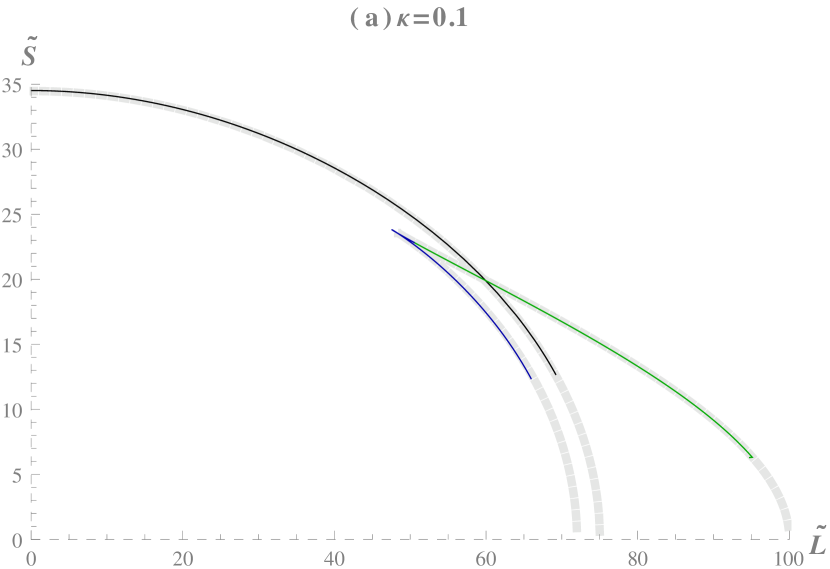
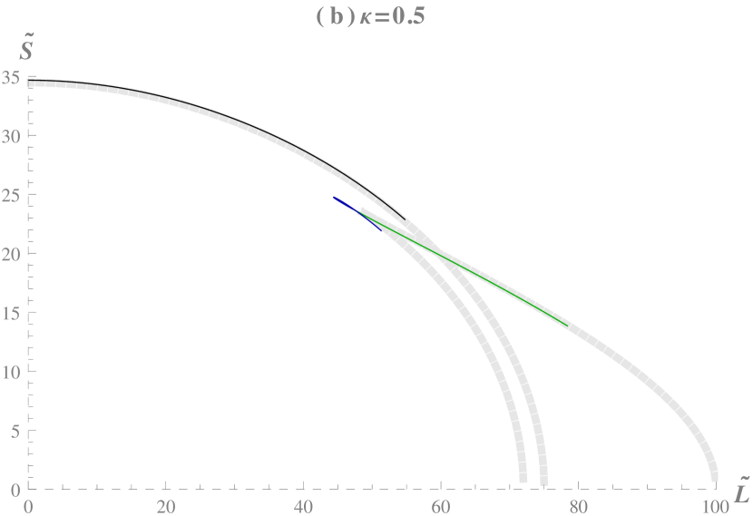
Figure 2: Phase diagram for the rotating ball and ring configurations for $\tilde{E}=40$. The blue line refers to the fat ring while the green line refers to the thin ring.

The main qualitative difference that we find here, as compared to Lahiri:2007ae , is that neither the spinning ball nor the rings reach zero entropy. This is because, at a given energy $\tilde{E}$, there is an upper bound for the velocity at the outer surface $v_{+}$, which lies below $1$, for non-zero $\kappa$. This upper bound on velocity is the point, where the curves terminate, while the curves for $\kappa=0$ continue to zero entropy as $v_{+}$ approaches $1$.

This bound on $v_{+}$ arises from the fact that the temperature at the outer surface $T_{+}$, reaches the phase transition temperature $T_{c}$ at the upper bound for $v_{+}$. At higher values of $v_{+}$, even if it remains below $1$, the temperature at the surface would drop below $T_{c}$ and the configuration would cease to exist. We have demonstrated this behaviour of the surface temperature $T_{+}$, in Fig. 3.

In Fig.3, the temperature at the outer surface of the rotating ball and the fat ring have been plotted as a function of the velocity at the outer surface $v_{+}$ at fixed energy $\tilde{E}=40$. For the thin ring, the behaviour of temperature is identical to that of the fat ring. The various lines represent values of $\kappa$ ranging from $0.1$ to $0.9$, where the darkest line corresponds to $0.9$. As it is apparent from Fig.3, the value of $v_{+}$ for which the temperature dips below the dotted blue line, representing the phase transition temperature, decreases with the increase in $\kappa$.

For the rings, there is also a lower bound on $v_{+}$, below which the solutions ceases to exist. This was also present for $\kappa=0$. Also, as it is apparent from Fig. 3, the surface temperature for all the configurations remains very close to $T_{c}$. This justifies our initial assumption that, in this analysis, we have taken the value of the surface tension and surface entropy evaluated at $T_{c}$ in (73).

The important consequence of this qualitative difference is that, for sufficiently large values of $\kappa$ the phase transition between the ball and the ring configurations may disappear. As we can see from Fig.2, such a phase transition does not exist for $\kappa=0.5$. The critical value of $\kappa$ at which this phase transition ceases to exist is approximately $0.33\approx 1/3$. Thus, we see that the temperature dependence of the surface tension can crucially affect the existence of the phase transitions between fluid configurations. In the dual gravity picture, this would have important consequence for the phase transition between black holes of different horizon topologies. This calls for a future investigation, along the lines of Aharony:2005bm from the gravity side to ascertain the value of $\kappa$.

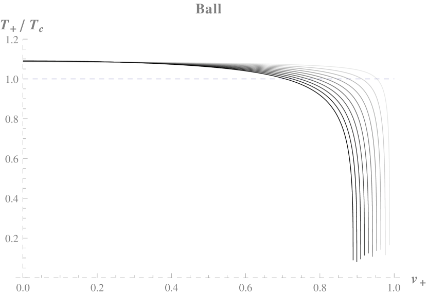
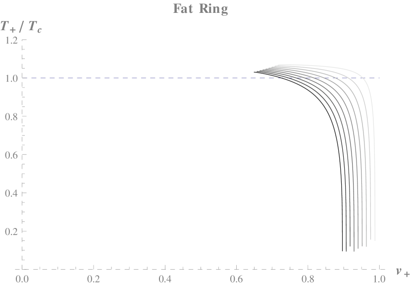
Figure 3: Temperature at the outer surface of the rotating ball and the fat ring as a function of the velocity at the outer surface $v_{+}$, at fixed energy $\tilde{E}=40$. The various lines represent values of $\kappa$, ranging from $0.1$ to $0.9$, the darkest line corresponding to $0.9$.

Finally, we would like to observe that the parameters determining the validity of our analysis are the same as in Lahiri:2007ae . The first of such parameters is given by the change in the fluid temperature over the scale of the mean free path $\Delta u\equiv\tilde{\omega}v_{+}/(1-v_{+}^{2})$, which must be small for the fluid approximation to be valid. The other parameter is $v_{+}/\tilde{\omega}$ for the ball and $\{v_{-},v_{+}-v_{-}\}/\tilde{\omega}$ for the rings, which must be large for $\delta(f)$ to be well approximated by the Dirac delta. These parameters have a $\kappa$ dependence through $\tilde{\omega}$ for a fixed value of energy. Both these parameters are not significantly affected by the value of $\kappa$ (for the values of it that we have used), in the range of parameters that we consider. Therefore, we expect the validity of our result to be as good as that in Lahiri:2007ae .

5 Discussions

In this paper, after performing a systematic analysis of the nature of surface transport in relativistic fluids, we were able to significantly constrain the structural form of the fluid equations at the surface. We have focused on some particular cases during our analysis, namely perfect fluids in arbitrary dimensions and the next to leading order corrections to 3+1 dimensional relativistic normal fluids.

Although we have a specific set up at the back of our minds, as indicated in §1, our construction may be useful in more general settings, like when boundaries between different fluid phases are present. Since we do not use any particular form for the distributions $\theta(f)$ and $\delta(f)$, they can be suitably chosen to model a wide variety of situations. In order to serve a more general purpose, it may be particularly useful to study the non-relativistic surface effects. This may be achieved by taking a non-relativistic limit of our set up following Banerjee:2015hra ; Banerjee:2015uta ; Banerjee:2014mka .

There are some immediate extensions of our work that are worth investigating. For instance, it would be very interesting to work out the next to leading order surface effects in superfluids. Due to the interplay between the vector which is normal to the surface, and the superfluid velocity, there may be a very rich, but yet unexplored surface transport properties in this case. In fact, while analyzing the zeroth order superfluids in §2.2, we noticed a new term, in the modified Young-Laplace equation (45), which has not been widely considered in the literature.

It would be very interesting to understand the implication of this term on the thermodynamics of finite lumps of superfluids. This may be accomplished by undertaking an analysis of various possible superfluid configurations along the lines discussed in §4. In fact, such an analysis may also provide direct hints towards the existence of hairy black-rings or hairy black holes with other exotic horizon topologies in Scherk-Schwarz compactified $AdS$ spacetimes via the AdS/CFT correspondence.

In section §4, we have analyzed the effects of temperature dependence of surface tension on phase diagram of some simple fluid configurations. We found that this effect can be very significant, especially while drawing conclusions about the existence of a phase transition between the ball and ring type configurations. Since, we have considered our sample system to be the same as in Lahiri:2007ae , our observation may have direct relevance for the existence of phase transition between spinning black holes and black-rings in Scherk-Schwarz compactified $AdS_{5}$. In particular, if the surface tension for these configurations scales as the inverse of temperature, then our analysis suggests that the existence of such a phase transition cannot be reliably predicted by a fluid dynamical analysis. This observation calls for generalization of Aharony:2005bm , to deduce the exact dependence of surface tension on temperature.

Another interesting extension of our work is the possible generalization to embedded fluids with surfaces of higher co-dimension and its application to the description of asymptotically flat and AdS black holes. As it is well known, both Myers-Perry black holes and the higher-dimensional Kerr-AdS black holes admit ultraspinning regimes Emparan:2003sy ; Armas:2010hz . Moreover, it was shown in Emparan:2009vd ; Armas:2010hz that these regimes can be described by a rotating fluid disc with a boundary, where the fluid is moving at the speed of light. These analytic solutions, therefore, could allow us to extract some of the new surface transport coefficients that we have found in this work and hence study the physical and stability properties of these black holes using the description of fluid dynamics with surfaces.

We would like point out one curious feature related to anomaly induced transport properties (see Jensen:2012kj ; Jensen:2013kka ; Jensen:2013rga for the most recent discussions on this). In our constructions here, we have treated the bulk of the fluid by multiplying the partition function of space filling fluids with a $\theta(f)$ function. This procedure was justified (see §1) by noting that $\theta(f)$ denoted the change in the bulk transport coefficients at or near the surface. Since the usual transport coefficients are macroscopic parameters, representing the microscopic UV theory only in an effective way, this procedure of introducing the $\theta(f)$ function is perfectly well-defined. However, there may exist certain terms in the partition function whose coefficients must be a constant as a consequence of gauge invariance Banerjee:2012iz . The terms representing transport due to anomalies (for instance the term $\mathcal{W}_{\text{anom}}$ in Banerjee:2012iz ), also falls within a similar category, since their form is fixed by the criterion that they reproduce the right anomaly coefficient locally everywhere in spacetime, including at the surface of the fluid. Such an anomaly coefficient is not an effective macroscopic parameter but a parameter of the microscopic theory. Therefore, those terms cannot be straightforwardly handled in an effective way by multiplying the, with $\theta(f)$. We postpone further analysis of these terms, in the context of fluid surfaces, to future work.

It would be interesting to see how the transport coefficients discussed in this paper fit into the classification of Haehl:2015pja ; Haehl:2014zda . Further, recently there has been significant progress in formulating dissipative fluid dynamics in terms of an action Crossley:2015evo ; Haehl:2015uoc . It would be very interesting to understand how the presence of surfaces generalizes these constructions. In fact, it would be particularly interesting to understand the time evolution of fluid surfaces, involving dissipation. If we are able to incorporate time dependence, in a controlled fashion within our set up, it may have some relevance to situations concerning dynamical formation of surfaces, in the interface of two phases, which are described by the Cahn-Hilliard equations 1958JChPh..28..258C .

Appendix A Frame transformation in the bulk

In this appendix, we shall perform a frame transformation from the Landau-frame in the bulk of the fluid, to the orthogonal-Landau-frame which was defined in §1.1.2.

In the presence of the surface at $f(x)=0$, we can choose our coordinates so that one of the spatial coordinates vanishes at the surface. Let us refer to such a coordinate by $f$. For sufficiently well behaved spacetimes, the constant $f$ surfaces would foliate the entire spacetime, including the bulk of the fluid. Every point on the constant $f$ surfaces would admit a well defined, outward pointing normal vector, which we refer to as $n_{\mu}$. This provides us with an extension of the normal vector on the surface throughout the spacetime.

As discussed in §1.1.2, instead of imposing the Landau-frame condition

$$u^{\mu}T_{\mu\nu}=-\mathcal{E}u_{\nu}$$ (84)

in the bulk, we make a slightly different frame choice, which is given by

$$\mathcal{H}^{\alpha\nu}\tilde{u}^{\mu}T_{\mu\nu}=-\mathcal{E}\tilde{u}^{\alpha},~{}~{}\tilde{u}\cdot n=0$$ (85)

to all orders, everywhere in the bulk of the fluid. Here $\mathcal{H}_{\mu\nu}=\mathcal{G}_{\mu\nu}-n_{\mu}n_{\nu}$, is the projector orthogonal $n_{\mu}$, which is defined throughout the bulk of the fluid. It possible to impose this condition everywhere in the bulk, since we now have a definition of $n_{\mu}$ extended throughout the bulk of the fluid. This immediately ensures that the fluid velocity is orthogonal to the normal vector at the surface of the fluid, where $n_{\mu}$ is unambiguously defined. This frame transformation may be achieved by simply redefining

$$\tilde{u}^{\mu}=u^{\mu}-n^{\mu}\left(u\cdot n\right)$$ (86)

Now, at the leading order, for stationary configurations, the fluid velocity can be oriented along the time-like killing vector, preserving the Landau-frame condition. Since, the surface has a trivial time evolution for stationarity configurations, this immediately implies $n\cdot u^{(0)}$ must be zero. This is no longer true at higher orders and we need to perform a frame transformation by higher derivative terms in order to achieve (85).

In the partition function construction presented in Banerjee:2012iz , the fluid velocity and temperature in the bulk, are solved in terms of the background fields. The first non-trivial corrections to the fluid velocity occurs at the second order in derivatives. This implies that we have to perform a frame transformations with second order terms, and the transformation should have a form like (86). In fact, the exact form of the required transformation can be read off from the second order corrections to the fluid velocity in Banerjee:2012iz

$$u^{\mu}=\tilde{u}^{\mu}+n^{\mu}\left(\left(\tilde{v}_{1}~{}\mathfrak{a}_{\alpha}\omega^{\alpha\nu}+\tilde{v}_{2}~{}P^{\nu}_{\alpha}\nabla_{\beta}\omega^{\beta\alpha}\right)n_{\nu}\right)+\dots,$$ (87)

where $P_{\mu\nu}=\mathcal{G}_{\mu\nu}+u_{\mu}u_{\nu}$, is the projector orthogonal to the fluid velocity and the ellipsis denote the higher order order corrections that may be necessary to keep (85) intact. We should take the coefficients $\tilde{v}_{1}$ and $\tilde{v}_{2}$ to be the same as the ones appearing in the second order velocity corrections, worked out in Banerjee:2012iz .

This frame transformations directly impacts the form of the second order stress tensor. In the Landau-frame the second order bulk stress tensor was given by (59), and is now modified to

$$\begin{split}T_{\mu\nu}=&T\left(\ \kappa_{1}~{}\tilde{R}_{\langle\mu\nu\rangle}+\kappa_{2}~{}K_{\langle\mu\nu\rangle}+\lambda_{3}\ \omega_{\langle\mu}^{\,\,\alpha}\omega_{\alpha\nu\rangle}+\lambda_{4}\ \mathfrak{a}_{\langle\mu}\mathfrak{a}_{\nu\rangle}+P_{\mu\nu}(\zeta_{2}\tilde{R}+\zeta_{3}\tilde{R}_{\alpha\beta}u^{\alpha}u^{\beta}+\xi_{3}\omega^{2}+\xi_{4}\mathfrak{a}^{2})\ \right)~{}~{}\\ &+\left(\tilde{u}_{(\mu}n_{\nu)}\left(v_{1}~{}\mathfrak{a}_{\alpha}\omega^{\alpha\rho}n_{\rho}+v_{2}~{}P^{\rho}_{\alpha}\nabla_{\beta}\omega^{\beta\alpha}n_{\rho}\right)\right)~{}~{}.\end{split}$$ (88)

Here $v_{m}=2(\mathcal{E}+P)\tilde{v}_{m}$. All the second order fluid quantities in (88) are to be expressed in terms of the transformed velocity $\tilde{u}_{\mu}$, and the vector field $n_{\mu}$ is the extension of the normal vector at the surface throughout the bulk, as explained above.

Now, we know from the partition function analysis that there are only 3 independent bulk transport coefficients and therefore $v_{1}$ and $v_{2}$ must be related to the rest of the transport coefficients, through two new relations. The necessary frame transformation to ensure (85) fixes them to be

$$v_{1}=-T^{2}\partial_{T}\left(2\kappa_{1}+\kappa_{2}-\lambda_{3}\right),v_{2}=T\left(2\kappa_{1}+\kappa_{2}-\lambda_{3}\right)~{}~{}.$$ (89)

These relations must hold in addition to the five relation between the rest of the transport coefficients in (88) as explicated in Banerjee:2012iz . The fluid velocity $\tilde{u}_{\mu}$ that will now be obtained in terms of the background data, when we compare (88) with the bulk partition function in (18), will be automatically projected orthogonal to $n_{\mu}$, which has been ensured due to the frame choice (85).

Appendix B General constraints on the stress tensor

In this appendix we discuss generic constrains and symmetries of the surface stress tensor (56). The full spacetime stress tensor, including the bulk contribution, to second order in derivatives, can be decomposed as in (11), where the surface stress tensor (56) is written in the form

$$T^{\mu\nu}_{\text{surf}}=T^{\mu\nu}_{(1)}\tilde{\delta}(f)+T^{\mu\nu\rho}_{(2)}\partial_{\rho}\tilde{\delta}(f)~{}~{}.$$ (90)

Here, the structure $T^{\mu\nu}_{(1)}$ denotes the contribution to the surface stress tensor of a monopole source of stress while $T^{\mu\nu\rho}_{(2)}$ denotes the contribution of a dipole source of stress. When applying this decomposition to (56) we easily read off

$$T^{\mu\nu\rho}_{(2)}=\left(\mathfrak{s1}_{4}\mathcal{P}^{\mu\nu}+\mathfrak{s2}_{4}u^{\mu}u^{\nu}+\mathfrak{s3}_{4}n^{\mu}n^{\nu}+\mathfrak{s4}_{4}u^{(\mu}n^{\nu)}\right)n^{\rho}+\mathfrak{v1}_{7}u^{(\mu}\mathcal{P}^{\nu)\rho}+\mathfrak{v2}_{7}n^{(\mu}\mathcal{P}^{\nu)\rho}~{}~{},$$ (91)

while $T^{\mu\nu}_{(1)}$ includes all the other surface stress tensor components.

However, we can impose additional constraints which follows from the fact that the the stress tensor (90) enjoys a symmetry, for which its components transform as (see Vasilic:2007wp for more details)

$$\delta T^{\mu\nu}_{(1)}=-\epsilon^{\mu\nu a}v_{a}~{}~{},~{}~{}\delta T^{\mu\nu\rho}_{(2)}=\epsilon^{\mu\nu a}e_{a}^{\rho}~{}~{},$$ (92)

for some coefficients $\epsilon^{\mu\nu a}$ and where we recall that we have defined $v_{a}={e_{a}}^{\rho}n^{\mu}\nabla_{\mu}n_{\rho}$. This transformation arises due to the freedom of introducing $(D-1)$ redundant delta functions in (90), so that (90) could have been written as

$$T^{\mu\nu}_{\text{surf}}=\int_{\partial\mathcal{M}}\left(T^{\mu\nu}_{(1)}\tilde{\delta}^{(D)}(f)+T^{\mu\nu\rho}_{(2)}\partial_{\rho}\tilde{\delta}^{(D)}(f)\right)~{}~{},$$ (93)

where $\tilde{\delta}^{(D)}(f)=\sqrt{\partial f.\partial f}\delta^{(1)}(x^{1})\delta^{(2)}(x^{2})...\delta^{(D-1)}(x^{D-1})\delta(f)$. Therefore, the tangential derivatives of the distribution $\tilde{\delta}(f)$ are integrated out and the coefficients $T^{\mu\nu a}_{(2)}$ can be removed Vasilic:2007wp . This implies that the terms involving $\mathfrak{v1}_{7}$ and $\mathfrak{v2}_{7}$ in (91) can be set to zero. However, the stress tensor that follows from the partition function is obtained in a fixed gauge, as far as the transformations (92) are concerned. In that case, although we do get $\mathfrak{v1}_{7}=0$, $\mathfrak{v2}_{7}$ however, is related to other transport coefficients (see (61)).

Furthermore, for a stress tensor of the form (11), there is a perturbative symmetry that allows to displace the surface located $f=0$ by a small amount $\varepsilon$ such that $f\to f+\varepsilon$. This symmetry expresses the freedom of defining the surface theory on a specific infinitely thin slice of a surface with finite thickness. Looking at Fig. 1, this means slightly displacing the dashed vertical line into another location within the distribution $\tilde{\delta}(f)$. Under this infinitesimal displacement, the form of the stress tensor (11) is unchanged but its components have varied according to

$$\delta T^{\mu\nu}=\varepsilon\left(-T^{\mu\nu}_{(0)}+n^{\rho}\partial_{\rho}T^{\mu\nu}_{(1)}\right)\tilde{\delta}(f)+\varepsilon T^{\mu\nu}_{(1)}n^{\rho}\partial_{\rho}\tilde{\delta}(f)~{}~{}.$$ (94)

From (94) we see that this transformation induces a contribution proportional to $n^{\rho}\partial_{\rho}\tilde{\delta}(f)$. If we take $T^{\mu\nu}_{(1)}$ to have the perfect fluid form at leading order, then by appropriately choosing $\varepsilon$ we could work with a surface for which either $\mathfrak{s1}_{4}$ or $\mathfrak{s2}_{4}$ vanish. However, since the transformation (94) induces a term proportional to $T^{\mu\nu}_{(0)}\tilde{\delta}(f)$, such choice of surface would require to introduce the bulk pressure $P|_{f=0}$ as an independent scalar in the surface part of the partition function. For this reason we have decided to work with the scalars $K$ and $\mathfrak{a}^{\mu}n_{\mu}$ instead.

There are structural consistency conditions on the components of the surface stress tensor (90), which, therefore, are not all independent and thus cannot be freely chosen. These consistency conditions arise due to the fact that we are working with the expansion (90) to a particular order and they can be derived by carefully analysing the conservation equation (55) to this particular order. The resulting conditions must hold in any physical situation, including time-dependent settings. One of these conditions constrains the dipole source of stress such that Vasilic:2007wp

$$n_{\mu}n_{\nu}n_{\rho}T^{\mu\nu\rho}_{(2)}=0~{}~{},$$ (95)

and also, for codimension-1 surfaces, it follows that we must have

$${e^{a}}_{\mu}n_{\nu}n_{\rho}T^{\mu\nu\rho}_{(2)}=0~{}~{},$$ (96)

which is a trivial consequence of there being no transverse two-plane on which the surface can rotate Armas:2013hsa . In turn, both conditions imply the constraints

$$\mathfrak{s3}_{4}=0~{}~{},~{}~{}\mathfrak{s4}_{4}=0~{}~{}.$$ (97)

The remaining conditions determine the normal components of the monopole source $T^{\mu\nu}_{(1)}$ in terms of the dipole source of stress $T^{\mu\nu\rho}_{(2)}$. In particular we must have that

$$\begin{split}n_{\mu}n_{\nu}T^{\mu\nu}_{(1)}&=\left(T^{ab\rho}_{(2)}K_{ab}n_{\rho}-n_{\lambda}n_{\rho}T^{\lambda\rho a}_{(2)}v_{a}\right)\\ &=\left(\mathfrak{s1}_{4}K+(\mathfrak{s1}_{4}+\mathfrak{s2}_{4})\mathfrak{a}^{\rho}n_{\rho}\right)~{}~{}.\end{split}$$ (98)

If we now evaluate the normal components of $T^{\mu\nu}_{(1)}$ in (56) we obtain

$$n_{\mu}n_{\nu}T^{\mu\nu}_{(1)}=\left(\mathfrak{s3}_{1}\mathfrak{a}^{\rho}n_{\rho}+\mathfrak{s3}_{2}K+\mathfrak{s3}_{3}\ell^{\rho}n_{\rho}\right)~{}~{},$$ (99)

which upon comparison with (98) leads to the constraints

$$\mathfrak{s3}_{1}=-(\mathfrak{s1}_{4}+\mathfrak{s2}_{4})~{}~{},~{}~{}\mathfrak{s3}_{2}=\mathfrak{s1}_{4}~{}~{},~{}~{}\mathfrak{s3}_{3}=0~{}~{}.$$ (100)

Moreover, the remaining normal components of $T^{\mu\nu}_{(0)\text{surf}}$ must respect the following condition

$$\begin{split}{e^{a}}_{\mu}n_{\nu}T^{\mu\nu}_{(1)}&=-2n_{\rho}\left(\nabla_{b}T^{ab\rho}_{(2)}+\left(T^{ac\rho}_{(2)}+T^{a\rho c}_{(2)}\right)v_{c}\right)~{}~{}\\ &=-2{\mathcal{P}^{a}}_{b}\left(\left(-T\partial_{T}\mathfrak{s1}_{4}+\mathfrak{s1}_{4}+\mathfrak{s2}_{4}\right)\mathfrak{a}^{b}+\left(\mathfrak{s1}_{4}+\frac{1}{2}\mathfrak{v2}_{7}\right)v^{b}\right)~{}~{}.\end{split}$$ (101)

Performing the same operation in (56) yields

$${e^{a}}_{\mu}n_{\nu}T^{\mu\nu}_{(1)}=\sum_{i=1}^{6}\mathfrak{v2}_{i}\mathcal{V}^{a}_{(i)}+\frac{1}{2}\sum_{i=1}^{3}\mathfrak{s4}_{i}\mathcal{S}_{(i)}u^{a}~{}~{},$$ (102)

which, again, upon comparison with (101) leads to the constraints

$$\begin{split}&\mathfrak{v2}_{i}=0~{}\forall~{}i~{}\in~{}\{2,4,5,6\}~{}~{},~{}~{}\mathfrak{v2}_{1}=2\left(T\partial_{T}\mathfrak{s1}_{4}-\mathfrak{s1}_{4}-\mathfrak{s2}_{4}\right)~{}~{},~{}~{}\mathfrak{v2}_{3}=-2\left(\mathfrak{s1}_{4}+\frac{1}{2}\mathfrak{v2}_{7}\right)~{}~{},\\ &\mathfrak{s4}_{i}=0~{}\forall~{}i~{}\in~{}\{1,2,3\}~{}~{}.\end{split}$$ (103)

As it can be quickly verified, the constraints (97),(100) and (103) are a subset of the contraints captured by the partition function analysis (61). From these considerations, we see that the only components which are left unconstrained due to stress tensor conservation are the surface components of the stress tensor $T^{ab}_{(1)}$ and the dipole source components $T^{ab\rho}_{(2)}$, also known as the bending moment. The remaining constraints in (61) in the case of relativistic fluids can be obtained by demanding positivity of the entropy current, an analysis which is carried in Appendix C.

Appendix C Entropy current constraints

In this appendix we analyze the constraints on the transport coefficients that arise from the positivity of the entropy current and show that both the partition function and the effective action capture these constraints. This can be done by analyzing the divergence of the entropy current for a membrane subjected to external forces. The equations of motion were given in (66) and(67). The fact that the equations of motion only involve $\mathbb{T}^{ab}_{\text{sur}}$, $T^{ab\rho}_{(2)}$ and $T^{\mu\nu}_{(0)}$, signifies that only these three structures are required in order specific the dynamics of the membrane. However, we need to specify what the conservation equation for the surface entropy current is. The full entropy current can be expanded analogously to the stress tensor,

$$J^{\mu}_{s}=J^{\mu}_{s(0)}\theta(f)+J^{\mu}_{s(1)}\tilde{\delta}(f)+J^{\mu\rho}_{s(2)}\partial_{\rho}\tilde{\delta}(f)+...~{}~{},$$ (104)

where the surface part, up to first order, is given by

$$J^{\mu}_{s~{}sur}=J^{\mu}_{s(1)}\tilde{\delta}(f)+J^{\mu\rho}_{s(2)}\partial_{\rho}\tilde{\delta}(f)~{}~{}.$$ (105)

For stationary configurations, we require (104) to be divergence free. In the bulk, this simply results in the bulk conservation equation $\nabla_{\mu}J^{\mu}_{s(0)}=0$ while in the surface this results in

$$\nabla_{a}\mathcal{J}^{a}_{s}=J^{\mu}_{s(0)}n_{\mu}|_{f=0}~{}~{},$$ (106)

where Armas:2013aka

$$\mathcal{J}^{a}_{s}=J^{a}_{s(1)}-{e^{a}}_{\mu}\nabla_{\rho}J^{\mu\rho}_{s(2)}-{e^{a}}_{\mu}\nabla_{a}J^{\mu b}_{s(2)}+n_{\rho}J^{b\rho}_{s(2)}{K^{a}}_{b}~{}~{}.$$ (107)

Here we have assumed that the entropy current can be obtained from the partition function/action in a similar way as a $U(1)$ charge current, in the spirit of Haehl:2015pja . From the effective action (63), the surface entropy current can be obtained via the variation Armas:2013goa ; Armas:2014rva

$$\mathcal{J}^{a}_{s}=\frac{\partial\mathcal{I}_{\text{surf}}}{\partial T}u^{a}~{}~{},$$ (108)

though, depending on the type of corrections that the bulk action receives, there may be contributions to $\mathcal{J}^{a}_{s}$ due to bulk terms. Note that we have assumed that it is always possible to write the entropy current that follows from an action in the form (108), which does not include all terms allowed by symmetry. The reason for this is that for stationary configurations we are always free to add total derivative terms to the entropy current, which are also divergence free, such that it takes the form (108). This is true for uncharged fluids up to second order in derivatives, both for the bulk entropy current and for the surface entropy current. Since (106) depends only on $\mathcal{J}^{a}_{s}$ and $J^{\mu}_{s(0)}$ it is only necessary to classify these terms in order to obtain the constraints on the fluid transport.

Before proceeding and classifying possible terms that can appear in the different relevant structures, it is important to properly define fluid frames both in the bulk and in the boundary. Because, in principle, we can be placing a completely different fluid on the surface of another bulk fluid, we should consider two fluids, each described by their own fluid variables. In this appendix, we use tilde quantities to describe the bulk fluid, which is characterized by the set of bulk variables $(\tilde{T},\tilde{u}^{\mu})$, while the surface fluid is characterized by the set of surface variables $(T,u^{\mu})$. However, in order to fully specify the system, we need to impose boundary conditions on the bulk fluid variables. These boundary conditions were described in (14) and a natural consequence of them is that

$$\tilde{u}^{\mu}\nabla_{\mu}\tilde{T}|_{f=0}=u^{a}\nabla_{a}T~{}~{}.$$ (109)

These boundary conditions are dynamical, in the sense that the evolution of $(\tilde{T},\tilde{u}^{\mu})$, described by the bulk equations to leading order

$$\tilde{u}^{\mu}\nabla_{\mu}\tilde{T}=-\tilde{s}\frac{\partial\tilde{T}}{\partial\tilde{s}}\tilde{\Theta}~{}~{},~{}~{}P^{\mu\nu}\nabla_{\nu}\tilde{T}=-\tilde{T}\tilde{\mathfrak{a}}^{\mu}~{}~{},$$ (110)

where $\tilde{\Theta}=\nabla_{\mu}\tilde{u}^{\mu}$, must be subjected to the boundary conditions (14), which are dynamically determined by the surface evolution equations to leading order

$$u^{a}\nabla_{a}T=-s\frac{\partial T}{\partial s}\Theta~{}~{},~{}~{}\mathcal{P}^{ab}\nabla_{a}T=-T{\mathfrak{a}}^{b}~{}~{}.$$ (111)

Note that (109) states that derivatives of the temperature along the fluid flows are equal in the bulk and in the surface. Derivatives of the temperature tangentially to the surface, but perpendicular to the fluid flows, are also guaranteed by (14) to be the same in both the bulk and in the surface. This can be seen by tangentially projecting the second equation in (110) and comparing it with the second equation in (111). In order to more clearly present our results, we will impose (14) from the get go while carefully keeping track of the derivatives of $\tilde{u}^{\mu}$ and $\tilde{T}$ using equations (110).

We now make a few comments regarding fluid frame transformations of the bulk and surface fluids. Frame transformations of the bulk fluid variables $(\tilde{T},\tilde{u}^{\mu})$ allows us to set the bulk stress tensor in the orthogonal-Landau frame (85), that is,

$$\mathcal{T}^{\mu\nu}_{(0)}\tilde{u}_{\mu}{\mathcal{H}^{\lambda}}_{\nu}=0~{}~{},$$ (112)

where $\mathcal{T}^{\mu\nu}_{(0)}$ are the higher derivative corrections to $T^{\mu\nu}_{(0)}$. However, due to the boundary condition (14), the restriction of such frame transformations to the surface at $f=0$ will induce a frame transformation of the surface fluid variables $(T,u^{\mu})$, if they are defined in the Landau frame. However, since we are working with stationary fluids up to second order in bulk derivatives, then such bulk frame transformations are second order in derivatives. Since the surface fluid quantities are only expanded to first order, then bulk frame transformations do not affect the surface stress tensor neither the surface entropy current. On the other hand, we can perform a first order frame transformation of the surface fluid variables $(T,u^{\mu})$ and set the surface stress tensor in the Landau frame

$$\mathbb{{T}_{(j)}}^{ab}_{\text{sur}}u_{b}=0~{}~{},$$ (113)

where again, $\mathbb{{T}_{(j)}}^{ab}_{\text{sur}}$ are the higher derivative corrections to $\mathbb{{T}}^{ab}_{\text{sur}}$.

This is not an elegant choice, in the sense that if we impose (113) for the surface stress tensor then we cannot simultaneously impose (112) for the bulk stress tensor evaluated at the surface. However, this is still a convenient choice because, as it will be explained below, the analysis of the divergence of the entropy current is insensitive to such frame transformations of the bulk stress tensor at the surface besides the fact that it reduces the number of structures appearing in the stress tensor to 4. We note, furthermore, that frame transformations do not modify the components $T^{ab\rho}_{(2)}$ of the stress tensor Armas:2013goa .

We now proceed and write the relevant terms that enter the several structures involved. We note that, since we are working in the orthogonal-Landau frame (112)-(113) and since the entropy conservation equation (106) only involves the projection of Eq. 66 along $u_{\mu}$, we find, using (88), that

$$T^{\mu\nu}_{(0)}u_{\nu}n_{\mu}|_{f=0}=-\frac{1}{2}\left(v_{1}~{}\tilde{\mathfrak{a}}_{\alpha}\tilde{\omega}^{\alpha\nu}n_{\nu}+v_{2}~{}P^{\nu}_{\alpha}\nabla_{\beta}\tilde{\omega}^{\beta\alpha}n_{\nu}\right)~{}~{}.$$ (114)

Moreover, the fact that only the contraction matters $T^{\mu\nu}_{(0)}u_{\nu}n_{\mu}|_{f=0}$ for the divergence of the entropy current implies that surface fluid frame transformations do not affect it. On the other hand, the classification of $J^{\mu}_{s(0)}$ has already been done in Bhattacharyya:2012nq . As we will see later in this section, when comparing with the partition function and effective action, the contraction $J^{\mu}_{s(0)}n_{\mu}|_{f=0}$ for stationary configurations can be written as

$$\begin{split}J^{\mu}_{s(0)}n_{\mu}|_{f=0}=&~{}\pi_{1}\Theta\mathfrak{a}^{\mu}n_{\mu}+\pi_{2}\tilde{\omega}^{\mu b}n_{\mu}\mathfrak{a}_{b}+\pi_{3}u^{a}\nabla_{a}\left(\mathfrak{a}^{\mu}n_{\mu}\right)\\ &+\pi_{4}u^{a}\mathfrak{a}^{b}{K_{ab}}+\pi_{5}\nabla_{a}\left(\tilde{\omega}^{\mu a}n_{\mu}\right)+\pi_{6}u^{a}\nabla_{a}K+\pi_{7}u^{a}\nabla_{b}{K^{b}}_{a}~{}~{}\\ &+\tilde{s}\left(v_{1}~{}\tilde{\mathfrak{a}}_{\alpha}\tilde{\omega}^{\alpha\nu}n_{\nu}+v_{2}~{}P^{\nu}_{\alpha}\nabla_{\beta}\tilde{\omega}^{\beta\alpha}n_{\nu}\right)~{}~{},\end{split}$$ (115)

where the last line above is due to the frame change (87). Here the transport coefficients $\pi_{i}$ are only functions of $T$ since we have restricted it to the surface. As the analysis of Bhattacharyya:2012nq shown, in a generic situation only 5 of the $\pi_{i}$ coefficients are independent but when stationarity is imposed, only 3 are independent Banerjee:2012iz . Furthermore, the analysis of the remaining structures has largely been done in Armas:2013goa but because of the presence of the bulk fluid and parity odd transport, we have

$$\mathbb{T}^{ab}_{\text{sur}}=\chi\mathcal{H}^{ab}+(\chi+\chi_{E})u^{a}u^{b}+\alpha_{1}K\mathcal{P}^{ab}+\alpha_{2}\mathfrak{a}^{\mu}n_{\mu}\mathcal{P}^{ab}+\alpha_{3}\ell^{\mu}n_{\mu}\mathcal{P}^{ab}+\alpha_{4}\mathcal{P}^{a}_{c}\mathcal{P}^{b}_{d}K^{cd}~{}~{},$$ (116)

$$T^{ab\rho}_{(2)}=\vartheta_{1}\mathcal{H}^{ab}n^{\rho}+\vartheta_{2}u^{a}u^{b}n^{\rho}~{}~{},$$ (117)

$$\mathcal{J}^{a}_{s}=su^{a}+\gamma_{1}Ku^{a}+\gamma_{2}\mathfrak{a}^{\mu}n_{\mu}u^{a}+\gamma_{3}\ell^{\mu}n_{\mu}u^{a}+\gamma_{4}u^{b}{K_{b}}^{a}+\gamma_{5}\tilde{\omega}^{\mu a}n_{\mu}+\gamma_{6}\epsilon^{abc}u_{b}\mathfrak{a}_{c}~{}~{}.$$ (118)

It is worthwhile keeping in mind that all the 12 surface transport coefficients are only functions of $T$. Comparing with the work in Armas:2013goa for a free membrane, we note that the terms $\alpha_{2},\alpha_{3},\vartheta_{2},\gamma_{3},\gamma_{5},\gamma_{6}$ were not present. As mentioned in Sec. B, when the bulk pressure $P$ vanishes at $f=0$, then according to (38), the scalars $K$ and $\mathfrak{a}^{\mu}n_{\mu}$ are not independent and hence we need to include $\alpha_{2}$ and $\gamma_{2}$. Consequently, we must also include the coefficient $\vartheta_{2}$. Removing it would require, as discussed in Sec. B, considering an extra term in $\mathbb{T}^{ab}_{\text{sur}}$ of the form $P|_{f=0}\mathcal{P}^{ab}$. The term $\gamma_{6}\tilde{\omega}^{\mu a}n_{\mu}$ is a consequence of the presence of the bulk degrees of freedom. For stationary configurations, it may be replaced by a term of the form $\mathcal{P}^{a}_{c}u^{b}{K_{b}}^{c}$ at the leading order; however, we must include it as a separate terms since they differ at higher orders. Finally, the coefficients $\alpha_{3},\gamma_{3},\gamma_{6}$ are well known in the context of parity odd fluids in 2+1 dimensions Jensen:2011xb and, as noticed in Jensen:2011xb , $\gamma_{3}$ and $\gamma_{6}$ are not independent. Due to the freedom of adding to (118) a total derivative term of the form $\nabla_{b}\left(\tilde{\alpha}\epsilon^{abc}u_{c}\right)$ for an arbitrary $\tilde{\alpha}$, shifting the coefficients $\gamma_{3}\to\gamma_{3}-\tilde{\alpha}$ and $\gamma_{6}\to\gamma_{6}+T\partial_{T}\tilde{\alpha}-\tilde{\alpha}$, then only the linear combination

$$\gamma_{7}=T\frac{\partial\gamma_{3}}{\partial T}+\gamma_{6}-\gamma_{3}~{}~{},$$ (119)

is invariant under this shift. The surprisingly simple form of (116) can be obtained from (56) by bringing it to the Landau frame.

Given these structures, we now impose the entropy conservation equation (106) and, using (66), obtain an expression of the following form

$$\begin{split}\nabla_{a}\mathcal{J}^{a}_{s}-J^{\mu}_{s(0)}n_{\mu}|_{f=0}=&~{}\beta_{1}\Theta K+\beta_{2}\Theta\mathfrak{a}^{\mu}n_{\mu}+\beta_{3}u^{b}\nabla_{a}{K^{a}}_{b}+\beta_{4}u^{a}\mathfrak{a}^{b}K_{ab}+\beta_{5}u^{a}\nabla_{a}K\\ &+\beta_{6}u^{a}\nabla_{a}\left(\mathfrak{a}^{\mu}n_{\mu}\right)+\beta_{7}\sigma^{ab}K_{ab}+\beta_{8}\tilde{\omega}^{\mu b}n_{\mu}\mathfrak{a}_{b}+\beta_{9}\nabla_{b}\left(\tilde{\omega}^{\mu b}n_{\mu}\right)\\ &+\beta_{10}\Theta\ell^{\mu}n_{\mu}~{}~{}.\end{split}$$ (120)

We note here that the effect of the last line of (115) is cancelled by the force term (114). Close inspection of (120) leads us to conclude that all terms involved are linear in fluid data. Since we must set the RHS of (120) to zero, according to (106), then all $\beta_{i}$ coefficients must individually vanish, i.e., we must require that $\beta_{i}=0~{},~{}\forall~{}i=1,...,10$. We can solve these constraints in terms of $\vartheta_{i},\gamma_{i}$ and the external force coefficients $\pi_{i}$ leading to

$$\begin{split}&\alpha_{4}=\gamma_{4}T~{}~{},~{}~{}\gamma_{5}=\pi_{5}~{}~{},~{}~{}\gamma_{2}T=\pi_{3}+\vartheta_{2}~{}~{},~{}~{}\gamma_{1}T=\pi_{6}T-\vartheta_{1}~{}~{},~{}~{}\gamma_{4}T=\pi_{7}T+2\vartheta_{1}~{}~{},\\ &\alpha_{1}T^{-1}=\gamma_{1}-\frac{\partial\gamma_{1}}{\partial T}s\frac{\partial T}{\partial s}~{}~{},~{}~{}2\frac{\partial\vartheta_{1}}{\partial T}=\pi_{4}+\gamma_{4}+\frac{\partial\gamma_{4}}{\partial T}T~{}~{},\\ &\frac{\partial\gamma_{5}}{\partial T}T=-\pi_{2}~{}~{},~{}~{}\alpha_{3}T^{-1}=-\gamma_{7}T\frac{\partial T}{\partial s}~{}~{},\\ &{\alpha_{2}}T^{-1}=-\pi_{1}-\left(2\frac{\partial(\vartheta_{1}-\vartheta_{2})}{T\partial T}+\frac{\partial(\gamma_{2}-\gamma_{4})}{\partial T}\right)s\frac{\partial T}{\partial s}+\gamma_{2}-2\frac{\vartheta_{2}}{T}~{}.\end{split}$$ (121)

In the case of no external forces $\pi_{i}=0$, no parity odd terms and the bulk pressure at the surface vanishing $P|_{f=0}=0$, these constraints reduce to those in Armas:2013goa , while, instead, if we have parity odd terms and require no bending corrections $\vartheta_{1}=\vartheta_{2}=0$, hence only $\alpha_{3},\gamma_{3},\gamma_{6}$ remain, then this reduces to the result of Jensen:2011xb ; Jensen:2012jh . There are a total of 10 relations in (121) relating the 6 surface transport coefficients $\alpha_{1},\alpha_{2},\alpha_{3},\alpha_{4},\vartheta_{1},\vartheta_{2}$ to the 7 external coefficients $\pi_{i}$ and the 6 entropy current coefficients $\gamma_{i}$. Of these relations, 3 of them recover relations between bulk transport coefficients which were already known from a bulk analysis Bhattacharyya:2012nq . Specifically, these are the second relation in the first line, the second relation in the second line and the first relation in the third line of (121). From the 7 remaining relations, 6 of them determine the transport coefficients $\alpha_{1},\alpha_{3},\alpha_{4}$ in terms of the transport coefficients $\vartheta_{1},\vartheta_{2}$ and the external coefficients $\pi_{i}$ while the remaining relation, namely the second relation in the third line of (121), relates the transport coefficient $\alpha_{3}$ with the linear combination $\gamma_{7}$ defined in (119) in terms of the entropy current coefficients $\gamma_{3},\gamma_{6}$ as observed in Jensen:2011xb ; Jensen:2012jh . Therefore, all surface coefficients appearing in (116)-(118) are determined in terms of the 3 transport coefficients $\alpha_{3},\vartheta_{1},\vartheta_{2}$ and 3 independent $\pi_{i}$ coefficients, as expected, since it is indeed the number of independent scalars in both the partition function (49) and the action (63).

Furthermore, from the partition function analysis, a total of 28 constraints were obtained in (61). From the analysis of Appendix B, we have obtained a total of 14 constraints from (97),(100) and (103). However, as explained in Appendix B the coefficients $\mathfrak{v1}_{7}$ and $\mathfrak{v2}_{7}$ may be removed by the transformation (92) and constitutes 2 of the 28 constraints in (61). The fact that (56) is not in the Landau gauge adds 9 extra constraints. Therefore, we have that 28-14-2-9=3, which is exactly the number of constraints that we have obtained from an entropy current analysis.

C.1 Comparison with the action and the partition function

We now compare the constraints obtained in (121) with the results obtained from the action (63) and the partition function (49). We begin by comparing (115) with the general form of the entropy current introduced in Bhattacharyya:2012nq . Using the notation of Banerjee:2012iz , the entropy current up to second order, and ignoring the first order corrections which vanish in equilibrium, can be written as

$$\begin{split}J^{\mu}_{s(0)}=&~{}\tilde{s}\tilde{u}^{\mu}+\nabla_{\nu}\left(A_{1}\left(\tilde{u}^{\mu}\nabla^{\nu}\tilde{T}-\tilde{u}^{\nu}\nabla^{\mu}\tilde{T}\right)\right)+\nabla_{\nu}\left(A_{2}\tilde{T}\tilde{\omega}^{\mu\nu}\right)+A_{3}\left(\tilde{R}^{\mu\nu}-\frac{1}{2}g^{\mu\nu}\tilde{R}\right)\tilde{u}_{\nu}\\ &+\left(A_{4}\tilde{u}^{\nu}\nabla_{\nu}\tilde{\Theta}+A_{5}\tilde{R}+A_{6}\tilde{R}^{\mu\nu}\tilde{u}_{\mu}\tilde{u}_{\nu}+B_{1}\tilde{\omega}^{2}+B_{2}\tilde{\Theta}^{2}+B_{3}\tilde{\sigma}^{2}+B_{4}\nabla_{\nu}\tilde{s}\nabla^{\nu}\tilde{s}\right)\tilde{u}^{\mu}\\ &+2B_{4}\tilde{s}\tilde{\Theta}\nabla^{\mu}\tilde{s}+\left(\tilde{\Theta}\nabla^{\mu}B_{5}-P^{\lambda\rho}\nabla_{\lambda}\tilde{u}^{\mu}\nabla_{\rho}B_{5}\right)+B_{6}\tilde{\Theta}\tilde{\mathfrak{a}}^{\mu}+B_{7}\tilde{\mathfrak{a}}_{\nu}\tilde{\sigma}^{\mu\nu}~{}~{}\\ &+\tilde{s}~{}n^{\mu}\left(v_{1}~{}\tilde{\mathfrak{a}}_{\alpha}\tilde{\omega}^{\alpha\nu}n_{\nu}+v_{2}~{}P^{\nu}_{\alpha}\nabla_{\beta}\tilde{\omega}^{\beta\alpha}n_{\nu}\right)~{}~{},\end{split}$$ (122)

where the last line above is, again, due to the frame change (87). Since we are dealing with stationary configurations for which $\Theta=\sigma^{\mu\nu}=0$ we can ignore the terms involving $A_{4},B_{2},B_{3},B_{6},B_{7}$. We now contract this bulk entropy current with $n_{\mu}$ and evaluate it at the boundary $f=0$ imposing the boundary conditions (14). We find,

$$\begin{split}J^{\mu}_{s(0)}n_{\mu}|_{f=0}=&~{}\left(A_{1}T-\frac{\partial B_{5}}{\partial T}T-\left(A_{1}+\frac{\partial A_{1}}{\partial T}T+2TB_{4}\left(\frac{\partial\tilde{s}}{\partial\tilde{T}}\right)^{2}\right)s\frac{\partial T}{\partial s}\right)\Theta\mathfrak{a}^{\mu}n_{\mu}\\ &-T\left(A_{2}+\frac{\partial A_{2}}{\partial T}T\right)\tilde{\omega}^{\mu b}n_{\mu}\mathfrak{a}_{b}+A_{1}Tu^{\mu}\nabla_{\mu}\left(\mathfrak{a}^{\mu}n_{\mu}\right)-\frac{\partial B_{5}}{\partial T}Tu^{a}\mathfrak{a}^{b}K_{ab}\\ &+A_{2}T\nabla_{a}\left(\tilde{\omega}^{\mu a}n_{\mu}\right)-A_{3}\left(u^{b}\nabla_{b}K-u^{b}\nabla_{a}{K^{a}}_{b}\right)~{}~{}\\ &+\tilde{s}\left(v_{1}~{}\tilde{\mathfrak{a}}_{\alpha}\tilde{\omega}^{\alpha\nu}n_{\nu}+v_{2}~{}P^{\nu}_{\alpha}\nabla_{\beta}\tilde{\omega}^{\beta\alpha}n_{\nu}\right)~{}~{}.\end{split}$$ (123)

Comparison of this with (115) we find read off

$$\begin{split}&\pi_{1}=A_{1}T-\frac{\partial B_{5}}{\partial T}T-(A_{1}+\frac{\partial A_{1}}{\partial T}T+2TB_{4}\left(\frac{\partial\tilde{s}}{\partial\tilde{T}}\right)^{2})s\frac{\partial T}{\partial s}~{}~{},~{}~{}\pi_{2}=-T\left(A_{2}+\frac{\partial A_{2}}{\partial T}T\right)~{}~{},\\ &\pi_{3}=A_{1}T~{}~{},~{}~{}\pi_{4}=-\frac{\partial B_{5}}{\partial T}T~{}~{},~{}~{}\pi_{5}=A_{2}T~{}~{},~{}~{}\pi_{6}=-A_{3}~{}~{},~{}~{}\pi_{7}=A_{3}~{}~{}.\end{split}$$ (124)

By obtaining the bulk stress tensor and entropy current from the action (63) and going to the orthogonal-Landau frame we obtain

$$\begin{split}&A_{1}T=-2\frac{\partial\tilde{P}_{1}}{\partial T}+2\tilde{P}_{3}~{}~{},~{}~{}A_{2}T=-\frac{2\tilde{P}_{2}}{T}~{}~{},~{}~{}A_{3}T=-2{\tilde{P}_{1}}~{}~{},\\ &B_{4}T=-\frac{2}{T}\frac{\partial\tilde{P}_{1}}{\partial T}\left(\frac{\partial\tilde{T}}{\partial\tilde{s}}\right)^{2}~{}~{},~{}\frac{\partial B_{5}}{\partial T}=-\frac{2}{T}\frac{\partial\tilde{P}_{1}}{\partial T}~{}~{}.\end{split}$$ (125)

Moreover, obtaining the surface stress tensor and surface entropy current from (63), setting it in the Landau frame and comparing it with (116) and (118) leads to

$$\begin{split}&\gamma_{1}T=-\tilde{\mathcal{B}}_{3}~{}~{},~{}~{}\gamma_{2}T=2\tilde{P}_{3}-\tilde{\mathcal{B}}_{1}-2T\frac{\partial\tilde{P}_{1}}{\partial T}~{},~{}\gamma_{3}T=2\tilde{\mathcal{B}}_{2}~{}~{},~{}~{}\gamma_{4}T=-2(\tilde{P}_{1}-\tilde{\mathcal{B}}_{3})~{}~{},~{}~{}\gamma_{5}T=-2\tilde{P}_{2}~{}~{},\\ &\gamma_{7}=2\tilde{\mathcal{B}}_{2}-\frac{\partial\tilde{\mathcal{B}}_{2}}{\partial T}T~{}~{},\vartheta_{1}=2\tilde{P}_{1}-\tilde{\mathcal{B}}_{3}~{}~{},~{}~{}\vartheta_{2}=\tilde{\mathcal{B}}_{1}~{}~{},~{}~{}\alpha_{1}=-\tilde{\mathcal{B}}_{3}+\frac{s}{T}\frac{\partial T}{\partial s}(-\tilde{\mathcal{B}}_{3}+\frac{\partial\tilde{\mathcal{B}}_{3}}{\partial T}T)~{}~{},\\ &\alpha_{2}=(\tilde{\mathcal{B}}_{1}-2T\frac{\partial\tilde{P}_{1}}{\partial T})+\frac{s}{T}\frac{\partial T}{\partial s}\left(2\tilde{P}_{3}-2\frac{\partial\tilde{P}_{1}}{\partial T}T-\frac{\partial\tilde{\mathcal{B}}_{1}}{\partial T}T-\tilde{\mathcal{B}}_{1}+2(\tilde{P}_{1}-\tilde{\mathcal{B}}_{3})\right)~{}~{},\\ &\alpha_{3}=\frac{s}{T}\frac{\partial T}{\partial s}\left(2\tilde{\mathcal{B}}_{2}-\frac{\partial\tilde{\mathcal{B}}_{2}}{\partial T}T\right)~{}~{}.\end{split}$$ (126)

One can easily check that (124)-(126) satisfy the constraints (121). We now turn into the partition function analysis of Sec. 3.3 and recast the relations (121) in terms of the transport coefficients written in (56). First, taking the stress tensor (56), we compute (116) using (68) and then set it in the Landau frame. We find the stress tensor

$$\begin{split}\mathbb{T}^{ab}_{\text{sur}}=&~{}\mathcal{P}^{ab}\left(\left(\tilde{\mathfrak{s1}}_{1}+\frac{\tilde{\mathfrak{t}}}{2}-\frac{s}{T}\frac{\partial T}{\partial s}\tilde{\mathfrak{s2}}_{1}\right)\mathfrak{a}^{\mu}n_{\mu}+\left({\mathfrak{s1}}_{2}-\frac{\tilde{\mathfrak{t}}}{2}-\frac{s}{T}\frac{\partial T}{\partial s}\tilde{\mathfrak{s2}}_{2}\right)K+\left({\mathfrak{s1}}_{3}-\frac{s}{T}\frac{\partial T}{\partial s}{\mathfrak{s2}}_{3}\right)\ell^{\mu}n_{\mu}\right)\\ &+\tilde{\mathfrak{t}}~{}\mathcal{P}^{a}_{c}\mathcal{P}^{b}_{c}K^{cd}~{}~{},\end{split}$$ (127)

where we have defined

$$\tilde{\mathfrak{s1}}_{1}={\mathfrak{s1}}_{1}-\frac{\partial\mathfrak{s1}_{4}}{\partial T}T-{\mathfrak{s1}}_{4}~{}~{},~{}~{}\tilde{\mathfrak{s2}}_{1}={\mathfrak{s2}}_{1}+\frac{\partial\mathfrak{s2}_{4}}{\partial T}T+{\mathfrak{s1}}_{4}+2{\mathfrak{s2}}_{4}~{}~{},~{}~{}\tilde{\mathfrak{s2}}_{2}={\mathfrak{s2}}_{2}-{\mathfrak{s2}}_{4}~{}~{},~{}~{}\tilde{\mathfrak{t}}={\mathfrak{t}}+2{\mathfrak{s1}}_{4}~{}~{}.$$ (128)

From here, upon comparison with (116) we read off

$$\alpha_{1}=\tilde{\mathfrak{s1}}_{1}+\frac{\tilde{\mathfrak{t}}}{2}-\frac{s}{T}\frac{\partial T}{\partial s}\tilde{\mathfrak{s2}}_{1}~{}~{},~{}~{}\alpha_{2}={\mathfrak{s1}}_{2}-\frac{\tilde{\mathfrak{t}}}{2}-\frac{s}{T}\frac{\partial T}{\partial s}\tilde{\mathfrak{s2}}_{2}~{}~{},~{}~{}\alpha_{3}={\mathfrak{s1}}_{3}-\frac{s}{T}\frac{\partial T}{\partial s}{\mathfrak{s2}}_{3}~{}~{},~{}~{}\alpha_{4}=\tilde{\mathfrak{t}}~{}~{}.$$ (129)

Furthermore, from (91) we read off the components of $T^{ab\rho}_{(2)}$,

$$\vartheta_{1}=\mathfrak{s1}_{4}~{}~{},~{}~{}\vartheta_{2}=\mathfrak{s1}_{4}+\mathfrak{s2}_{4}~{}~{}.$$ (130)

Again, we can check that (127)-(130) satisfy the constraints (121).

Appendix D Few useful relations

Under a time independent diffeomorphism $x^{\mu}\rightarrow x^{\mu}+\epsilon^{\mu}(x^{i})$ the background metric $\mathcal{G}_{\mu\nu}$ and the gauge field $\mathcal{A}_{\mu}$ transform as

$$\delta\mathcal{G}_{\mu\nu}=-(\nabla_{\mu}\epsilon_{\nu}+\nabla_{\nu}\epsilon_{\mu}),~{}\delta\mathcal{A}_{\mu}=-(\nabla_{\mu}\epsilon^{\nu}\mathcal{A}_{\nu}+\epsilon^{\nu}\nabla_{\nu}\mathcal{A}_{\mu})~{}~{}.$$ (131)

As was noted earlier an equivalent description is to consider the background fields as $\sigma,~{}a_{i},~{}g_{ij}$ for the metric and $A_{0},~{}A_{i}$ for the gauge field. Here we list out how these background fields transform under the time independent diffeomorphism written above

$$\begin{split}\delta\sigma=-\epsilon^{i}\partial_{i}\sigma~{}~{},&\delta a_{i}=-\partial_{i}\epsilon^{0}-a_{k}\partial_{i}\epsilon^{k}-\epsilon^{k}\partial_{k}a_{i}~{}~{},\delta g^{ij}=\nabla^{i}\epsilon^{j}+\nabla^{j}\epsilon^{i}~{}~{},\\ \delta A_{0}&=-\epsilon^{i}\partial_{i}A_{0}~{}~{},\delta A_{i}=-\epsilon^{k}\nabla_{k}A_{i}-\nabla_{i}\epsilon^{k}A_{k}~{}~{}.\end{split}$$ (132)

The fluid configurations discussed in section 4 were in 2+1 dimensional flat space spanned by coordinates $(t,~{}r,~{}\phi)$ with a metric

$$ds^{2}=-dt^{2}+dr^{2}+r^{2}d\phi^{2}~{}~{}.$$ (133)

We would like to change coordinates to $(t,~{}r,~{}\tilde{\phi})$, such that $t,~{}r$ remains unchanged but

$$\tilde{\phi}=\phi-\omega t~{}~{}.$$ (134)

In terms of coordinates $(t,~{}r,~{}\tilde{\phi})$, the metric in (133) becomes

$$ds^{2}=-{1\over\gamma^{2}}(dt-r^{2}\omega\gamma^{2}d\tilde{\phi})^{2}+dr^{2}+r^{2}\gamma^{2}d\tilde{\phi}^{2}~{}~{}.$$ (135)

Now comparing with (1) we obtain the corresponding background fields as given below

$$\begin{split}e^{2\sigma}={1\over\gamma^{2}}&~{}~{},~{}~{}a_{\tilde{\phi}}=-r^{2}\omega\gamma^{2}~{}~{},~{}~{}a_{r}=0~{}~{},g_{\phi\phi}=r^{2}\gamma^{2}~{}~{},~{}~{}g_{rr}=1~{}~{}.\end{split}$$ (136)

References

- (1) L. Landau and E. Lifshitz, Textbook on Theoretical Physics. VOL. 6: Fluid Mechanics, .
- (2) D. T. Son and P. Surowka, Hydrodynamics with Triangle Anomalies, Phys. Rev. Lett. 103 (2009) 191601, [arXiv:0906.5044].
- (3) J. Bhattacharya, S. Bhattacharyya, S. Minwalla, and A. Yarom, A Theory of first order dissipative superfluid dynamics, JHEP 05 (2014) 147, [arXiv:1105.3733].
- (4) S. Bhattacharyya, Constraints on the second order transport coefficients of an uncharged fluid, JHEP 07 (2012) 104, [arXiv:1201.4654].
- (5) F. M. Haehl, R. Loganayagam, and M. Rangamani, Adiabatic hydrodynamics: The eightfold way to dissipation, JHEP 05 (2015) 060, [arXiv:1502.00636].
- (6) F. M. Haehl, R. Loganayagam, and M. Rangamani, The Fluid Manifesto: Emergent symmetries, hydrodynamics, and black holes, arXiv:1510.02494.
- (7) S. Bhattacharyya, V. E. Hubeny, S. Minwalla, and M. Rangamani, Nonlinear Fluid Dynamics from Gravity, JHEP 02 (2008) 045, [arXiv:0712.2456].
- (8) N. Banerjee, J. Bhattacharya, S. Bhattacharyya, S. Dutta, R. Loganayagam, and P. Surowka, Hydrodynamics from charged black branes, JHEP 01 (2011) 094, [arXiv:0809.2596].
- (9) J. Erdmenger, M. Haack, M. Kaminski, and A. Yarom, Fluid dynamics of R-charged black holes, JHEP 01 (2009) 055, [arXiv:0809.2488].
- (10) J. Bhattacharya, S. Bhattacharyya, and S. Minwalla, Dissipative Superfluid dynamics from gravity, JHEP 04 (2011) 125, [arXiv:1101.3332].
- (11) C. P. Herzog, N. Lisker, P. Surowka, and A. Yarom, Transport in holographic superfluids, JHEP 08 (2011) 052, [arXiv:1101.3330].
- (12) O. Aharony, S. Minwalla, and T. Wiseman, Plasma-balls in large N gauge theories and localized black holes, Class. Quant. Grav. 23 (2006) 2171–2210, [hep-th/0507219].
- (13) J. Armas, How Fluids Bend: the Elastic Expansion for Higher-Dimensional Black Holes, JHEP 1309 (2013) 073, [arXiv:1304.7773].
- (14) J. Armas, (Non)-Dissipative Hydrodynamics on Embedded Surfaces, JHEP 09 (2014) 047, [arXiv:1312.0597].
- (15) J. Armas and T. Harmark, Constraints on the effective fluid theory of stationary branes, JHEP 10 (2014) 63, [arXiv:1406.7813].
- (16) W. Helfrich, Elastic Properties of Lipid Bilayers - Theory and Possible Experiments, Z. Naturforsch. C 28 (1973) 693, [arXiv:0902.3930].
- (17) P. Canham, The minimum energy of bending as a possible explanation of the biconcave shape of the human red blood cell, Journal of Theoretical Biology 26 (1970), no. 1 61 – 81.
- (18) U. Seifert, Configurations of fluid membranes and vesicles, Advances in Physics 46 (1997), no. 1 13–137.
- (19) N. Banerjee, J. Bhattacharya, S. Bhattacharyya, S. Jain, S. Minwalla, et al., Constraints on Fluid Dynamics from Equilibrium Partition Functions, JHEP 1209 (2012) 046, [arXiv:1203.3544].
- (20) K. Jensen, M. Kaminski, P. Kovtun, R. Meyer, A. Ritz, and A. Yarom, Towards hydrodynamics without an entropy current, Phys. Rev. Lett. 109 (2012) 101601, [arXiv:1203.3556].
- (21) S. Jain and T. Sharma, Anomalous charged fluids in 1+1d from equilibrium partition function, JHEP 01 (2013) 039, [arXiv:1203.5308].
- (22) N. Banerjee, S. Dutta, S. Jain, R. Loganayagam, and T. Sharma, Constraints on Anomalous Fluid in Arbitrary Dimensions, JHEP 03 (2013) 048, [arXiv:1206.6499].
- (23) S. Bhattacharyya, S. Jain, S. Minwalla, and T. Sharma, Constraints on Superfluid Hydrodynamics from Equilibrium Partition Functions, JHEP 01 (2013) 040, [arXiv:1206.6106].
- (24) S. Bhattacharyya, Entropy current and equilibrium partition function in fluid dynamics, JHEP 08 (2014) 165, [arXiv:1312.0220].
- (25) S. Bhattacharyya, Entropy Current from Partition Function: One Example, JHEP 07 (2014) 139, [arXiv:1403.7639].
- (26) K. Jensen, M. Kaminski, P. Kovtun, R. Meyer, A. Ritz, and A. Yarom, Parity-Violating Hydrodynamics in 2+1 Dimensions, JHEP 05 (2012) 102, [arXiv:1112.4498].
- (27) S. Lahiri and S. Minwalla, Plasmarings as dual black rings, JHEP 05 (2008) 001, [arXiv:0705.3404].
- (28) B. Carter, Essentials of classical brane dynamics, Int. J. Theor. Phys. 40 (2001) 2099–2130, [gr-qc/0012036].
- (29) R. Emparan, T. Harmark, V. Niarchos, and N. A. Obers, Essentials of Blackfold Dynamics, JHEP 03 (2010) 063, [arXiv:0910.1601].
- (30) J. Bhattacharya and S. Lahiri, Lumps of plasma in arbitrary dimensions, JHEP 1008 (2010) 073, [arXiv:0903.4734].
- (31) M. M. Caldarelli, O. J. C. Dias, R. Emparan, and D. Klemm, Black Holes as Lumps of Fluid, JHEP 04 (2009) 024, [arXiv:0811.2381].
- (32) L. D. Landau, Theory of the Superfluidity of Helium II, Phys. Rev. 60 (1941) 356.
- (33) L. Tisza, The Theory of Liquid Helium, Phys. Rev. 72 (1947) 838–854.
- (34) J. Bhattacharya, S. Bhattacharyya, and M. Rangamani, Non-dissipative hydrodynamics: Effective actions versus entropy current, JHEP 02 (2013) 153, [arXiv:1211.1020].
- (35) M. Vasilic and M. Vojinovic, Classical spinning branes in curved backgrounds, JHEP 07 (2007) 028, [arXiv:0707.3395].
- (36) S. Bhardwaj and J. Bhattacharya, Thermodynamics of Plasmaballs and Plasmarings in 3+1 Dimensions, JHEP 03 (2009) 101, [arXiv:0806.1897].
- (37) N. Banerjee, S. Dutta, and A. Jain, Null Fluids - A New Viewpoint of Galilean Fluids, arXiv:1509.04718.
- (38) N. Banerjee, S. Dutta, and A. Jain, Equilibrium partition function for nonrelativistic fluids, Phys. Rev. D92 (2015) 081701, [arXiv:1505.05677].
- (39) N. Banerjee, S. Dutta, A. Jain, and D. Roychowdhury, Entropy current for non-relativistic fluid, JHEP 08 (2014) 037, [arXiv:1405.5687].
- (40) R. Emparan and R. C. Myers, Instability of ultra-spinning black holes, JHEP 09 (2003) 025, [hep-th/0308056].
- (41) J. Armas and N. A. Obers, Blackfolds in (Anti)-de Sitter Backgrounds, Phys. Rev. D83 (2011) 084039, [arXiv:1012.5081].
- (42) R. Emparan, T. Harmark, V. Niarchos, and N. A. Obers, New Horizons for Black Holes and Branes, JHEP 04 (2010) 046, [arXiv:0912.2352].
- (43) K. Jensen, R. Loganayagam, and A. Yarom, Thermodynamics, gravitational anomalies and cones, JHEP 02 (2013) 088, [arXiv:1207.5824].
- (44) K. Jensen, R. Loganayagam, and A. Yarom, Anomaly inflow and thermal equilibrium, JHEP 05 (2014) 134, [arXiv:1310.7024].
- (45) K. Jensen, R. Loganayagam, and A. Yarom, Chern-Simons terms from thermal circles and anomalies, JHEP 05 (2014) 110, [arXiv:1311.2935].
- (46) F. M. Haehl, R. Loganayagam, and M. Rangamani, The eightfold way to dissipation, Phys. Rev. Lett. 114 (2015) 201601, [arXiv:1412.1090].
- (47) M. Crossley, P. Glorioso, and H. Liu, Effective field theory of dissipative fluids, arXiv:1511.03646.
- (48) F. M. Haehl, R. Loganayagam, and M. Rangamani, Topological sigma models & dissipative hydrodynamics, arXiv:1511.07809.
- (49) J. W. Cahn and J. E. Hilliard, Free Energy of a Nonuniform System. I. Interfacial Free Energy, JCP 28 (Feb., 1958) 258–267.
- (50) J. Armas, J. Gath, and N. A. Obers, Electroelasticity of Charged Black Branes, JHEP 10 (2013) 035, [arXiv:1307.0504].