Approaches to QCD phase diagram; effective models, strong-coupling lattice QCD, and compact stars

Abstract

The outline of the two lectures given in ”Dense Matter School 2015” is presented. After an overview on the relevance of the phase diagram to heavy-ion collisions and compact star phenomena, I show some basic formulae to discuss the QCD phase diagram in the mean field treatment of the Nambu-Jona-Lasinio model. Next, I introduce the strong-coupling lattice QCD, which is one of the promising methods to access the QCD phase diagram including the first order phase boundary. In the last part, I discuss the QCD phase diagram in asymmetric matter, which should be formed in compact star phenomena.

Preprint: YITP-15-127

1 Introduction

QCD phase diagram is closely related to the history of our universe and can be probed by using laboratory experiments including heavy-ion collisions. Recent developments in heavy-ion collision and compact star physics have been providing hints to understand the QCD phase diagram at finite temperature ($T$) and/or finite baryon density ($\rho_{\scriptscriptstyle B}$) as schematically shown in the left panel of Fig. 1. Heavy-ion collision data obtained at RHIC top energy ($\sqrt{s_{\scriptscriptstyle NN}}=200~{}\mathrm{GeV}$) and LHC energy (run 1, $\sqrt{s_{\scriptscriptstyle NN}}=2.76~{}\mathrm{TeV}$) imply the formation of strongly interacting matter consisting of quarks and gluons at high $T$ and almost zero $\rho_{\scriptscriptstyle B}$ [1]. The phase transition at zero $\rho_{\scriptscriptstyle B}$ is known to be a crossover from lattice QCD Monte-Carlo (LQCD-MC) simulations [2]. Crossover nature of the transition justifies the standard scenario of the homogeneous big bang nucleosynthesis. In heavy-ion collisions at lower energies, the rapidity gap between projectile and target nuclei becomes smaller. Nucleons in the projectile and target lose their energies and can get into the mid-rapidity region. Thus the nuclear stopping gives rise to the formation of hot matter at finite $\rho_{\scriptscriptstyle B}$. In the right panel of Fig. 1, we plot the density and temperature reachable in Au+Au collisions at $25A\mathrm{GeV}$ ($\sqrt{s_{\scriptscriptstyle NN}}=7.1~{}\mathrm{GeV}$) calculated in a hadron transport model, JAM [3]. In a small central box of $1~{}\mathrm{fm}^{3}$, the event averaged density may reach $9\rho_{0}$. Unfortunately, the LQCD-MC simulations suffer from the notorious sign problem, which prevents us from obtaining precise phase boundary at finite $\rho_{\scriptscriptstyle B}$ from the first principles non-perturbative calculation. Effective model calculations suggest the existence of the first order phase transition boundary at finite density [6]. It is also possible that we have the region with inhomogeneous chiral condensate instead of a sharp phase boundary [7]. If the phase transition density is not very high, we may have quark matter in the neutron star core, whose density could reach $(5-10)\rho_{0}$. Between the first order boundary (if exists) and the crossover transition, there should be a critical point (CP) [6], where the transition is the second order. Around CP, we expect large fluctuations of the order parameter and other observables which couple with the order parameter [8]. The location of CP determines the shape of the phase diagram, and CP hunting is in progress in the current beam energy scan (BES) program at RHIC [9] and will be performed in the forthcoming facilities such as FAIR, NICA, and heavy-ion beam facilities at J-PARC.

In this proceedings, I give the outline of the two lectures given in ”Dense Matter School 2015”. In the first lecture (before SQM), I explained basic idea to describe the chiral phase transition based on a mean-field treatment of a chiral effective model. In the second lecture (during SQM), I discussed how we can describe the QCD phase diagram in the strong-coupling lattice QCD. I also discussed the effects of isospin chemical potential on the phase boundary, and their implication to the compact star phenomena.

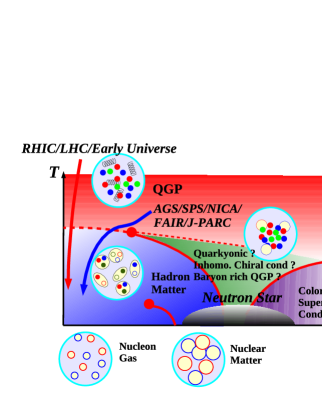
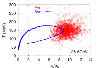
Figure 1: Left: Schematic QCD phase diagram [4]. Right: Temperature and density in 25 AGeV Au+Au collisions [5].

2 QCD phase diagram in chiral effective models

The QCD phase transition involves chiral and deconfinement transitions, and LQCD-MC results show that two transitions takes place at similar temperatures. I here concentrate on the chiral transition.

Chiral symmetry is the symmetry of QCD with massless quarks. The QCD Lagrangian is given as

$$\mathcal{L}_{\mathrm{QCD}}= \bar{q}(i\gamma^{\mu}D_{\mu}-m)q-\frac{1}{2}\mathrm{tr}F^{\mu\nu}F_{\mu\nu}$$

$$= \bar{q}_{L}(i\gamma^{\mu}D_{\mu})q_{L}+\bar{q}_{R}(i\gamma^{\mu}D_{\mu})q_{R}-(\bar{q}_{L}mq_{R}+\bar{q}_{R}mq_{L})-\frac{1}{2}\mathrm{tr}F^{\mu\nu}F_{\mu\nu}\ ,$$ (1)

where $q_{L,R}=(1\mp\gamma_{5})q/2$ are left- and right-handed quarks and $F_{\mu\nu}$ is the field strength tensor of gluon. When the quarks are massless ($m=0$), $\mathcal{L}_{\mathrm{QCD}}$ is invariant under independent rotation of $q_{L}$ and $q_{R}$ in the flavor space, $q_{L,R}\to q^{\prime}_{L,R}=U_{L,R}q_{L,R}$, where $U_{L,R}$ are $\mathrm{SU}(N_{f})$ matrices. In terms of hadrons, the chiral transformation mixes $\sigma=\bar{q}q$ and $\pi^{a}=\bar{q}i\gamma_{5}\tau^{a}q$. We should have a scalar meson having the same mass as pions if the vacuum is also invariant under the chiral transformation. In our world, the chiral condensate has a finite value in vacuum, $\langle{\bar{q}q}\rangle\not=0$, and the vacuum is not invariant under the chiral transformation. Thus the symmetry of the QCD action with massless quarks is spontaneously broken, $\mathrm{SU}(N_{f})_{L}\otimes\mathrm{SU}(N_{f})_{R}\otimes\mathrm{U}(1)_{B}\otimes\mathrm{SU}(N_{c})\to\mathrm{SU}(N_{f})_{V}\otimes\mathrm{U}(1)_{B}\otimes\mathrm{SU}(N_{c})$. This spontaneous breaking of chiral symmetry in addition to the explicit breaking (finite bare quark mass) gives rise to the mass difference of $\sigma$ and $\pi$ modes. At high $T$ and/or $\rho_{\scriptscriptstyle B}$, spontaneously broken chiral symmetry is restored, at least partially, i.e. the chiral transition takes place.

The chiral transition has been studied extensively by using chiral effective models such as the Nambu-Jona-Lasinio (NJL) model [10], the Quark Meson (QM) model [11], and Polyakov loop extended versions of them such as PNJL [12] and PQM [13] models. These models have chiral symmetry, and we expect that they could be obtained from QCD by integrating out high-momentum (short-range) degrees of freedom. Let us consider the NJL model Lagrangian,

$$\mathcal{L}_{\mathrm{NJL}}= \bar{q}(i\gamma^{\mu}\partial_{\mu}-m_{0}+\gamma_{0}\mu)q+\frac{G^{2}}{2\Lambda^{2}}\left[(\bar{q}q)^{2}+(\bar{q}i\gamma_{5}\bm{\tau}q)^{2}\right]\ ,$$ (2)

$$\mathcal{L}_{\mathrm{NJL}}^{(E)}= \bar{q}(-i\gamma_{\mu}\partial_{\mu}+m_{0}+i\gamma_{4}\mu)q-\frac{G^{2}}{2\Lambda^{2}}\left[(\bar{q}q)^{2}+(\bar{q}i\gamma_{5}\bm{\tau}q)^{2}\right]\ .$$ (3)

In the second line, we introduce the Euclidean action, $\mathcal{L}^{(E)}=-\mathcal{L}(t=-i\tau,\gamma^{0}=-i\gamma_{4},A^{0}=-iA_{4})$, where Euclidean coordinate and $\gamma$ matrices are $(x_{\mu})_{E}=(\tau=it,\mathbf{x})$ and $(\gamma_{\mu})_{E}=(i\gamma^{0},\bm{\gamma})$, respectively. The partition function in NJL is given as

$$\mathcal{Z}_{\mathrm{NJL}}= \int\mathcal{D}[q,\bar{q}]e^{-\int_{0}^{1/T}d\tau\int d\mathbf{x}\mathcal{L}^{(E)}_{\mathrm{NJL}}}=\int\mathcal{D}[q,\bar{q},\sigma,\bm{\pi}]e^{-\int d^{4}x\left\{\bar{q}Dq+\frac{\Lambda^{2}}{2}(\sigma^{2}+\bm{\pi}^{2})\right\}}$$

$$= \int\mathcal{D}[\sigma,\bm{\pi}]\exp\left[-S_{\mathrm{eff}}(\sigma,\bm{\pi};T)\right]\ ,$$ (4)

$$D= -i\gamma\partial+m_{0}+i\gamma_{4}\mu+G(\sigma+i\gamma_{5}\bm{\tau}\cdot\bm{\pi})\ ,$$

$$S_{\mathrm{eff}}= -\log\det D+\int d^{4}x\frac{\Lambda^{2}}{2}\left[\sigma^{2}(x)+\bm{\pi}^{2}(x)\right]\ .$$ (5)

In the second line, we have converted the four-Fermi interaction term in $\mathcal{L}^{(E)}_{\mathrm{NJL}}$ by using the Hubbard-Stratonovich transformation.

In order to calculate the partition function (or the free energy), we need to obtain the determinant of the fermion matrix $D$ under the anti-periodic boundary condition in the temporal coordinate, $q(1/T)=-q(0)$, for a given configuration of the auxiliary fields, $(\sigma(x),\bm{\pi}(x))$, and to integrate over the auxiliary fields. We here work in the mean field approximation in order to illustrate how the chiral transition occurs in a simple manner. In the mean field approximation, we replace the auxiliary fields with constant numbers, $(\sigma(x),\bm{\pi}(x))\to(\sigma,0)$, and $\sigma$ is chosen to minimize $S_{\mathrm{eff}}$. Then the Fermion matrix becomes a Dirac operator with modified mass, $D=-i\gamma\partial+i\gamma_{4}\mu+m(m=m_{0}+G\sigma)$. $D$ is diagonal in plane wave basis states, $D=-\gamma_{0}(i\omega+\mu)+\bm{\gamma}\cdot\mathbf{k}+m$, and the determinant is found to be $\mathrm{det}D=\prod_{n,\mathbf{k}}((\omega_{n}-i\mu)^{2}+E_{k}^{2})^{d_{f}/2}\ (E_{k}=\sqrt{\mathbf{k}^{2}+m^{2}})$, where $d_{f}=4N_{c}N_{f}$ is the Fermion degrees of freedom and $\omega_{n}=\pi T(2n-1)$ is the Matsubara frequency. Now the free energy density is obtained as

$$\mathcal{F}_{\mathrm{eff}}= -\frac{T}{V}\,\log\mathcal{Z}=\frac{\Lambda^{2}}{2}\sigma^{2}-\frac{T}{V}\sum_{n,\mathbf{k}}\,\log\left((\omega_{n}-i\mu)^{2}+E_{k}^{2}\right)^{d/2}$$

$$= \frac{\Lambda^{2}}{2}\sigma^{2}-d_{f}\int\frac{d^{3}k}{(2\pi)^{3}}\left[\frac{E_{k}}{2}+\frac{k^{2}}{3E_{k}}\,\frac{1}{2}\left(\frac{1}{e^{(E_{k}-\mu)/T}+1}+\frac{1}{e^{(E_{k}+\mu)/T}+1}\right)\right]$$

$$= \frac{\Lambda^{2}}{2}\sigma^{2}-\frac{d_{f}}{2}\Lambda^{4}I\left(\frac{m}{\Lambda}\right)-P^{(F)}\ ,$$ (6)

$$I(x)= \frac{1}{16\pi^{2}}\left[\sqrt{1+x^{2}}(2+x^{2})-x^{4}\log\frac{1+\sqrt{1+x^{2}}}{x}\right]\simeq\frac{1+x^{2}+\frac{x^{4}}{8}\left(1+4\log\frac{x}{2}\right)+\mathcal{O}(x^{6})}{8\pi^{2}}$$ (7)

From the first to the second line in Eq. (6), Matsubara frequency sum is performed. The first term in Eq. (6) comes from bosonization, and the second and third terms come from the Fermion determinant and show the zero point energy and thermal pressure, respectively.

The spontaneous symmetry breaking is understood from the shape of $\mathcal{F}_{\mathrm{eff}}$ as a function of $\sigma$. Let us consider the case in the chiral limit in vacuum ($m=0$, $T=0$ and $\mu=0$). We can ignore the thermal contribution $P^{(F)}$, and $\mathcal{F}_{\mathrm{eff}}$ can be written as

$$\mathcal{F}_{\mathrm{eff}}/\Lambda^{4}=-\frac{d_{f}}{16\pi^{2}}+\frac{x^{2}}{2}\left[\frac{1}{G^{2}}-\frac{1}{G_{c}^{2}}\right]+\mathcal{O}(x^{4}\log x)\quad(x=m/\Lambda,\ G_{c}^{2}=8\pi^{2}/d_{f})\ .$$ (8)

In the case $G>G_{c}$, the coefficient of $x^{2}$ is negative, the $\mathcal{F}_{\mathrm{eff}}$ minimum appears at $x\not=0$, and the chiral condensate is non-zero in vacuum as shown schematically in the left panel of Fig. 2. Thus if the interaction is strong enough, $\sigma(=-\langle\bar{q}q\rangle)$ condensates and constituent quark mass $m=G\sigma$ is generated.

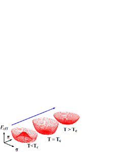
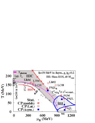
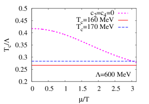
Figure 2: Left: Schematic view of the chiral phase transition. Middle: Predicted critical points and observed chemical freeze-out points [4]. Right: Tricritical point condition.

Now let us discuss the chiral transition at finite $T$ and $\mu$, where we need the mass dependence of the thermal pressure.

$$P^{(F)}/d_{f}= \frac{7}{8}\frac{\pi^{2}}{90}T^{4}+\frac{\mu^{2}}{24}T^{2}+\frac{\mu^{4}}{48\pi^{2}}-\frac{m^{2}}{16\pi^{2}}\left[\frac{\pi^{2}}{3}T^{2}+\mu^{2}\right]$$

$$- \frac{m^{4}}{32\pi^{2}}\left[\log\left(\frac{m}{\pi T}\right)-\frac{3}{4}+\gamma_{E}-H^{\nu}\left(\frac{\mu}{T}\right)\right]+\mathcal{O}(m^{6})\ ,$$ (9)

$$H^{\nu}(\nu)= \left(\frac{\nu}{\pi}\right)^{2}\sum_{l=1}^{\infty}\frac{2}{(2l-1)[(2l-1)^{2}+(\nu/\pi)^{2}]}=\sum_{k=1}^{\infty}(-1)^{k-1}\,\left(\frac{\nu}{\pi}\right)^{2k}\,\left(2-\frac{1}{2^{2k}}\right)\zeta(2k+1)\ ,$$ (10)

where $\gamma_{E}=0.5772156649\cdots$ is the Euler’s constant. The first three terms in Eq. (9) are the massless quark contributions (Stefan-Boltzmann law), and other terms show mass dependence of the pressure [15]. We again consider the chiral limit ($m_{0}=0$), then we can expand $\mathcal{F}_{\mathrm{eff}}$ in the Taylor series of $m$ as

$$\mathcal{F}_{\mathrm{eff}}(m;T,\mu)= \mathcal{F}_{\mathrm{eff}}(0;T,\mu)+\frac{c_{2}(T,\mu)}{2}\,m^{2}+\frac{c_{4}(T,\mu)}{24}\,m^{4}+\mathcal{O}(m^{6})\ ,$$ (11)

$$c_{2}(T,\mu)= \frac{d_{f}}{24}\left[T^{2}+\frac{3}{\pi^{2}}\mu^{2}-T_{c}^{2}\right]\quad\left(T_{c}^{2}=\frac{3\Lambda^{2}}{\pi^{2}}\left[1-\frac{G_{c}^{2}}{G^{2}}\right]\right)\ ,$$ (12)

$$c_{4}(T,\mu)= \frac{3d_{f}}{4\pi^{2}}\left[\gamma_{\mathrm{E}}-1-\log\left(\frac{\pi T}{2\Lambda}\right)-H^{\nu}\left(\frac{\mu}{T}\right)\right]\ .$$ (13)

We assume that the interaction is strong enough and chiral symmetry is spontaneously broken in vacuum, then $T_{c}^{2}>0$. At $\mu=0$, $c_{2}$ changes its sign at $T=T_{c}$, then the chiral restored state ($m=G\sigma=0$) is realized in equilibrium at $T>T_{c}$. This chiral transition should occur at $T<\sqrt{3}\Lambda/\pi$, which is less than the cutoff.

The second order phase boundary is given by the condition $c_{2}(T,\mu)=0$ provided that $c_{4}>0$, and is found to be $T^{2}+3\mu^{2}/\pi^{2}=T_{c}^{2}$. If this boundary reaches the $\mu$ axis, the critical baryon chemical potential is evaluated to be $N_{c}\mu_{c}=\pi N_{c}T_{c}/\sqrt{3}$, which amounts to be around the nucleon mass $N_{c}\mu_{c}\simeq 925~{}\mathrm{MeV}$ for $T_{c}\sim 170~{}\mathrm{MeV}$. This elliptically shaped phase boundary roughly explains the chemical freeze-out points probed in heavy-ion collisions, as shown in the middle panel of Fig. 2.

The second order boundary may be terminated by the tricritical point (TCP), where $c_{2}=0$ and $c_{4}=0$ is simultaneously satisfied. For the free energy density in Eq. (9), the TCP condition is expressed as

$$\frac{T_{c}}{\Lambda}=\frac{2\sqrt{1+3\nu^{2}/\pi^{2}}}{\pi}\,e^{\gamma_{E}-1-H^{\nu}(\nu)}\quad(\nu=\mu/T)\ .$$ (14)

In the right panel of Fig. 2, dotted line shows the right hand side of Eq. (14), and solid and dashed lines show $T_{c}/\Lambda$ values with $\Lambda=600~{}\mathrm{MeV}$ for $T_{c}=160~{}\mathrm{MeV}$ and $170~{}\mathrm{MeV}$, respectively. For $T_{c}=170~{}\mathrm{MeV}$, the TCP condition is satisfied around the conversion radius of the high-temperature expansion, $|\mu/T|=\pi$.

When the quark mass is finite, the transition at small $\mu$ becomes the crossover, and TCP becomes CP if the first order boundary exists. The location of CP is sensitive to the details of the model. The NJL model in the present simple treatment predicts a large $\mu/T$ value of TCP, $\mu/T\gtrsim\pi$, as discussed above. When the confinement and/or the 8-Fermi interaction effects are taken into account [16], CP temperature increases. Some lattice QCD calculations predict $T_{\mathrm{CP}}$ similar to $T_{c}(\mu=0)$. We need experimental data on CP and the first order phase transition, and/or some breakthrough in lattice QCD at finite density in order to pin down the location of CP and to understand the structure of the QCD phase diagram.

3 QCD phase diagram in strong-coupling lattice QCD

The lattice QCD Monte-Carlo (LQCD-MC) simulations is the non-perturbative and first-principles method of QCD, and have been applied to various observables such as hadron masses, hadron-hadron interactions, and QCD thermodynamics at $\mu=0$. At finite density, however, the fermion determinant becomes complex and it becomes difficult to perform precise calculation at large $\mu$. There are many methods proposed so far in order to avoid the sign problem. The strong-coupling lattice QCD is one of the promising methods.

In this section, I briefly introduce the basic idea of the lattice QCD and the sign problem. Next, I explain the strong-coupling lattice QCD.

3.1 Lattice QCD

We consider here a lattice QCD action for color $\mathrm{SU}(N_{c})$ with one species of unrooted staggered fermion in the $d(=3)+1$ dimensional Euclidean spacetime with $N_{\tau}$ temporal and $L$ spatial lattice sizes.

$$S_{\mathrm{LQCD}}= \bar{\chi}D\chi+S_{G}$$ (15)

$$= \frac{1}{2}\sum_{x}\left[\bar{\chi}_{x}U_{0}(x)\,e^{\mu}\chi_{x+\hat{0}}-\bar{\chi}_{x+\hat{0}}U_{0}^{\dagger}(x)\,e^{-\mu}\chi_{x}\right]$$

$$+ \frac{1}{2}\sum_{x,j}\eta_{j}(x)\left[\bar{\chi}_{x}U_{j}(x)\,e^{\mu}\chi_{x+\hat{j}}-\bar{\chi}_{x+\hat{j}}U_{j}^{\dagger}(x)\,e^{-\mu}\chi_{x}\right]+m_{0}\sum_{x}\bar{\chi}_{x}\chi_{x}$$

$$+ \frac{2N_{c}}{g^{2}}\sum_{\mathrm{plaq.}}\left[1-\frac{1}{N_{c}}\mathrm{Re}\,\mathrm{tr}\,U_{\mu\nu}(x)\right]\ .$$ (16)

Spacetime is discretized on the lattice, $(\tau,x,y,z)=(ai_{\tau},ai_{x},ai_{y},ai_{z})$, where $a$ is the lattice spacing and $i_{\mu}$ is an integer, $1\leq i_{\tau}\leq N_{\tau}$ and $1\leq i_{j}\leq L\ (j=1,2,3)$. In this proceedings, we adopt the lattice unit, $a=1$. Quarks are represented as anti-commuting Grassmann numbers on the lattice sites, $\chi_{x}^{a}$ (color index $a$ is suppressed in Eq. (16)). Since the square of a Grassmann number is zero, we just need to define $\int d\chi=0$ and $\int\chi d\chi=1$ to evaluate the path integral; the former is an anti-commuting constant which should be zero, and the latter is a commuting constant which can be defined as unity. Using these definitions, we find $\int\exp(\bar{\chi}A\chi)d\bar{\chi}d\chi=\det A$. The link variable $U_{\mu}(x)=P\exp\left[ig\int_{x}^{x+\hat{\mu}}dxA_{\mu}(x)\right]$ is an $N_{c}\times N_{c}$ matrix function of the gluon field and defined on a link $(x,x+\hat{\mu})$. The gauge transformation of the quark and link variables are given as $\chi_{x}\to V_{x}\chi_{x}$, $\bar{\chi}_{x}\to\bar{\chi}_{x}V_{x}$, and $U_{\mu}(x)\to V_{x}U_{\mu}(x)V_{x+\hat{\mu}}$. Then the combination $\bar{\chi}_{x}U_{\mu}(x)\chi_{x+\hat{\mu}}$ is gauge invariant. The staggered factor $\eta_{j}(x)=(-1)^{x_{0}+\cdots+x_{j-1}}$ represents $\gamma_{j}$ for staggered fermions, then the first two lines in Eq. (16) leads to the quark action in the continuum QCD. The trace of the plaquette $U_{\mu\nu}(x)=U_{\mu}(x)U_{\nu}(x+\hat{\mu})U_{\mu}^{\dagger}(x+\hat{\mu}+\hat{\nu})U_{\nu}^{\dagger}(x+\hat{\nu})$ is also gauge invariant. The loop integral $\oint dxA$ appears in the exponent in $U_{\mu\nu}$ and generates the rotation $F_{\mu\nu}$, as deduced from the Stokes theorem in the $\mathrm{U}(1)$ gauge case.

The partition function of lattice QCD is given as

$$\mathcal{Z}_{\mathrm{LQCD}}= \int\mathcal{D}[\chi,\bar{\chi},U_{0},U_{j}]\,e^{-\bar{\chi}D\chi-S_{G}}=\int\mathcal{D}[U_{0},U_{j}]\,\det D\,e^{-S_{G}}\ .$$ (17)

The integrand $\det U\,\exp(-S_{G})$ is regarded as a statistical weight for a configuration of link variables. The Fermion matrix $D$ has $\gamma_{5}$ Hermiticity, and its determinant is real at $\mu=0$,

$$\left[\gamma_{5}D(\mu)\gamma_{5}\right]^{\dagger}=D(-\mu^{*})\ ,\quad\left[\det D(\mu)\right]^{*}=\det\left[D(-\mu^{*})\right]\ .$$ (18)

Then it is possible to perform the Monte-Carlo integral by regarding $\det D\,\exp(-S_{G})$ as a statistical weight for a configuration of $U$ at zero $\mu$. At finite $\mu$, $\det D$ becomes a complex number, and a naïve probability interpretation fails down. There are many attempts to avoid the sign problem. Many of these methods are useful for $\mu/T<1$, while it is difficult to perform the Monte-Carlo simulation in the larger $\mu/T$ region, where we may expect the first order phase transition.

3.2 Strong-coupling lattice QCD

In the strong coupling region, it is possible to explore the phase diagram including the first phase transition boundary. The strong-coupling lattice QCD is a method based on the $1/g^{2}$ expansion of the partition function, and has a long history of study. In 1974, Wilson showed in the first work on the lattice gauge field theory that the Wilson loop follows the area law in the strong coupling limit [17],

$$\langle{W(C=L\times N_{\tau})}\rangle=\frac{1}{\mathcal{Z}}\int\mathcal{D}[U]W(C)\,e^{-S_{G}}\to N_{c}\left(\frac{1}{g^{2}N_{c}}\right)^{LN_{\tau}}\quad(g^{2}\to\infty)\ ,$$ (19)

where $LN_{\tau}$ is the area of the Wilson loop as shown in the left panel of Fig. 3. We need at least $LN_{\tau}$ plaquettes in order to kill all unpaired link variables. By using the one-link integral formula shown later in Eq. (20), each plaquette generates a factor $1/N_{c}g^{2}$ to the Wilson loop. The Wilson loop $W(C)=\tr P\exp(i\oint_{C}A_{\mu}dx_{\mu})$ is related with the potential between heavy quarks, $\langle{W(C)}\rangle=\exp(-V(L)N_{\tau})$. The area law tell us that $V(L)$ contains a linear confining potential, $V(L)=L\log(g^{2}N_{c})$. Thus color is found to be confined in the strong coupling region. This confining feature was confirmed by Creutz in the first lattice QCD Monte-Carlo simulation in 1980 [18]. The observed string tension is found to connect the strong coupling region and the weak coupling region smoothly. Strong-coupling expansion with higher order terms was performed by Münster [19], and the MC results are well reproduced.

Strong-coupling lattice QCD with quarks was first explored by Kawamoto and Smit [20]. It was shown that chiral symmetry is spontaneously broken in the strong-coupling limit [20, 21]. This idea is extended to finite $T$ and $\mu$ [22, 23, 24, 26, 27, 28, 30, 29]. The phase transition in the strong-coupling and chiral limit is found to be the second order at $\mu=0$ and the first order at $T=0$, in the mean field treatment [22, 23] and with fluctuation effects [27, 28]. Effects of plaquette terms at finite $1/g^{2}$ on the phase diagram are also studied [24, 30, 29].

3.3 Phase diagram at strong coupling

The plaquette term $S_{G}$ in the lattice QCD action Eq. (16) is proportional to $1/g^{2}$, and can be treated as perturbation in the strong coupling region. Especially, we can neglect $S_{G}$ in the strong coupling limit, then it is possible to integrate out the link integral independently. We can perform the one-link integral by using the formulae,

$$\int dUU_{ab}=0\ ,\int dUU_{ab}U^{\dagger}_{cd}=\frac{1}{N_{c}}\,\delta_{ad}\,\delta_{bc}\ ,\int dUU_{ab}U_{cd}U_{ef}=\frac{1}{N_{c}!}\,\varepsilon_{ace}\,\varepsilon_{bdf}\ ,\ldots$$ (20)

The second formula gives an effective action terms after integrating out spatial link variables,

$$S_{\mathrm{eff}}^{\mathrm{(SCL)}}= S_{F}^{(t)}-\frac{1}{4N_{c}}\sum_{x,j}M_{x}M_{x+\hat{j}}+m_{0}\sum_{x}M_{x}\quad(M_{x}=\bar{\chi}_{x}\chi_{x})\ ,$$ (21)

where $S_{F}^{(t)}$ is the temporal hopping term of quarks shown in the first term in Eq. (16). This effective action contains the nearest neighbor four-Fermi interaction. The third one-link integral formula generates six-Fermi interaction (baryon hopping term), which is in the sub-leading order in the large dimensional ($1/d$) expansion [25]. Let us consider the case with large spatial dimension, $d\gg 1$. In order to keep the four-Fermi interaction term finite at $d\to\infty$, quark field should scale as $\chi\propto d^{-1/4}$ to compensate a factor $d$ from the sum over $j$. The six-quark terms are $\mathcal{O}(d^{-1/2})$ for $N_{c}=3$, and we ignore them in the later discussion.

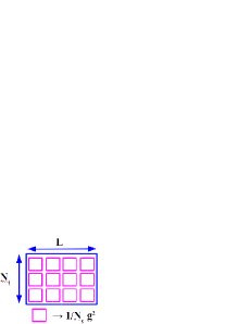
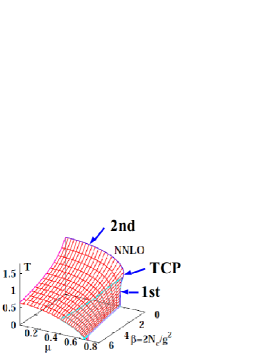
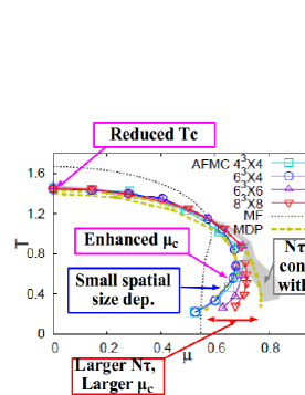
Figure 3: Left: Schematic figure of the Wilson loop. Middle: Phase diagram as a function of inverse coupling, $\beta_{g}=2N_{c}/g^{2}$ [24]. Right: Phase diagram in the strong coupling limit [28].

Once an action with four-Fermi interaction is given, there are several standard methods to solve the quantum many-body problem. One of these methods is the bosonization of the action followed by the mean field approximation and the Grassmann integral. The phase diagram in the strong coupling limit has been studied in the mean field treatment of the effective action given in Eq. (21) [23, 24]. The obtained phase diagram has similar features of that predicted in chiral effective models; the second order (crossover) transition at low $\mu$, the first order transition at large $\mu$, and the existence of TCP (CP) in (off) the chiral limit, as shown in the left panel of Fig. 3 (the $\beta=2N_{c}/g^{2}=0$ surface). This similarity of the phase diagrams owes to the symmetry of the theory. $S_{\mathrm{eff}}^{\mathrm{(SCL)}}$ in Eq. (21) [23, 24] in the chiral limit ($m_{0}=0$) is invariant under the $\mathrm{O}(2)$ chiral transformation ($\chi_{x}\to e^{i\varepsilon_{x}\alpha/2}\chi_{x}$, $\bar{\chi}_{x}\to e^{i\varepsilon_{x}\alpha/2}\bar{\chi}_{x}$), and anomaly is not realized in the strong coupling region. From the universality argument, the system with O(2) symmetry without anomaly shows the second order phase transition. This can be proxy for the system with O(4) symmetry with anomaly, as in the $N_{f}=2+1$ QCD in the chiral limit for $u$ and $d$ quarks.

The above QCD phase diagram is not satisfactory in several points; mean field approximation (no fluctuation effects), the strong coupling limit ($1/g^{2}=0$), only the leading order of the $1/d$ expansion, and one species of unrooted staggered Fermion. There are some recent progress on the fluctuation effects. One of the methods to exactly evaluate the partition function is the Monomer-Dimer-Polymer (MDP) simulation [26, 27]. We integrate out all link variables in the strong coupling limit, and we find that the partition function is represented as a sum of weights for monomer-dimer-polymer configurations. Some of the MDP configurations have negative weights, but the weight cancellation is weak. In MDP, we can also include the baryon hopping term in the sub-leading order of the $1/d$ expansion. Another method proposed so far is the auxiliary field Monte-Carlo (AFMC) method [28], which is a straightforward extension of the mean field treatment. After bosonizing the effective action, we keep the auxiliary fields as they are without putting them as constant mean fields, and integrate over the auxiliary fields using the Monte-Carlo method. We show the phase diagram obtained in these two methods in the strong coupling and chiral limit in the right panel of Fig. 3. Anisotropic lattice ($a_{\tau}\not=a_{s}$) is adopted in these calculations. Green dashed lines show the phase boundaries in MDP with $N_{\tau}=4$ and $\infty$. Solid lines with symbols show the phase boundaries in AFMC for $4^{4},6^{3}\times 4,6^{4}$ and $8^{4}$ lattices. Compared with the mean field results, fluctuation effects reduces the transition temperature at $\mu=0$, and enhance the hadron phase at large $\mu/T$. For larger $N_{\tau}$, the transition $\mu$ becomes larger. These features are common in the two methods, and the phase boundaries are found to agree with each other.

Plaquette term effects (finite $1/g^{2}$ effects) are also investigated in the mean field treatment [24]. In the middle panel of Fig. 3, we show the phase diagram as a function of $1/g^{2}$. The transition temperature decreases with increasing $1/g^{2}$ and is found to be consistent with the standard MC calculation results in the strong coupling region ($\beta_{g}=2N_{c}/g^{2}\lesssim 4$), when we take account of the $1/g^{2}$ terms and the Polyakov loop terms ($(1/g^{2})^{N_{\tau}}$). Calculations including both plaquette and fluctuation effects have been performed recently.

An interesting application of the strong-coupling lattice QCD is the net-baryon number cumulants across the phase boundary [31]. Around the phase transition, we expect large fluctuations of order parameters. The order parameter at CP is a linear combination of the chiral condensate and the baryon density [32], then larger baryon number fluctuations are expected in heavy-ion collisions at $\sqrt{s_{\scriptscriptstyle NN}}=(5-20)~{}\mathrm{GeV}$, where the formed matter is considered to go around CP. Net-baryon number cumulants

$$\chi^{(n)}=\partial^{n}(P/T^{4})/\partial(N_{c}\mu/T)^{n}=\langle(\delta B)^{n}\rangle_{c}$$ (22)

show the baryon number fluctuations, and higher-order cumulants are known to be more sensitive to the criticality [33]. Recently observed data in the beam energy scan show that the cumulant ratio $\kappa\sigma^{2}=\chi^{(4)}/\chi^{(2)}$ shows a non-monotonic behavior as a function of $\sqrt{s_{\scriptscriptstyle NN}}$, which might signal the existence of CP. Since the susceptibility ($\chi^{(2)}$) diverges at CP, it is dangerous to rely on the Taylor expansion in $\mu/T$ from $\mu=0$.

We have recently obtained the net-baryon number cumulants in the strong coupling and chiral limit. The cumulant ratio $\kappa\sigma^{2}$ shows oscillatory behavior as a function of $T$ for a given $\mu/T$, and the negative $\kappa\sigma^{2}$ region appears along the phase boundary at $\mu/T\gtrsim 0.2$. The lattice size dependence shows diverging behavior in agreement with the scaling function analysis [34]. It is important to study the finite mass effects in order to understand the observed non-monotonic behavior of $\kappa\sigma^{2}$.

4 QCD phase diagram of isospin-asymmetric matter and compact stars

Now let us turn to the compact star phenomena. In the previous sections, we have discussed the phase diagram of symmetric matter, where chemical potential is the same for all quarks. Dense matter probed in compact star phenomena, however, is not symmetric. Before the core collapse, the electron-to-baryon ratio in the iron core is around $Y_{e}\sim 0.46$, and it decreases to around $Y_{e}\sim 0.3$ as the electron capture proceeds. In neutron stars, it is further small, $Y_{e}\lesssim 0.1$. In binary neutron star mergers, $Y_{e}$ at high density is similar to that in neutron stars, while $Y_{e}$ has variety in the low density region leading to the r-process nucleosynthesis [35]. If we ignore hyperons, charge neutrality requires the same number of protons and electrons, then the proton fraction (proton-to-baryon ratio) $Y_{e}=Y_{p}=Z/(Z+N)=(0-0.46)$ in compact star phenomena. It is well known that symmetric ($N\sim Z$) and neutron-rich ($N>Z$) nuclei have different properties such as the binding energy, nuclear radius, and excitation spectra. Then we should ask ourselves. How does the QCD phase diagram evolve as a function of the proton fraction ?

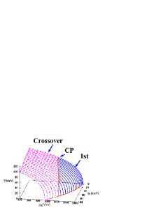
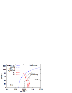
Figure 4: Left: Phase diagram as a function of isospin chemical potential [39]. Right: First order phase boundary in comparison with isospin chemical potential in neutron star matter [39].

Chiral effective model approach is again useful to explore the QCD phase diagram in asymmetric matter. We consider the Polyakov-loop extended Quark Meson (PQM) model with vector interaction,

$$\mathcal{L}_{\mathrm{PQM}}= \bar{q}\left[i\gamma^{\mu}D_{\mu}-g_{\sigma}(\sigma+i\gamma_{5}\bm{\tau}\cdot\bm{\pi})\right]q+\frac{1}{2}\partial^{\mu}\sigma\partial_{\mu}\sigma+\frac{1}{2}\partial^{\mu}\bm{\pi}\partial_{\mu}\bm{\pi}-U_{\sigma}(\sigma,\bm{\pi})-U_{\Phi}(\Phi,\bar{\Phi})$$

$$- g_{v}\bar{q}\gamma^{\mu}(\omega_{\mu}+\bm{\tau}\cdot\bm{R}_{\mu})q-\frac{1}{4}\omega_{\mu\nu}\omega^{\mu\nu}-\frac{1}{4}\bm{R}_{\mu\nu}\cdot\bm{R}^{\mu\nu}+\frac{1}{2}m_{\omega}^{2}\omega_{\mu}\omega^{\mu}+\frac{1}{2}m_{\rho}^{2}\bm{R}_{\mu}\cdot\bm{R}^{\mu}\ .$$ (23)

In addition to quarks, and $\sigma$ and $\pi$ mesons, we consider $\omega$ and $\rho$ (represented by $\bm{R}$) vector mesons. $\Phi$ and $\bar{\Phi}$ are the Polyakov and anti-Polyakov loops. The meson potential is chosen to be the sum of the zero-point energy of quarks, polynomial of $\sigma^{2}+\bm{\pi}^{2}$, and explicit breaking term $-h\sigma$. The Polyakov-loop potential is tuned to fit to the lattice results. The vector coupling of quarks are not well fixed, then we regard it is a free parameter.

In the left panel of Fig. 4, we show the QCD phase diagram in $(T,\mu_{\scriptscriptstyle B},\delta\mu)$ space, where $\delta\mu=(\mu_{d}-\mu_{u})/2=(\mu_{n}-\mu_{p})/2$ is the isospin chemical potential. We have applied the mean field approximation with an assumption that the pions do not condensate, according to the $s$-wave $\pi{N}$ repulsion argument [38]. Compared with the phase diagram of symmetric matter ($\delta\mu=0$), the transition temperature decreases with increasing $\delta\mu$. CP temperature also decreases with $\delta\mu$, and eventually CP disappears at $\delta\mu=(70-80)~{}\mathrm{MeV}$. The reduction of the transition temperature can be understood in part by using the high-temperature expansion formula in Eq. (9) and the curvature $c_{2}$ in Eq. (12) in the chiral limit. Since $u$- and $d$-quark chemical potentials are given as $\mu_{u}=\mu-\delta\mu$ and $\mu_{d}=\mu+\delta\mu$, we find $c_{2}=d_{f}/24\left[T^{2}+3(\mu^{2}+(\delta\mu)^{2})/\pi^{2}-T_{c}^{2}\right]$ for the $N_{f}=2$ NJL model in the chiral limit, and the second order phase transition temperature decreases with increasing $\delta\mu$ for given $(T,\mu=\mu_{\scriptscriptstyle B}/3)$. We expect that the effects of the vector coupling, the Polyakov loop, and finite quark mass are less sensitive to $\delta\mu$. This 3D phase diagram is similar to that obtained in the functional renormalization group (FRG) method [37], while it contradict to the effective model results with pion condensation [36].

Shrinkage of the hadron phase and the first order phase transition boundary could be relevant to compact star phenomena. First, the disappearance of the first order phase boundary at large $\delta\mu$ suggest the possibility of the crossover transition in the neutron star core. In the middle panel of Fig. 4, we show isospin chemical potential of neutron star matter in $\beta$ equilibrium as a function of baryon chemical potential calculated by using a relativistic mean field (RMF) model, TM1, in comparison with the first order phase boundary at $T=0$ in PQM with the vector-scalar coupling ratio $r=g_{v}/g_{\sigma}=0,0.2$ and $0.3$. In the cold neutron star core, $\delta\mu$ is calculated to reach around 100 MeV. When the vector coupling is not very small ($r>0.2$), the first order phase boundary disappears below $\delta\mu=80~{}\mathrm{MeV}$ and the chiral phase transition could be the crossover. If this is the case, the softening of the equation of state from the first order phase transition is weakened. This supports the crossover scenario [43] to support the $2M_{\odot}$ neutron stars [44].

Another interesting possibility is the critical point sweep during the dynamical black hole formation [40]. We consider here the numerical results in [41]; Gravitational collapse of a 40 $M_{\odot}$ star is simulated using the $\nu$ radiation 1D (spherical) hydrodynamics with the Shen EOS [42]. In failed supernovae, core collapse of massive stars directly form black holes. Temperature can reach $T\sim 90~{}\mathrm{MeV}$ at off-center by the shock heat, which is above the CP temperature of asymmetric matter in many of effective models. In the center, temperature is relatively low ($T<40~{}\mathrm{MeV}$) while the density is high ($\mu_{\scriptscriptstyle B}\sim 1300~{}\mathrm{MeV}$ just before the black hole formation). Thus there is a possibility that matter at the center goes through the first order phase transition boundary below CP, the off-center goes above CP, and some of the mass-shell hit CP. We expect large baryon number fluctuations of that mass-shell, but we have not yet found possible observational signals, unfortunately.

5 Summary

In this proceedings, I gave the outline of my two lectures in the Dense Matter 2015. We expect the existence of QCD phase transition and the critical point from chiral effective model studies. This point is discussed based on the Nambu-Jona-Lasinio model. When interaction is strong enough, chiral symmetry is spontaneously broken in vacuum. Chiral symmetry should be restored at high temperature. Density effect reduces the 4-th order coefficient in constituent quark mass which is proportional to the chiral condensate in the chiral limit. Thus we can expect the existence of the critical point and the first order transition at high density. In the lecture I also explained some technical part, such as the Matsubara sum, Hubbard-Stratonovich transformation, and high-temperature expansion. Since the first principle calculation of QCD has difficulties at finite densities, we need studies using effective models, approximate treatment of QCD, and of course, experiments.

In the second lecture, I explained other two approaches to the QCD phase diagram. The first one is the strong-coupling lattice QCD. While we have the sign problem in lattice QCD at finite $\mu$, the phase diagram study is on going using various ideas. I have shown recent results based on the strong-coupling lattice QCD. Smaller weight cancellation allow us to study phase transition at high density. Phase diagram in the strong coupling limit has been confirmed, through the agreement of MDP and AFMC results. While the strong-coupling limit is the opposite limit of the continuum limit, cumulant ratio calculation would be valuable to understand the appearance of the criticality in finite volume.

The second one is the phase diagram of asymmetric matter and compact stars. Compact stars are also good laboratories of dense matter. In neutron stars, supernovae, black hole formation, and binary neutron star mergers, we expect the formation of dense and isospin asymmetric matter. With the first order boundary (and CP) and isospin chemical potential, there are many ways of realizing phase transition in compact star phenomena.

Finally, I would like to emphasize that dense matter is ”terra incognita”, where there are many unsolved problems. In heavy-ion collisions at $\sqrt{s_{\scriptscriptstyle NN}}=(5-10)\mathrm{GeV}$, we expect formation of highest baryon density matter, whose density may exceed $5\rho_{0}$. In equilibrium, this would be above the transition density. In compact star phenomena, hydro simulations with hadronic matter EOS suggest the formation of dense matter ($(4-5)\rho_{0},\mu_{\scriptscriptstyle B}\sim 1300~{}\mathrm{MeV}$), which is above the transition density in many effective models. We need more experimental, observational, and theoretical works to explore dense matter.

The author would like to thank David Blaschke and other members in JINR for their hospitality. The author also thanks Kenta Kiuchi and Yuichiro Sekiguchi for preparing the figure for the lecture. This work is supported in part by the Grants-in-Aid for Scientific Research from JSPS (Nos. 23340067 24340054 24540271 and 15K05079 ), the Grants-in-Aid for Scientific Research on Innovative Areas from MEXT (No. 2404: 24105001, 24105008), and by the Yukawa International Program for Quark-Hadron Sciences.

References

References

- [1] Braun-Munzinger P, Magestro D, Redlich K and Stachel J 2001 Phys. Lett. B 518 41
- [2] Aoki Y et al. 2006 Nature 443 675
- [3] Nara Y, Otuka N, Ohnishi A, Niita K, Chiba S 2000 Phys. Rev. C 61 024901
- [4] Ohnishi A 2012 Prog. Thoer. Phys. Suppl. 193 1
- [5] Ohnishi A 2002 Proc. of the 2nd theory workshop on JHF nuclear physics KEK-PROC–2002-13
- [6] Asakawa M and Yazaki K 1989 Nucl. Phys. A 504 668
- [7] Nakano E and Tatsumi T 2005 Phys. Rev. D 71 114006; Nickel D 2009 Phys. Rev. D80 074025
- [8] Stephanov MA, Rajagopal K and Shuryak EV 1998 Phys. Rev. Lett. 81 4816; Asakawa M, Heinz UW and Müller B 2000 Phys. Rev. Lett. 85 2072; Jeon S and Koch V 2000 Phys. Rev. Lett. 85 2076
- [9] Adamczyk L et al. (STAR Collaboration) 2014 Phys. Rev. Lett. 112 032302
- [10] Nambu Y and Jona-Lasinio G 1961 Phys. Rev. 122 345; ibid. 124 246; Vogl U and Weise W 1991 Prog. Part. Nucl. Phys. 27 195; Klevansky SP 1992 Rev. Mod. Phys. 64 649; Hatsuda T and Kunihiro T 1994 Phys. Rept. 247 221; Buballa M 2005 Phys. Rept. 407 205
- [11] Jungnickel DU and Wetterich C 1996 Phys. Rev. D 53 5142
- [12] Fukushima K 2004 Phys. Lett. B 591 277
- [13] Schaefer BJ, Pawlowski JM and Wambach J 2007 Phys. Rev. D76 074023; Skokov V, Friman B, Nakano E, Redlich K and Schaefer BJ 2010 Phys. Rev. D 82 034029
- [14] Yagi K, Hatsuda T, Miake Y 2005 Quark-Gluon Plasma: From Big Bang to Little Bang (Cambridge, Cambridge University Press)
- [15] Kapusta JI and Gale C 2006 Finite-Temperature Field Theory: Principles and Applications (Cambridge, Cambridge University Press)
- [16] Sasaki T, Sakai Y, Kouno H and Yahiro M 2010 Phys. Rev. D 82 116004
- [17] Wilson KG 1974 Phys. Rev. D 10 2445
- [18] Creutz M 1980 Phys. Rev. D 21 2308
- [19] Munster G 1981 Nucl. Phys. B 180 23
- [20] Kawamoto N 1981 Nucl. Phys. B 190 [FS3] 617; Kawamoto N and Smit J 1981 Nucl. Phys. B 192 100
- [21] Aoki S 1984 Phys.Rev. D 30 2653
- [22] Damgaard PH, Kawamoto N and Shigemoto K 1984 Phys. Lett. B 114 152; Faldt G and Petersson B 1986 Nucl. Phys. B 265 197;
- [23] Ilgenfritz EM and Kripfganz J 1985 Z. Phys. C29 79; Bilic N, Karsch F and Redlich K 1992 Phys. Rev. D45 3228; Fukushima K 2004 Prog. Theor. Phys. Suppl. 153 204; Nishida Y 2004 Phys. Rev. D 69 094501; Kawamoto N, Miura K, Ohnishi A and Ohnuma T 2007 Phys. Rev. D75 014502
- [24] Miura K, Nakano TZ and Ohnishi A 2009 Prog. Theor. Phys. 122 1045; Miura K, Nakano TZ, Ohnishi A and Kawamoto N 2009 Phys. Rev. D 80 074034; Nakano TZ, Miura K and Ohnishi A 2010 Prog. Theor. Phys. 123 825; Nakano TZ, Miura K and Ohnishi A 2011 Phys. Rev. D 83 016014; Ohnishi A, Miura K, Nakano TZ and Kawamoto K 2009 PoS LATTICE 2009 160
- [25] Kluberg-Stern H, Morel A and Petersson B 1983 Nucl. Phys. B 215 [FS7] 527
- [26] Karsch F and Mutter KH 1989 Nucl. Phys. B 313 541
- [27] de Forcrand P and Fromm M 2010 Phys. Rev. Lett. 104 112005
- [28] Ichihara T, Ohnishi A and Nakano TZ 2014 Prog. Theor. Exp. Phys. 2014 123D02
- [29] Ichihara T and Ohnishi A 2014 PoS LATTICE2014 188 (Preprint arXiv:1503.07049 [hep-lat])
- [30] de Forcrand P, Langelage J, Philipsen O and Unger W 2014 Phys. Rev. Lett. 113 152002
- [31] Ichihara T, Morita K and Ohnishi 2015 Prog. Theor. Exp. Phys. 2015 113D01 (Preprint arXiv::1507.04527 [hep-lat])
- [32] Fujii H and Ohtani M 2004 Phys. Rev. D 70 014016
- [33] Stephanov MA 2009 Phys. Rev. Lett. 102 032301
- [34] Friman B, Karsch F, Redlich K and Skokov V 2011 Eur. Phys. J. C 71 1694
- [35] Sekiguchi Y, Kiuchi K, Kyotoku K, Shibata M 2015 Phys. Rev. D 91 064059
- [36] Sasaki T, Sakai Y, Kouno H and Yahiro M 2010 Phys. Rev. D 82 116004; Andersen JO and Kyllingstad L 2010 J. Phys. G 37 015003
- [37] Kamikado K, Strodthoff N, von Smekal L and Wambach J 2013 Phys. Lett. B 718 1044
- [38] Ohnishi A, Jido D, Sekihara T and Tsubakihara K 2009 Phys. Rev. C 80 038202
- [39] Ueda H, Nakano TZ, Ohnishi A, Ruggieri M and Sumiyoshi K 2013 Phys. Rev. D 88 074006
- [40] Ohnishi A, Ueda H, Nakano TZ, Ruggieri M, Sumiyoshi K 2011 Phys. Lett. B 704 284
- [41] Sumiyoshi K, Yamada S, Suzuki H and Chiba S 2006 Phys. Rev. Lett. 97 091101
- [42] Shen H, Toki H, Oyamatsu K and Sumiyoshi K 1998 Nucl. Phys. A 637 436; Prog. Theor. Phys. 100 1013
- [43] Masuda K, Hatsuda T and Takatsuka T 2013 Astrophys. J. 764 12; Prog. Theor. Exp. Phys. 2013 073D01
- [44] Demorest P et al. 2010 Nature 467 1081; Antoniadis J et al. 2013 Science 340 448