UWThPh-2015-34  


Ergostatting and Thermostatting at a Fixed Point

Abstract

We propose a novel type of ergostats and thermostats for molecular dynamics simulations. A general class of active particle swarm models is considered, where any specific total energy (alternatively any specific temperature) can be provided at a fixed point of the evolution of the swarm. We identify the extended system feedback force of the Nosé - Hoover thermostat with the “internal energy” variable of active Brownian motion.

1 Introduction

In this paper a novel type of ergostats and thermostats for molecular dynamics simulations is proposed, which is derived from particle swarm models. An assigned total energy or temperature can be provided at fixed points of the evolution of the swarms.

Simulations in molecular dynamics are usually performed in the microcanonical ensemble, where the number of particles, volume, and energy have constant values. In experiments, however, it is the temperature which is controlled instead of the energy. Several methods have been advanced for keeping the temperature constant in molecular dynamics simulations. Popular are deterministic thermostats like velocity rescaling [1], the Andersen thermostat [2], the Nosé–Hoover thermostat [3, 4, 5, 6, 7] and its generalizations [8, 9, 10, 11, 12], Nosé–Hoover chains [13], and the Berendsen thermostat [14]. Gauss’ principle of least constraint was utilized by Evans, Hoover and collaborators to develop isokinetic [15], as well as isoenergetic (=ergostatic) thermostats [16]. Dettmann and Morriss [17, 18] as well as Bond, Laird, and Leimkuhler [19] discovered Hamiltonian schemes for both the Nosé- Hoover and Gaussian thermostats. Another setting arises for stochastic thermostats, which includes standard Brownian (overdamped Langevin) and Langevin dynamics, as well as stochastic thermostats of Nosé–Hoover–Langevin type [20, 21] and generalizations thereof [22]. Stochastic velocity rescaling which can be considered as Berendsen thermostat plus a stochastic correction leading to canonical sampling was considered by [23, 24, 25, 26]. For further discussion on the various thermostatting schemes, we refer to the recent monographs [27, 28, 29].

Swarming - the collective, coherent, self organized motion of a large number of organisms - is one of the most familiar and widespread biological phenomena at the interface of physics and biology. Universal features of swarming have been identified and diverse physical models of swarming have been proposed (see the reviews [30, 31, 32]).

Amongst these models there is a whole class, often referred to as active [33, 34], which provides a relevant tool for simulating complex systems (see the monographs [35, 36]). The notion active refers to the property of particles to take up energy from their environment and store it as so-called internal energy. This then is followed by the generation of an out-of equilibrium state of the system and depending on the particular circumstances is implying self-propulsion, alignment, attraction or repulsion of the particles.

Recently a simple model for particle swarms was proposed [37, 38], which is the starting point for our present discussion. The model is specified by a $(2dN+1)$-dimensional system of first order differential equations for coordinates and momenta of $N$ active particles in $d$ space dimensions coupled to internal energy. Such a nonlinear system is not easily accessible with direct analytic procedures. Nonetheless, precise predictions for the system’s long time behavior can be made in the case where all particles are attracted with harmonic forces. We focus on the time evolution of macroscopic swarm variables, represented by the total kinetic energy, total potential energy, virial and - last but not least - internal energy. A closed four-dimensional system of first order differential equations for the time evolution of these macroscopic swarm variables can be obtained. In the long time limit one finds a stable equilibrium configuration with fixed non-zero total kinetic and potential energy, whereas internal energy and virial are vanishing, see Fig. 2 and Fig. 3 below. Bifurcation analysis provides us with conditions on parameters of the model for this to take place [37, 38].

It is intriguing to observe that in the equilibrium state with fixed total kinetic energy the system effectively becomes thermostatted. Thus a novel and original method of thermostatting at fixed points of the evolution of particle swarms has been obtained. The usual Nosé-Hoover dynamics [3, 4, 5, 6, 7] has no attractive fixed point, and in contrast to the Gaussian isokinetic [15] thermostat, no constraint needs to be implemented. It is in the fixed point limit of the system’s evolution that the total kinetic energy becomes conserved.

In Section 2 we shortly review active multi-particle systems. Then in Section 3 basic features of the fixed point method for thermostatting as well as the related procedure for ergostatting are outlined. In Section 4 prototype studies of the active ergostat and thermostat are given for a single particle in two-dimensional space. Harmonic multi-particle systems in Sections 5 and 6, as well as multi-particle systems with Lennard-Jones inter-particle forces in Sections 7 and 8, respectively, constitute the main body of our paper. A final discussion of our results, indicating several applications, is given in Section 9.

2 Particle swarm models

2.1 Active multi-particle systems

We consider a multi-particle system of $N$ active particles [37, 38], enumerated by the index $i$, with equal masses $m$ in $d$ space dimensions coupled to the internal energy $e$. The position and momentum vectors are $\textbf{x}_{i},\textbf{p}_{i}\in\textbf{R}^{d}$ with $i=1,\dots,N$ and the equations of motion read

$$\dot{\textbf{x}}_{i}=\frac{\partial H}{\partial\textbf{p}_{i}},$$ (1)

$$\dot{\textbf{p}}_{i}=-\left(1-d_{1}e\right)\frac{\partial H}{\partial\textbf{x}_{i}}-\left(\gamma-d_{2}e\right)m\frac{\partial H}{\partial\textbf{p}_{i}},$$ (2)

$$\dot{e}=1-c_{1}e-c_{2}k\,e-c_{3}u\,e,$$ (3)

where the total Hamiltonian $H=N\,h$ is the sum of kinetic $K=Nk$ and potential energy $U=Nu$ given by

$$H=K+U,\qquad K=\sum_{i=1}^{N}\frac{\textbf{p}_{i}^{2}}{2m},\qquad U=\sum_{i=1}^{N}U_{i}^{(ext)}+\frac{1}{2}\sum_{i,j=1}^{N}U_{ij}^{(int)}.$$ (4)

The potential energy $U$ of the swarm is composed of the external potentials $U_{i}^{(ext)}$, modeling the environment of the swarm, and of the potentials $U_{ij}^{(int)}$, describing the pairwise interactions among the particles. The swarm model is specified by the potential $U$ and a set of parameters $c_{1},c_{2},c_{3},d_{1},d_{2}$ and $\gamma.$ An active swarm model where $c_{2}=c_{3}$ is called canonical.

We note that in the fast feedback limit of internal energy a related active swarm model was studied previously [39].

2.2 Swarm dynamics for a harmonic multi-particle system

Here we study the case where all particles are attracted with harmonic forces, for simplicity no external forces are considered. The total Hamiltonian then reads

$$H=\sum_{i=1}^{N}\frac{\textbf{p}_{i}^{2}}{2m}+\sum_{i,j=1}^{N}\frac{m\,\omega_{0}^{2}}{4}\left(\textbf{x}_{i}-\textbf{x}_{j}\right)^{2}.$$ (5)

In the center of mass frame the swarm dynamics is given by

$$\dot{\textbf{x}}_{i} = \frac{\textbf{p}_{i}}{m},$$ (6)

$$\dot{\textbf{p}}_{i} = -\left(1-d_{1}e\right)N\,m\,\omega_{0}^{2}\,\textbf{x}_{i}-\left(\gamma-d_{2}e\right)\textbf{p}_{i},$$ (7)

$$\dot{e} = 1-c_{1}e-c_{2}k\,e-c_{3}u\,e.$$ (8)

The above system of coupled nonlinear differential equations is not easily accessible with direct analytic procedures. Nonetheless, predictions for the system’s long time behavior can be made by transforming to macroscopic swarm variables

$$e,\quad K=\sum_{i=1}^{N}\frac{\textbf{p}_{i}^{2}}{2m},\quad U=N\,m\,\omega_{0}^{2}\sum_{i=1}^{N}\frac{\textbf{x}_{i}^{2}}{2},\quad S=\frac{\sqrt{N}\omega_{0}}{2}\sum_{i=1}^{N}\textbf{x}_{i}\cdot\textbf{p}_{i}.$$ (9)

$K$ represents the total kinetic energy of the swarm, $U$ the total internal potential energy, $S=Ns$ denotes the virial. We also introduce the corresponding intensive quantities $k,u,s$ and recall $H=Nh=N(k+u)$. These definitions of the macroscopic swarm variables are valid in any spatial dimension $d$ of the system. The differential equations now read

$${\color[rgb]{0,0,0}\dot{k}} {\color[rgb]{0,0,0}=} {\color[rgb]{0,0,0}-\left(1-d_{1}\,{\color[rgb]{1,0,0}{\color[rgb]{0,0,0}e}}\right)2\sqrt{N}\omega_{0}s-2\left(\gamma-d_{2}\,{\color[rgb]{1,0,0}{\color[rgb]{0,0,0}e}}\right)\,k,}$$ (10)

$${\color[rgb]{0,0,0}\dot{u}} {\color[rgb]{0,0,0}=} 2\sqrt{N}\omega_{0}{\color[rgb]{0,0,0}s,}$$ (11)

$${\color[rgb]{0,0,0}\dot{s}} {\color[rgb]{0,0,0}=} {\color[rgb]{0,0,0}\sqrt{N}\omega_{0}k-\left(1-d_{1}\,{\color[rgb]{1,0,0}{\color[rgb]{0,0,0}e}}\right)\sqrt{N}\omega_{0}u-\left(\gamma-d_{2}\,{\color[rgb]{1,0,0}{\color[rgb]{0,0,0}e}}\right)\,s,}$$ (12)

$${\color[rgb]{0,0,0}{\color[rgb]{0,0,0}\dot{{\color[rgb]{1,0,0}{\color[rgb]{1,0,0}{\color[rgb]{0,0,0}e}}}}}} {\color[rgb]{0,0,0}{\color[rgb]{0,0,0}=}} 1-c_{1}e-c_{2}k\,e-c_{3}u\,e.$$ (13)

We have thus reduced the $(2dN+1)$-dimensional system $(6)-(8)$ of first order differential equations for coordinates, momenta and internal energy to a $4$-dimensional system of first order differential equations $(10)-(13)$ for the macroscopic swarm variables.

In the long time limit an equilibrium state which corresponds to amorphous swarming could be obtained by finding a stable fixed point $(k_{0},u_{0},s_{0},e_{0})$ with non-vanishing kinetic energy $k_{0}$. Bifurcation analysis provides us with conditions for the parameters $c_{1,}c_{2},c_{3},d_{1},d_{2},\gamma$ for this to take place, see [37, 38]. It is obvious that a system in a swarming equilibrium state effectively becomes thermostatted, so a novel method of thermostatting appears to be indicated.

Active swarm dynamics with its many parameters necessitates quite an involved study of the various arising phenomena. In this paper we therefore focus on simplified and more manageable time evolutions of active swarms, setting $d_{1}=c_{1}=0$.

• Within the canonical formulation where $c_{2}=c_{3}$ we will demonstrate that equilibrium states with fixed total energy may emerge in the long time limit. It is precisely this phenomenon, which defines our novel type of active ergostats. We will discuss several applications.
  
  

• Studying the related swarm dynamics with $d_{1}=c_{1}=0$ and $c_{3}=0$ we find equilibrium states with fixed kinetic energy. This defines our novel type of active thermostats. We will explore features of such a novel method of thermostatting, give its relation to the Nosé-Hoover thermostat and discuss several applications.
  

We close by reminding that also static long time limits of a swarm exist, where all particles are collapsing to a single point or freezing according to a certain pattern. This is of no concern in the present investigation of ergostats and thermostats, however.

3 Ergostats and thermostats

3.1 Nosé-Hoover thermostat

The novel type of ergostats and thermostats we are going to present reminds in some aspects of the Nosé–Hoover thermostat, which we will review now. In order to model a system of $N$ particles coupled to a thermal reservoir at temperature $T$ Nosé [4] defined an extended Hamiltonian with additional canonically conjugated degrees of freedom $s,P_{s}$ representing the heat bath; also a parameter $Q$ named Nosé mass parameter was introduced. The equations of motion in the so called Nosé - Hoover form [6] are given by

$$\dot{\textbf{x}}_{i} = \frac{\textbf{p}_{i}}{m},$$ (14)

$$\dot{\textbf{p}_{i}} = -\frac{\partial U}{\partial\mathbf{x_{i}}}-\xi\,\mathbf{p_{i}},$$ (15)

$$\dot{\xi} = \frac{1}{\tau^{2}}\,\left(\frac{k}{k_{0}}-1\right).$$ (16)

Here $\xi=\frac{P_{s}}{Q}$ acts like an extended system feedback force controlling the kinetic energy $k$. The Temperature $T$ of the system is related to the average kinetic energy $k_{0}$ by $T=\frac{2}{d}\,k_{0}$, the relaxation time $\tau$ is defined by $\tau^{2}=\frac{Q}{2Nk_{0}}$.

Nosé proved analytically that the microcanonical probability measure on the extended variable phase space reduces to a canonical probability measure on the physical variable phase space $(\mathbf{x}_{i},\mathbf{p_{i}})$. The Nosé–Hoover thermostat has been commonly used as one of the most accurate and efficient methods for constant-temperature molecular dynamics simulations.

3.2 Active ergostat and ergostatting in the fixed point

Substituting into the active multi-particle system $(1)-(3)$ the special parameter values

$$c_{1}=0,\quad c_{2}=c_{3}=\frac{1}{h_{0}\tau_{2}},\quad d_{1}=0,\quad d_{2}=\frac{1}{\left(\tau_{1}\right)^{2}},\quad\gamma=\frac{\tau_{2}}{\left(\tau_{1}\right)^{2}},$$ (17)

as well as transforming variables

$$e\rightarrow\xi=\gamma-d_{2}\,e$$ (18)

we arrive at equations of motion which are of a generalized Nosé - Hoover form

$$\dot{\textbf{x}}_{i} = \frac{\textbf{p}_{i}}{m},$$ (19)

$$\dot{\textbf{p}_{i}} = -\frac{\partial U}{\partial\mathbf{x_{i}}}-\xi\,\mathbf{p_{i}},$$ (20)

$$\dot{\xi} = \frac{1}{\left(\tau_{1}\right)^{2}}\left(\frac{h}{h_{0}}-1\right)-\frac{h}{\tau_{2}\,h_{0}}\,\xi.$$ (21)

The evolution equations may have an attractive fixed point in which the averaged total energy per particle $h=h_{0}$ becomes sharply fixed. This specific form of ergostat we would like to call the active ergostat ($AE$).

It should be remarked that for simplicity we defined the $\dot{\xi}$ equation (21) under the assumption that $h_{0},\,h>0\text{}$. For negative values of $h_{0}$ and possibly also for negative $h$ appropriate sign flips have to be added, see the discussion in section 3.2.

3.3 Active thermostat and thermostatting in the fixed point

At this place we mention an interesting variant of the above derivation, which lead to (21). For the swarm evolution $(1)-(3)$ we consider now $c_{1}=c_{3}=d_{1}=0$ and have

$$\dot{\textbf{x}}_{i}=\frac{\partial H}{\partial\textbf{p}_{i}},$$ (22)

$$\dot{\textbf{p}}_{i}=-\frac{\partial H}{\partial\textbf{x}_{i}}-\left(\gamma-d_{2}e\right)m\frac{\partial H}{\partial\textbf{p}_{i}},$$ (23)

$$\dot{e}=1-c_{2}k\,e.$$ (24)

Different from $(3)$, where the internal energy couples to the total energy, here in (24) the internal energy couples to the kinetic energy only. This kind of dynamics was introduced and explored in several applications by [34, 35]. Choosing similar parameter values as before

$$c_{2}=\frac{1}{k_{0}\tau_{2}},\quad d_{2}=\frac{1}{\left(\tau_{1}\right)^{2}},\quad\gamma=\frac{\tau_{2}}{\left(\tau_{1}\right)^{2}}$$ (25)

we again transform variables according to (18) and finally are arriving at

$$\dot{\textbf{x}}_{i} = \frac{\textbf{p}_{i}}{m},$$ (26)

$$\dot{\textbf{p}_{i}} = -\frac{\partial U}{\partial\mathbf{x_{i}}}-\xi\,\mathbf{p_{i}},$$ (27)

$$\dot{\xi} = \frac{1}{\left(\tau_{1}\right)^{2}}\left(\frac{k}{k_{0}}-1\right)-\frac{k}{\tau_{2}\,k_{0}}\,\xi.$$ (28)

We identify the extended system feedback force $\xi$ of the Nosé - Hoover thermostat with the “internal energy” variable $e$ of active Brownian motion (apart of the rescaling by $-d_{2}$ and shifting by $\gamma$, see (18)). It is worth mentioning the books [36, 27] where a related relationship has been addressed as well.

In contrast to the usual Nosé-Hoover case the active thermostat evolution may have an attractive fixed point in which the averaged kinetic energy per particle $k=k_{0}$ becomes sharply fixed which allows us to define a temperature $T$. This specific form of thermostat we would like to call the active thermostat ($AT$).

It is well known that for small systems the dynamics of the Nosé - Hoover thermostat is nonergodic [6, 7] and trajectory averages do not generally agree with the corresponding phase space averages. The question of ergodicity can also be addressed in our present work. We remark, however, that we primarily are interested in large particle systems, see the main body of our paper and sections 5-8. We therefore share viewpoints of Khinchin on the key role of the many degrees of freedom and the (almost) complete irrelevance of ergodicity [40, 41]. Indeed, snapshots of the histogram of the momentum distribution for an active thermostat and a harmonic multi-particle system, Fig. 5, show nice agreement with a Gaussian shape, formally expected in the infinite system limit. Concerning the active thermostat of a single harmonic oscillator, section 4, already in previous work on active particles [38, 37] several bifurcation phenomena were studied and limit cycles were found appearing after a Hopf-bifurcation point. Further studies could elaborate on this and be subject of a similar analysis as in [7, 42], where a highly complicated multi-part phase-space structure was seen.

In the remainder of this paper we present analytic as well as numerical studies to explain and demonstrate features of the active ergostat and active thermostat for small as well as large systems with either harmonic or Lennard-Jones forces, respectively.

4 Active ergostat and active thermostat for a single particle

At the beginning we study the two-dimensional motion of a single active particle in a harmonic and Lennard–Jones potential, respectively. We focus on stationary motion - implying constant velocity - and investigate possible circular orbits and their stability. It is convenient to use polar coordinates $r$ and $\phi$ with corresponding unit vectors ${\mathbf{e}}_{r}$ and ${\mathbf{e}}_{\phi}$, time-derivatives are $\dot{\mathbf{e}}_{r}=\dot{\phi}\,{\mathbf{e}}_{\phi}$ and $\dot{\mathbf{e}}_{\phi}=-\dot{\phi}\,{\mathbf{e}}_{r}$. For the position and momentum we have

$${\bf x}=r\,{\mathbf{e}}_{r},\qquad{\bf p}=p_{r}\,{\mathbf{e}}_{r}+p_{\phi}\,{\mathbf{e}}_{\phi}.$$ (29)

We cast the equations of motions

$$\dot{{\bf x}}=\frac{1}{m}{\bf p}=\frac{1}{m}(p_{r}\,{\mathbf{e}}_{r}+p_{\phi}\,{\mathbf{e}}_{\phi})$$ (30)

$$\dot{{\bf{\bf p}}}=-\frac{dU}{dr}\,{\mathbf{e}}_{r}-\xi{\bf p}=\left(-\frac{dU}{dr}-\xi p_{r}\right){\mathbf{e}}_{r}-\xi p_{\phi}\,{\mathbf{e}}_{\phi}$$ (31)

into their corresponding form in polar coordinates and get (after eliminating $\dot{\phi}$)

$$m\dot{r}=p_{r},\qquad\dot{p}_{r}=\frac{p_{\phi}^{2}}{mr}-\frac{dU}{dr}-\xi p_{r},\qquad\dot{p}_{\phi}=\frac{p_{r}p_{\phi}}{mr}-\xi p_{\phi}.$$ (32)

Finally the time evolution of $\xi$ is added, which for the $AE$ case reads

$$\dot{\xi}=\frac{1}{\left(\tau_{1}\right)^{2}}\left(\frac{h}{h_{0}}-1\right)-\frac{h}{\tau_{2}\,h_{0}}\xi,\quad h=\frac{p_{r}^{2}+p_{\phi}^{2}}{2m}+U,$$ (33)

while for the $AT$ case it is given by

$$\dot{\xi}=\frac{1}{\left(\tau_{1}\right)^{2}}\left(\frac{k}{k_{0}}-1\right)-\frac{k}{\tau_{2}\,k_{0}}\xi,\quad k=\frac{p_{r}^{2}+p_{\phi}^{2}}{2m}.$$ (34)

In order to reach stationarity and circular motion we are looking for stationary points $p\rightarrow p_{r0},\;p_{\phi}\rightarrow p_{\phi 0},\;\xi\rightarrow\xi_{0}$. We demand

$$p_{r0}=0,\qquad\xi_{0}=0$$ (35)

and given the potential $U(r)$ are searching for solutions $r_{0}$ and $p_{\phi 0}$ which for the $AE$ case fulfill

$$p_{\phi 0}=\sqrt{mr_{0}U^{\prime}[r_{0}]},\qquad h_{0}=U[r_{0}]+p_{\phi 0}^{2}/2m\quad(AE),$$ (36)

while in the $AT$ case

$$p_{\phi 0}=\sqrt{mr_{0}U^{\prime}[r_{0}]},\qquad k_{0}=p_{\phi 0}^{2}/2m\quad(AT).$$ (37)

We linearize the equations of motion around the stationary points and discuss stability. Without solving the linear dynamical system directly we use the Routh–Hurwitz test as an efficient recursive algorithm to determine whether all the roots of the characteristic polynomial have negative real parts. The Routh-Hurwitz stability criterion proclaims that all first column elements of the so called Routh array have to be of the same sign.

4.1 Harmonic potential

For the harmonic oscillator potential with coupling constant $\kappa$

$$U(r)=\frac{\kappa}{2}r^{2}$$ (38)

in the $AE$ case for all $h_{0}>0$ there are solutions to (36), guaranteeing stationarity and circular motion

$$r_{0}=\sqrt{h_{0}/\kappa},\quad p_{\phi 0}=\sqrt{mh_{0}}\qquad\qquad\text{($AE$)}.$$ (39)

In the $AT$ case for all $k_{0}>0$ one finds corresponding solutions to (37)

$$r_{0}=\sqrt{2k_{0}/\kappa},\quad p_{\phi 0}=\sqrt{2mk_{0}}\qquad\qquad\text{($AT$)}.$$ (40)

The Routh-Hurwitz stability criterion predicts (marginal) stability $(+,+,+,0,+)$ for the $AE$ and full stability $(+,+,+,+,+)$ for the $AT$ case.

4.2 Lennard–Jones potential

The Lennard–Jones potential has the form

$$U(r)=\epsilon\left(\left(\frac{a}{r}\right)^{12}-2\left(\frac{a}{r}\right)^{6}\right),$$ (41)

where $a$ is the distance at which the potential $U$ reaches its minimal value $-\epsilon=U(a)$. Stationary and circular motion arises in the $AE$ case (36) with

$$r_{0} =a\left(\frac{2}{5}\left(1+\sqrt{1-{5h_{0}}/{4\epsilon}}\right)\right)^{-1/6},$$ (42)

$$p_{\phi 0} =\frac{2}{5}\sqrt{3m\left(5h_{0}+2\epsilon\left(1+\sqrt{1-{5h_{0}}/{4\epsilon}}\right)\right)}$$ (43)

for two different regimes of the total energy. One solution exists for positive $h_{0}$, where $0<h_{0}\leq\frac{4}{5}\epsilon$, and the Routh-Hurwitz analysis predicts (marginally) stability $(+,+,+,0,+).$

The second (marginally) stable solution arises for negative $h_{0}$, where $-\epsilon<h_{0}<0$. It should be noted, however, that in order to reach such a fixed point for negative $h_{0}$ (for simplicity we are also assuming $h(t)<0$) the sign of the first term on the right hand side of the $\dot{\xi}$ equation (33) has to be flipped

$$\dot{\xi}=-\frac{1}{\left(\tau_{1}\right)^{2}}\left(\frac{h}{h_{0}}-1\right)-\frac{h}{\tau_{2}\,h_{0}}\xi,\qquad h_{0},h<0$$ (44)

Indeed, in this case again the Routh-Hurwitz analysis predicts marginal stability $(+,+,+,0,+)$.

Next we turn to the $AT$ case case, where for $0<k_{0}\leq\frac{2}{3}\epsilon$ a solution exists with

$$r_{0}=a\left(\frac{1}{2}\left(1+\sqrt{1-2k_{0}/3\epsilon}\right)\right)^{-1/6},\qquad p_{\phi 0}=\sqrt{2k_{0}m},$$ (45)

for which the Routh-Hurwitz analysis predicts stability $(+,+,+,+,+).$

Further unstable solutions in the $AE$ and $AT$ case exist, but for simplicity will not be discussed here.

5 Active ergostat for a harmonic multi-particle system

In this section we perform the detailed numerical simulation of an active ergostat for a N-particle system with harmonic forces described by the Hamiltonian $H=\sum\frac{\textbf{p}_{i}^{2}}{2m}+\sum_{i,j=1}^{N}\frac{m\,\omega_{0}^{2}}{4}\left(\textbf{x}_{i}-\textbf{x}_{j}\right)^{2}$. In the active ergostat case (6-7) and (21) we have

$$\dot{\textbf{x}}_{i}=\frac{\textbf{p}_{i}}{m},$$ (46)

$$\dot{\textbf{p}}_{i}=-N\,m\,\omega_{0}^{2}\,\textbf{x}_{i}-\xi\textbf{p}_{i},$$ (47)

$$\dot{\xi}=\frac{1}{\left(\tau_{1}\right)^{2}}\left(\frac{h}{h_{0}}-1\right)-\frac{h}{\tau_{2}\,h_{0}}\,\xi$$ (48)

We study a system with $N=512$ particles. Initial conditions are prepared in such a way that CMS coordinates and momenta are vanishing, the coordinates are chosen randomly from within a circle of fixed length. The momenta are taken randomly from a Maxwellian distribution, according to some chosen initial temperature $T_{init}$.

The system quickly relaxes to a fixed point with constant total energy $h_{0}.$ The extended system feedback force $\xi$ decreases rapidly without oscillations and is vanishing in good approximation. In contrast to it the kinetic energy $k$ and the internal potential energy $u$ are oscillating permanently. Their sum, however, is stabilized at the chosen fixed point value $h_{0}$, as can be seen in Fig. 1

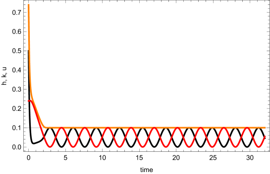
Figure 1: Plot of total energy $h$ (orange), kinetic energy $k$ (black) and potential energy $u$ (red) for an active ergostat and a harmonic multi-particle system. Simulation parameters are: $N=512,d=2,m=1,\omega_{0}=1,\tau_{1}=0.1,\tau_{2}=0.05,T_{init}=0.5,h_{0}=0.1$

See Supplemental Material at [43] for videos of the swarm evolution together with the corresponding histograms of the momenta. The swarm is seen to be oscillating regularly. Each time after a phase of expansion, for a short moment, all particles come to complete rest. Subsequently the swarm continues contracting towards the origin, where it starts expanding again.

6 Active thermostat for a harmonic multi-particle system

In the active thermostat case the time evolution of $\xi$ is given by (28)

$$\dot{\xi}=\frac{1}{\left(\tau_{1}\right)^{2}}\left(\frac{k}{k_{0}}-1\right)-\frac{k}{\tau_{2}\,k_{0}}\xi,\quad k=\frac{1}{N}\sum_{i=1}^{N}\frac{\textbf{p}_{i}^{2}}{2m}$$ (49)

In Fig 2 the kinetic (black), potential (red) and total energies (orange) are plotted, all are oscillating and are exponentially damped.

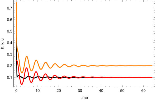
Figure 2: Plot of total energy $h$ (orange), kinetic energy $k$ (black) and potential energy $u$ (red) for an active thermostat and a harmonic multi-particle system. Simulation parameters are: $N=512,d=2,m=1,\omega_{0}=1,\tau_{1}=0.1,\tau_{2}=0.05,T_{init}=0.5,T_{final}=0.1$

The extended system feedback force $\xi$ shows oscillatory behavior and exponential decrease toward $0$, see Fig. 3.

Figure 3: The extended system feedback force $\xi$ for an active thermostat and a harmonic multi-particle system. Simulation parameters are: $N=512,d=2,m=1,\omega_{0}=1,\tau_{1}=0.1,\tau_{2}=0.05,T_{init}=0.5,T_{final}=0.1$

In Fig. 4 the N-particle histogram of the momentum distribution at the initial moment of the simulation is presented. Due to our choice of initial conditions the histogram of the momenta is following closely a pattern related to a Maxwellian distribution (black solid line), corresponding to the initial temperature $T_{init}$.

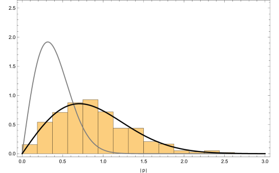
Figure 4: Histogram of the initial momentum distribution for an active thermostat and a harmonic multi-particle system. Simulation parameters are: $N=512,d=2,m=1,\omega_{0}=1,\tau_{1}=0.1,\tau_{2}=0.05,T_{init}=0.5$ (corresponding to the black line), $T_{final}=0.1$ (corresponding to the gray line)

Only a few time steps after the start of the simulation the system reaches the final temperature $T_{final}$, we give a snapshot of the histogram in Fig. 5. The histogram shows a pattern related to a Maxwellian distribution (black solid line), which is corresponding to the final temperature $T_{final}$. See Supplemental Material at [43] for videos of the swarm evolution together with the corresponding histograms of the momenta.

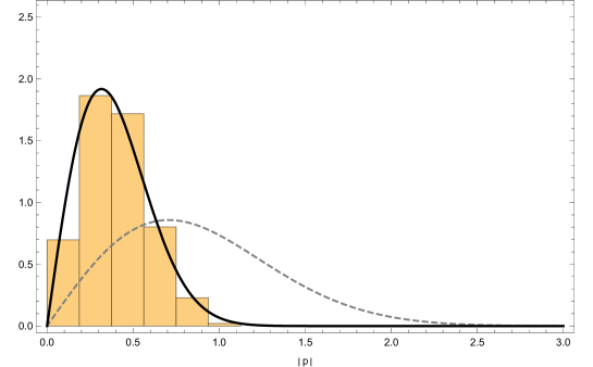
Figure 5: Snapshot of the histogram of the momentum distribution for an active thermostat and a harmonic multi-particle system after thermostatting. Simulation parameters are: $N=512,d=2,m=1,\omega_{0}=1,\tau_{1}=0.1,\tau_{2}=0.05,T_{init}=0.5$ (corresponding to the gray dashed line), $T_{final}=0.1$ (corresponding to the black line)

A precise understanding of the rather complex numerical results in the preceding and the present section can be obtained if we study the harmonic N-particle system in terms of the macroscopic swarm variables (9 - 13). For the active ergostat case we have

$$\dot{k} = {\color[rgb]{0,0,0}-2\sqrt{N}\omega_{0}s-2k\,\xi,}$$ (50)

$$\dot{u} = 2\sqrt{N}\omega_{0}s$$ (51)

$$\dot{s} = \sqrt{N}\omega_{0}k-\sqrt{N}\omega_{0}u-s\,\xi$$ (52)

$$\dot{\xi} = \frac{1}{\left(\tau_{1}\right)^{2}}\left(\frac{h}{h_{0}}-1\right)-\frac{h}{\tau_{2}\,h_{0}}\,\xi,\qquad h=k+u$$ (53)

Linearizing around the stationary point $k\rightarrow k_{0},u\rightarrow u_{0},s\rightarrow s_{0},\xi\rightarrow\xi_{0}$ where

$$k_{0}=u_{0}=\frac{h_{0}}{2},\quad s_{0}=0,\quad\xi_{0}=0$$ (54)

the eigenvalues of the characteristic polynomial read

$$\left\{-\frac{\sqrt{\text{$\tau_{1}$}^{2}-4\text{$\tau_{2}$}^{2}}+\tau_{1}}{2\text{$\tau_{1}$}\text{\text{$\tau_{2}$}}},\frac{\sqrt{\text{$\tau_{1}$}^{2}-4\text{\text{$\tau_{2}$}}^{2}}-\tau_{1}}{2\text{$\tau_{1}$}\text{\text{$\tau_{2}$}}},-2i\sqrt{N}\text{$\omega_{0}$},2i\sqrt{N}\text{$\omega_{0}$}\right\}$$ (55)

The solutions of the linearized system can straightforwardly be obtained, we prefer, however, to give an easy example. We choose

$$\tau_{1}=1,\,\tau_{2}=\frac{1}{2},\,\omega_{0}=\frac{1}{\sqrt{N}}$$ (56)

so that the eigenvalues are simply $\{-1,-1,+i,-i).$ With initial conditions $(k(0),u(0),s(0),\xi(0))=(1,0,0,0)$ and $h_{0}=1$ we find

$$k = \frac{1}{2}+\frac{1}{25}e^{-t}\left(15t+11\right)-\frac{2}{25}\left(\sin(2t)-7\cos(2t)\right)$$ (57)

$$u = \frac{1}{2}+\frac{2}{25}e^{-t}\left(5t+7\right)+\frac{2}{25}\left(\sin(2t)-7\cos(2t)\right)$$ (58)

$$s = -\frac{1}{25}e^{-t}\left(5t+2\right)+\frac{2}{25}\left(7\sin(2t)+\cos(2t)\right)$$ (59)

$$\xi = e^{-t}t$$ (60)

We see that in the active ergostat case $k$ and $u$ have exponentially in the time decreasing contributions but also undamped oscillations. For the total energy $h=k+u$ the undamped oscillatory parts cancel out. Conversely $\xi$ is just exponentially decreasing without oscillations.
 
For the active thermostat case the evolution equations are given by

$$\dot{k} = {\color[rgb]{0,0,0}-2\sqrt{N}\omega_{0}s-2k\,\xi,}$$ (61)

$$\dot{u} = 2\sqrt{N}\omega_{0}s$$ (62)

$$\dot{s} = \sqrt{N}\omega_{0}k-\sqrt{N}\omega_{0}u-s\,\xi$$ (63)

$$\dot{\xi} = \frac{1}{\left(\tau_{1}\right)^{2}}\left(\frac{k}{k_{0}}-1\right)-\frac{k}{\tau_{2}\,k_{0}}\xi$$ (64)

Linearizing around the stationary point $k\rightarrow k_{0},u\rightarrow u_{0},s\rightarrow s_{0},\xi\rightarrow\xi_{0}$ where

$$k_{0}=u_{0}\quad s_{0}=0,\quad\xi_{0}=0$$ (65)

the system again can straightforwardly be solved, yet the solutions are of quite lengthy form. We choose again the special parameter values (56). In this case the eigenvalues become twofold degenerate $\lambda=-1\pm i\sqrt{3}$. Considering once more the initial conditions $(k(0),u(0),s(0),\xi(0))=(1,0,0,0)$ and choosing $k_{0}=1$ the solutions of the linearized dynamics are

$$k = 1+\frac{1}{3}e^{-t}\left(\sqrt{3}(2-3t)\sin\left(\sqrt{3}t\right)-3(t-1)\cos\left(\sqrt{3}t\right)\right)$$ (66)

$$u = 1+\frac{1}{3}e^{-t}\left(\sqrt{3}(t+1)\sin\left(\sqrt{3}t\right)-3t\cos\left(\sqrt{3}t\right)\right)$$ (67)

$$s = \frac{1}{3}e^{-t}t\left(\sqrt{3}\sin\left(\sqrt{3}t\right)+3\cos\left(\sqrt{3}t\right)\right)$$ (68)

$$\xi = -\frac{4e^{-t}(t-1)\sin\left(\sqrt{3}t\right)}{\sqrt{3}}$$ (69)

All quantities show exponentially damped oscillations.

Finally we apply our analysis the Nosé–Hoover thermostat. In this case one has

$$\dot{k} = {\color[rgb]{0,0,0}-2\sqrt{N}\omega_{0}s-2k\,\xi,}$$ (70)

$$\dot{u} = 2\sqrt{N}\omega_{0}s$$ (71)

$$\dot{s} = \sqrt{N}\omega_{0}k-\sqrt{N}\omega_{0}u-s\,\xi$$ (72)

$$\dot{\xi} = \frac{1}{\left(\tau_{1}\right)^{2}}\left(\frac{k}{k_{0}}-1\right)$$ (73)

It is well known that in the Nosé–Hoover case no stable fixed points are existing. This is easily demonstrated by linearizing around the stationary point $k\rightarrow k_{0},u\rightarrow u_{0},s\rightarrow s_{0},\xi\rightarrow\xi_{0}$ where

$$k_{0}=u_{0}\quad s_{0}=0,\quad\xi_{0}=0$$ (74)

One finds the strictly imaginary eigenvalues

$$\left\{\pm i\frac{\sqrt{\sqrt{4N^{2}\text{$\tau_{1}$}^{4}\text{$\omega_{0}$}^{4}+1}+2N\text{$\tau_{1}$}^{2}\text{$\omega_{0}$}^{2}+1}}{\tau_{1}},\pm i\frac{\sqrt{-\sqrt{4N^{2}\text{$\tau_{1}$}^{4}\text{$\omega_{0}$}^{4}+1}+2N\text{$\tau_{1}$}^{2}\text{$\omega_{0}$}^{2}+1}}{\tau_{1}},\right\}$$ (75)

so all macroscopic swarm variables are showing undamped oscillations.

7 Active ergostat for a multi-particle system with Lennard–Jones force

In this section we perform the numerical simulation of an active ergostat for a N-particle system with Lennard–Jones forces. The total Hamiltonian reads

$$H=\sum_{i=1}^{N}\frac{\textbf{p}_{i}^{2}}{2m}+\frac{1}{2}\sum_{i,j=1}^{N}\epsilon\left(\left(\frac{a}{\mid\textbf{x}_{i}-\textbf{x}_{j}\mid}\right)^{12}-2\left(\frac{a}{\mid\textbf{x}_{i}-\textbf{x}_{j}\mid}\right)^{6}\right).$$ (76)

and the system evolves according to

$$\dot{\textbf{x}}_{i}=\frac{\textbf{p}_{i}}{m},$$ (77)

$$\dot{\textbf{p}}_{i}=-\frac{\partial H}{\partial\mathbf{x_{i}}}-\xi\textbf{p}_{i},$$ (78)

$$\dot{\xi}=\frac{1}{\left(\tau_{1}\right)^{2}}\left(\frac{h}{h_{0}}-1\right)-\frac{h}{\tau_{2}\,h_{0}}\,\xi,\quad h=\frac{H}{N}.$$ (79)

The initial conditions are prepared in such a way that CMS coordinates and momenta are vanishing. For the simulation of a Lennard–Jones system it is preferable to choose the initial coordinates randomly from a regular grid within a circle of fixed radius. The initial momenta are taken randomly from a Maxwellian distribution, corresponding to some chosen initial temperature $T_{init}$.

First we study ergostatting for a small particle number N=8. In Fig. 6 a plot of the kinetic (black), potential (red) and total (orange) energy is given.

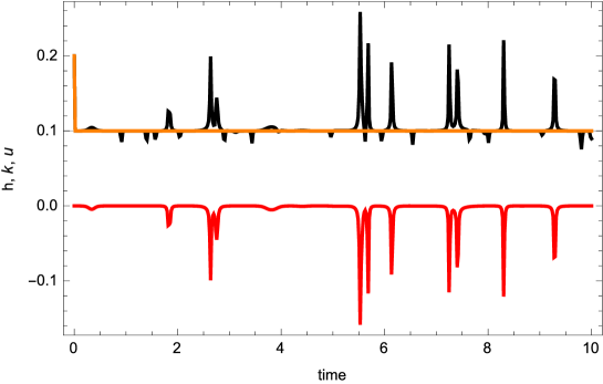
Figure 6: Plot of total energy $h$ (orange), kinetic energy $k$ (black) and potential energy $u$ (red) for an active ergostat and a Lennard–Jones multi-particle system. Simulation parameters are: $N=8,d=2,m=1,a=0.05,\varepsilon=1,\tau_{1}=0.1,\tau_{2}=0.05,T_{init}=0.2,h_{0}=0.1$

We find that the total energy $h$ is quickly fixed at its required value $h_{0}$. The clearly pronounced positive spikes in the kinetic energy and the coinciding negative spikes in the potential energy correspond to events where two particles find themselves sufficiently close one to another. The potential energy of the system receives a negative contribution which due to the ergostatting mechanism leads to an increase of the kinetic energy, which prevents clusterization. The small negative spikes in the kinetic energy are a consequence of the interaction of the particles with the external potential that is introduced to prevent the swarm from spreading apart. For simplicity we did not include the plot of the external potential.

The extended system feedback force $\xi$ is vanishing in good approximation after a very short moment and the system approximately becomes Hamiltonian. As now the conservation of the total energy is guaranteed by the Hamiltonian dynamics itself, ergostatting due to the extended system feedback force $\xi$ has only minor importance.

When studying a system with $N=128$ particles the above features and interpretations get somewhat washed out. It can clearly be seen again that the system quickly achieves the required total energy $h_{0}.$ The kinetic energy $k$ and the averaged potential energy $u$ of the system are fluctuating quite heavily, yet their sum $h=k+u$ is stabilized well, see Fig. 7.

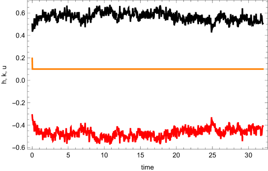
Figure 7: Plot of total energy $h$ (orange), kinetic energy $k$ (black) and potential energy $u$ (red) for an active ergostat and a Lennard–Jones multi-particle system. Simulation parameters are: $N=128,d=2,m=1,a=0.05,\varepsilon=1,\tau_{1}=0.1,\tau_{2}=0.05,T_{init}=0.5,h_{0}=0.1$

The extended system feedback force is fluctuating at a small order of magnitude, see Fig. 8.

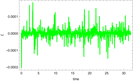
Figure 8: Plot of extended system feedback force $\xi$ for an active ergostat and a Lennard–Jones multi-particle system. Simulation parameters are: $N=128,d=2,m=1,a=0.05,\varepsilon=1,\tau_{1}=0.1,\tau_{2}=0.05,T_{init}=0.5,h_{0}=0.1$

See Supplemental Material at [43] for videos of the swarm evolution together with the corresponding histograms of the momenta.

8 Active thermostat for a multi-particle system with Lennard–Jones force

We perform the simulation of an active thermostat for a N-particle system with the Lennard–Jones Hamiltonian (76) and the time evolution (77), (78) and (28).

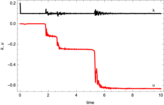
Figure 9: Plot of kinetic energy $k$ (black) and potential energy $u$ (red) for an active thermostat and a Lennard–Jones multi-particle system. Simulation parameters are: $N=8,d=2,m=1,a=0.05,\varepsilon=1,\tau_{1}=0.1,\tau_{2}=0.05,T_{init}=0.2,T_{final}=0.1$

Again we first study the case of small particle numbers, choosing N=8. We observe that $k$ quickly reaches the prescribed stationary value $k_{0}$, while $u$ shows synchronized stepwise transitions towards lower values. In Fig. 9 the kinetic (black) and potential (red) energies are plotted. Each transition corresponds to the formation of a cluster of a pair of particles or of additional particles joining an already existing cluster. As each binding of a particle adds an amount of negative potential energy to the system, the total energy h decreases accordingly. If all particles would form one big cluster, the kinetic energy of the whole system would divide itself between the centre of mass motion / rotation of the cluster and the vibrations of all the bound particles.

The extended system feedback force $\xi$ is stabilizing the kinetic energy $k$ by bursts of fluctuations, this can be seen in Fig. 10.

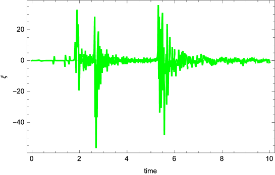
Figure 10: Plot of extended system feedback force $\xi$ for an active thermostat and a Lennard–Jones multi-particle system. Simulation parameters are: $N=8,d=2,m=1,a=0.05,\varepsilon=1,\tau_{1}=0.1,\tau_{2}=0.05,T_{init}=0.2,T_{final}=0.1$

In a simulation of the Lennard-Jones gas with particle number N=512 the main features of our analysis persist, see Fig. 11 for plots of the kinetic (black) and potential (red) energies.

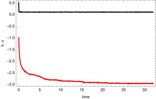
Figure 11: Plot of kinetic energy $k$ (black) and potential energy $u$ (red) for an active thermostat and a Lennard–Jones multi-particle system. Simulation parameters are: $N=512,d=2,m=1,a=0.05,\varepsilon=1,\tau_{1}=0.1,\tau_{2}=0.05,T_{init}=0.5,T_{final}=0.1$

The extended system feedback force $\xi$ is fluctuating qualitatively similar as in Fig. 8, maintaing a constant value of the kinetic energy. Also when plotting the N-particle histograms of the momentum distribution similar figures as previously are obtained, see Fig. 4 and Fig. 5.

Finally we demonstrate that for sufficiently low temperatures the thermostatted Lennard–Jones gas is forming clusters. The snapshots were taken at the initial time and at three consecutive moments, see Fig. 12.

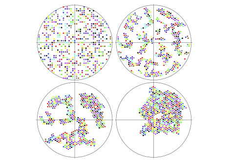
Figure 12: Cluster formation in a thermostatted Lennard–Jones gas. Simulation parameters are: $N=512,d=2,m=1,a=0.05,\varepsilon=1,\tau_{1}=0.1,\tau_{2}=0.05,T_{init}=0.5,T_{final}=0.1$

See Supplemental Material at [43] for videos of the cluster formation together with the corresponding histograms of the momenta.

9 Outlook

A novel type of ergostatting and thermostatting at fixed points of the evolution of particle swarms has been presented in this paper and shown to be viable and useful. We are convinced that various generalizations and a new arena of exciting applications will open up.

First we plan to check the efficiency of our thermostat / ergostat for Lennard - Jones gas simulations by carefully comparing its performance with other more conventional thermostats. In dependence of the relaxation times $\tau_{1},\tau_{2}$ we will study - among others - variances of the total energy, total kinetic energy and the extended system feedback force $\xi$ [44].

It seems immediately possible to formulate stochastic variants [20, 21, 22] of our fixed point method and compare simulations with other stochastic schemes [45].

A further possibility would be to extend our method to isobaric or isothermal–isobaric ensembles [2, 46, 47, 48], where the system not only exchanges heat with the thermostat, but also volume and work with the barostat. For a Lennard–Jones gas one could study phase transitions and the formation of clusters.

In a different approach we envisage to adapt our scheme to the Nosé– Hoover chain construction [13], which could be interesting especially for thermostatting small or stiff systems.

As a final suggestion it appears interesting to examine our fixed point method specifically in nonequilibrium conditions, where it might be advantageous to control total energy relative to just total kinetic energy.

References

- [1] L. V. Woodcock, Isothermal molecular dynamics calculations for liquid salts, Chem. Phys. Lett. 10, 257 ( 1971)
- [2] H. C. Andersen, Molecular dynamics simulations at constant pressure and/or temperature, J. Chem. Phys. 72, 2384 (1980).
- [3] S. Nosé, A Molecular Dynamics Method for Simulations in the Canonical Ensemble, Molecular Physics 52, 255-268 (1984).
- [4] S. Nosé: A unified formulation of the constant temperature molecular-dynamics methods, J. Chem. Phys. 81, 511 (1984).
- [5] S. Nosé, Constant Temperature Molecular Dynamics Methods, Progress in Theoretical Physics Supplement 103, 1-46 (1991).
- [6] W. G. Hoover, Canonical dynamics: Equilibrium phase-space distributions, Phys. Rev. A 31, 1695 (1985).
- [7] H. A. Posch, W. G. Hoover, and F. J. Vesely, Canonical dynamics of the Nosé oscillator: Stability, order, and chaos, Phys. Rev. A 33, 4253 (1986).
- [8] D. Kusnezov, A. Bulgac, and W. Bauer, Canonical Ensembles from Chaos, Ann. Phys. 204, 155-185 (1990).
- [9] D. Kusnezov, and A. Bulgac, Canonical Ensembles from Chaos: Constrained Dynamical Systems, Ann. Phys. 214, 180-218 (1992).
- [10] J. Jellinek, and R. S. Berry, Generalization of Nosé’s Isothermal Molecular Dynamics, Phys. Rev. A 38, 3069-3072 (1988).
- [11] A. C. Branka, and K. W. Wojciechowski, Generalization of Nosé and Nosé-Hoover Isothermal Dynamics, Phys. Rev. E 62, 3281-3292 (2000).
- [12] A. C. Branka, M. Kowalik, and K. W. Wojciechowski, Generalization of the Nosé–Hoover approach, J. Chem. Phys. 119, 1929 (2003).
- [13] G. J. Martyna, M. L. Klein, and M. E. Tuckerman, Nosé–Hoover chains: The canonical ensemble via continuous dynamics, J. Chem. Phys. 97, 2635 (1992)
- [14] H. J. C. Berendsen, J. P. M. Postma, W. F. van Gunsteren, A. DiNola, and J.R. Haak, Molecular-Dynamics with Coupling to an External Bath, J. Chem. Phys. 81, 3684 (1984).
- [15] W. G. Hoover , A. J. C. Ladd, and B. Moran, High-strain-rate plastic flow studied via nonequilibrium molecular dynamics Phys. Rev. Lett. 48, 1818 (1982).
- [16] D. J. Evans, Computer ‘experiment’ for nonlinear thermodynamics of Couette flow, J. Chem. Phys. 78, 3297 (1983) .
- [17] C. P. Dettmann, and G. P. Morriss, Hamiltonian Formulation of the Gaussian Isokinetic Thermostat, Phys. Rev. E 54, 2495-2500 (1996).
- [18] C. P. Dettmann, Hamiltonian for a restricted isoenergetic thermostat, Phys. Rev. E 60, 7576 (1999).
- [19] S. Bond, B. Laird, and B. Leimkuhler, The Nosé-Poincaré Method for Constant Temperature Molecular Dynamics, Journal of Computational Physics 151, 114-134 (1999).
- [20] B. Leimkuhler, E. Noorizadeh, and F. Theil, A gentle stochastic thermostat for molecular dynamics, J. Stat. Phys. 135, 261 (2009).
- [21] A. A. Samoletov, C. P. Dettmann, and M. A. J. Chaplain, Thermostats for “slow” configurational modes, J. Stat. Phys. 128, 1321 (2007).
- [22] B. Leimkuhler, Generalized Bulgac–Kusnezov methods for sampling of the Gibbs– Boltzmann measure, Phys. Rev. E 81, 026703 (2010).
- [23] G. Bussi, D. Donadio, and M. Parrinello, Canonical sampling through velocity rescaling, J. Chem. Phys. 126, 014101 (2007).
- [24] G. Bussi and M. Parrinello, Accurate sampling using Langevin dynamics, Phys. Rev. E 75, 056707 (2007).
- [25] G. Bussi, and M. Parrinello, Stochastic thermostats: comparison of local and global schemes, Computer Physics Communications 179, 26 (2008).
- [26] M. Ceriotti, M. Parrinello, T. E. Markland, and D. E. Manolopoulos, Efficient stochastic thermostatting of path integral molecular dynamics, J. Chem. Phys. 133, 124104 (2010).
- [27] R.Klages, Microscopic Chaos, Fractals and Transport in Nonequilibrium Statistical Mechanics, monograph, Advanced Series in Nonlinear Dynamics Vol.24 (World Scientific, Singapore, 2007).
- [28] B. Leimkuhler, and C. Matthews, Molecular Dynamics With Deterministic and Stochastic Numerical Methods (Springer, Berlin 2015).
- [29] W. G. Hoover, and C. G. Hoover, Simulation and Control of Chaotic Nonequilibrium Systems, Advanced Series in Nonlinear Dynamics Vol.27 ( World Scientific, Singapore, 2015).
- [30] J. Toner, Y. Tu, and S. Ramaswami, Ann. Phys. 318, 170 (2005).
- [31] P. Romanczuk, M. Bär, W. Ebeling, B. Lindner, and L. Schimansky-Geier, Active Brownian particles: From individual to collective stochastic dynamics, Eur. Phys. J. Special Top. 202, 1 (2012).
- [32] T. Vicsek, and A. Zafeiris, Collective motion, Phys. Rep. 517, 71 (2012).
- [33] L. Schimansky-Geier, M. Mieth, H. Rose, and H. Malchow, Structure formation by active Brownian particles, Phys. Lett. A 207, 140 (1995).
- [34] F. Schweitzer, W. Ebeling, and B. Tilch, Complex Motion of Brownian Particles with Energy Depots, Phys. Rev. Lett. 80, 5044 (1998).
- [35] F. Schweitzer, Brownian Agents and Active Particles (Springer, Berlin, 2003).
- [36] W. Ebeling, I. M. Sokolov, Statistical Thermodynamics and Stochastic Theory of Nonequilibrium Systems (World Scientific, Singapore, 2005).
- [37] A. Glück, H. Hüffel, and S. Ilijić, Swarms with canonical active Brownian motion, Phys. Rev. E 83, 051105 (2011).
- [38] A. Glück, H. Hüffel, and S. Ilijić, Canonical active Brownian motion, Phys. Rev. E 79, 021120 (2009).
- [39] F. Schweitzer, W. Ebeling, and B. Tilch, Statistical mechanics of canonical-dissipative systems and applications to swarm dynamics, Phys. Rev. E 64, 021110 (2001).
- [40] A. Khinchin, Mathematical Foundations of Statistical Mechanics (Dover Publications, New York, 1949).
- [41] P Castiglione, M Falcioni, A Lesne, and A Vulpiani, Chaos and Coarse Graining in Statistical Mechanics (Cambridge University Press, Cambridge, 2008).
- [42] W. G. Hoover, J. C. Sprott, and C. G. Hoover, Ergodicity of a singly-thermostated harmonic oscillator, Commun Nonlinear Sci Numer Simulat 32, 234 (2016) .
- [43] http://sail.zpf.fer.hr/active/thermostat
- [44] H. Hüffel, S. Ilijić, and M. Neumann, in preparation.
- [45] B. Leimkuhler, E. Noorizadeh, and O. Penrose, Comparing the Efficiencies of Stochastic Isothermal Molecular Dynamics Methods, J. Stat. Phys. 143, 921 (2011).
- [46] W. G. Hoover, Constant-pressure equations of motion, Phys. Rev. A 34, 2499 (1986).
- [47] G. J. Martyna, D. J. Tobias, and M. L. Klein, Constant pressure molecular dynamics algorithms, J. Chem. Phys. 101, 4177 (1994).
- [48] M.E. Tuckerman, Y. Liu, G. Ciccotti, and G. J. Martyna, Non-Hamiltonian molecular dynamics: Generalizing Hamiltonian phase space principles to non-Hamiltonian systems, J. Chem. Phys. 115, 1678 (2001).