Full-scale Cascade Dynamics Prediction with a Local-First Approach

Abstract

Information cascades are ubiquitous in various social networking web sites. What mechanisms drive information diffuse in the networks? How does the structure and size of the cascades evolve in time? When and which users will adopt a certain message? Approaching these questions can considerably deepen our understanding about information cascades and facilitate various vital applications, including viral marketing, rumor prevention and even link prediction. Most previous works focus only on the final cascade size prediction. Meanwhile, they are always cascade graph dependent methods, which make them towards large cascades prediction and lead to the criticism that cascades may only be predictable after they have already grown large. In this paper, we study a fundamental problem: full-scale cascade dynamics prediction. That is, how to predict when and which users are activated at any time point of a cascading process. Here we propose a unified framework, FScaleCP, to solve the problem. Given history cascades, we first model the local spreading behaviors as a classification problem. Through data-driven learning, we recognize the common patterns by measuring the driving mechanisms of cascade dynamics. After that we present an intuitive asynchronous propagation method for full-scale cascade dynamics prediction by effectively aggregating the local spreading behaviors. Extensive experiments on social network data set suggest that the proposed method performs noticeably better than other state-of-the-art baselines.

1 Introduction

Online social networks provide platforms for people in where they can easily share and discuss ideas and innovations. In this setting, people react to information on the basis of their neighbors’ behavior, and the people in contact with them act in a same way. Thus information cascades naturally form and become common in online social networks. In consideration of the impact of information cascades on online social networks, uncovering how information cascades in the networks can considerably deepen our understanding about information cascades and facilitate various vital applications, including viral marketing, spreading suppression and even link prediction. A growing body of researches has focused on the statistical properties of information cascades or the common patterns in temporal dynamics [1-5]. As a nontrivial line of work, information cascades prediction has aroused considerable research interests recently. Traditional models (independent cascade or threshold model) are usually designed for all diffusion processes, regardless of the nature of the diffusion objects. However, recent studies [1, 2] show that the assumption that most of the models followed becomes unreasonable for information cascades in online social networks, and the information cascades, as the fundamental collective dynamics of social networks, have strong relevance to complex contagion mechanisms.

Availability of large scale data about information cascades has facilitated the study of predictive models, and many approaches have been developed recently, including model-centric methods [6-8] and empirical methods [9-14]. Most of the previous methods try to distinguish between messages with different popularity and assume that the cascade graph (i.e. the path and user information of information cascades.) in early stage is available. They are biased towards studying extremely large but also extremely rare cascades, by passing the whole issue about the general predictability of cascades. However, because very limited cascade information can be obtained for newly created cascades and storing complete cascade graph may not be feasible as the size of cascades grows, the cascade graph based methods may be impracticable in real-life applications. Moreover, the real-life applications always care about not solely the final cascade size, but also the whole issue of information cascades. These challenges reinforce the fact that finding an effective way to predict when and which users will be activated at any time point of the entire lifetime of cascades regardless of the cascade graph size remains a big task to date.

The proposed full-scale cascade dynamics prediction is different from the traditional cascades prediction problems. Except for the difference between the core aims of the proposed problem and the traditional cascades prediction, as discussed above, the overriding concern of the proposed problem is to evaluate all possible factors and measure principal driving mechanisms by capturing the effective information and the intrinsic relations between them, while the focus of the classical problem is the design of discriminative features. Moreover, the proposed problem calls for a common computational framework that is independent of data features, which is much more general than the traditional problems designed for certain types of information in various real-life networks.

The full-scale cascade dynamics prediction presents several challenges. First, hybridity, information cascades are driven by the social interactions between users with various confounding factors, which makes it difficult to be modeled comprehensively and effectively. That is, various factors are considered in previous methods [9, 10, 11, 14], and how to comprehensively study and identify the effective factors is a big challenge. Second, incomplete, in this paper, we argue that getting global scenes of information flows is usually unfeasible, which makes the problem nontrivial. Therefore, how to effectively capture the whole issue of information cascades with little global cascade information becomes a significant challenge. Third, generality, it is important to develop a model that can adapt well to different types of social media, including blogging, e-mail, social sites, etc.

In light of these differences and challenges, we define “spreading behaviors” to represent the personal interactions and behaviors at microscopic level and assume that the macroscopic information cascades are generated from the spreading behaviors at microscopic level. Thus, the task of full-scale cascade dynamics prediction can be decomposed into a set of spreading behavior estimation tasks with network topology, and the availability of cascade graphs in early stage is no longer the prerequisite for information cascades prediction. Based on the above analysis, this paper proposes a unified two-phase framework FScaleCP to predict full-scale cascade dynamics. At the first phase, it leverages supervised learning to model local spreading behaviors by capturing the joint action of factors from multiple dimensions and quantitatively selects the most effective feature space and spreading behavior estimation model. At the second phase, Inspired by the work on label propagation algorithm [15], we incorporate the spreading behavior estimation model into local network topology and propose a flexible and robust supervised asynchronous propagation method to aggregate the local spreading behaviors for full-scale cascade dynamics prediction. Figure 1 gives an illustration of information cascade dynamics prediction. The main contributions of this work include: (1) we formally define a novel problem of full-scale cascade dynamics prediction in networks and propose a unified FScaleCP framework to solve it; (2) we propose a supervised asynchronous propagation method to incorporate the local spreading behaviors for predicting cascade dynamics in social network. To estimate the local spreading behaviors, we adopt the supervised learning model and feature selection method to utilize implicit and confounding factors; (3) experimental results on social network data set demonstrate that the proposed FScaleCP significantly outperforms several state-of-the-art information cascades prediction algorithms. Together, these contributions would promote the understanding of how information cascades across network and suggest new directions for modeling and optimization of information cascades.

The remainder of this paper is organized as follows. Section 2 presents related works about information cascades. Section 3 formalizes the full-scale cascade dynamics prediction problem in social networks. Section 4 details the proposed framework. Section 5 explains the experimental results. Section 6 concludes the work.

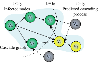
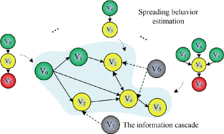
Figure 1: Illustrate of information cascade dynamics prediction. (a) Cascading Process; (b) Behavioral dynamics estimation based cascade dynamics prediction, in which nodes denote network users and dashed lines represent inter-relationships. In the network, the evolution of information flows (solid lines) is predicted based on atomic spreading behavior estimation tasks. Meanwhile, all nodes update their network behaviors asynchronously on the basis of the actions of their surroundings.

2 Related work

In this section we review some important researches that are close related to our work, regarding social influence computation, individual spreading behavior estimation, as well as information cascades prediction problem.

Social influence. Social influence accompanies transferring information from one user to the other. It is a key to explain information cascades in social networks. A crucial task in the analysis of social influence is to find evidence of influence and distinguish influence from homophily or unobserved confounding variables. Shuffle test [16] is proposed to detect a signal of influence based on the intuition that if influence is not a likely source of correlation in a system, timing of actions should not matter, and therefore reshuffling the time stamps of the actions should not significantly change the amount of correlation. Investigations on the interplay between social influence and homophily using data from Wikipedia have been made by Crandallet et al. [17]. S. Aral et al. [18] develop a dynamic matched sample estimation framework to distinguish influence and homophily effects in dynamic networks. Moreover, all viral marketing papers assume they have a social graph with edges labeled with probabilities of influence between users as input. To our knowledge, the question of how or from where one can compute the influence probabilities has been largely left open. Amit Goyal et al. [19] study how to learn cascade probabilities from a log of past propagations, and they propose both static and time-dependent models for capturing influence. Tang et al. [20] propose a topic factor graph model to measure the strength of topic-level social influence quantitatively.

Individual spreading estimation. A bulk of studies attempt to understand individual spreading behaviors in terms of decay effects [21], memory effect [22], social reinforcement [22, 23], etc. Moreover, some other works show that limited attention [24, 25] and semantic similarity [24] are also important indicators. With limited attention, information is less likely to be noticed by users as the volume of information scales with the number of user’s parents. Meanwhile, users tend to spread the information with similar semantic meaning to their history information. Besides, Tang et al. [26] study the effects of pairwise influence and structure influence on user’s spreading behaviors. As the focus of the existing works is to explore whether a factor is effective in spreading behavior estimation, rather than modeling spreading behavior as accurate as possible, the prediction accuracy they produce is less reliable and there is no knowledge about the importance of every factor.

Information cascades prediction. Information cascades prediction has broad application range, including item recommendation, viral marketing, spreading suppression, etc. It is the research area that is most relevant to our work. Many theoretical model based methods are developed to capture the cascading process [6-8]. As the complexity limitation and many assumptions being included, the methods may hard to consider the complex contagion mechanisms comprehensively, and their solutions are generally not applicable in real-life situations. On the other hand, to predict the future popularity of a meme, Weng et al. [9] develop a model considering early cascade patterns based community concentration, influence of early adopters and time series characteristics. Ma et al. [10] propose a supervised learning based method to predict the range of the popularity of new hashtags in Twitter. It extracts content features from hashtag string and the collection of tweets and contextual features from cascade graph. Hong et al. [11] formulate the task of predicting the popularity of messages into a multi-class classification problem by investigating content features, temporal features, as well as structural properties of cascade graph. Kupavskii et al. [12] try to forecast how many retweets a given tweet will gain during a fixed time period since the initial moment. Tsur et al. [13] also study the diffusion of information in Twitter and predict the hashtag popularity by combining content features with temporal and topological features. Cheng et al. [14] focus on a some different problem. Rather than to predict the final cascade size, they instead to predict whether the cascade size of the next stage will bigger than the median site and seek to understand how predictability varies along the entire lifetime of cascade. They are aware of the dependency of early cascade graphs and the bias of extremely large cascades, but they don’t solve the problem thoroughly.

Summary. To the best of our knowledge, our work is the front-runner to propose that modeling full-scale cascade dynamics indirectly using local spreading behavior estimation, which optimize the generality of cascade prediction method and capture the whole issue of information cascades. This distinguishes our work from the existing studies that merely consider the final size prediction of extremely large but also extremely rare cascades.

3 Problem formulation

Generally, we use $G=(V;E)$ to denote a social network, where $V=\{v_{i}\}$ is the set of nodes which represent social users, and $E\subseteq V\times V$ is the set of directed edges which are mapped to links between social users. $e_{ij}=(v_{i},v_{j})\in E$ means there is a direct link from node $v_{i}$ to $v_{j}$ in $G$ and $e_{ij}\notin E$ represents that there is no such a direct link. To a directed edge $e_{ij}$, we define node $v_{j}$ is the parent of node $v_{i}$ and node $v_{i}$ is the child of node $v_{j}$, and $v_{i}$ is exposed to the messages published by $v_{j}$. Then we define $P_{i}$ to represent the parent node set of node $v_{i}$ and $C_{i}$ to represent the child node set of node $v_{i}$. Moreover, if node $v_{j}$ is a parent of node $v_{i}$ and node $v_{i}$ is also a parent of node $v_{j}$, we say they are friends.

Definition 1 (Activated nodes).

Given node $v_{j}$ and its child node $v_{i}$, if node $v_{j}$’s action associated to a message induce her child $v_{i}$ to act in a similar way, we say that the child node $v_{i}$ becomes “activated” to the message, otherwise “inactivated”. For each activated node $v_{i}$, we assume all its activated parent nodes before $v_{i}$ influenced her, and we define all these activated parent nodes in $P_{i}$ as activated parent set $AP_{i}$ of node $v_{i}$.

Definition 2 (Information cascade).

Given network $G$ and a node being activated to a message $m$ at $t_{0}$. The message cascades through the network with exposed child nodes become activated at $t_{1}>t_{0}$, thereby exposing their own child nodes to the message, and so on. By repeating the process, an information cascade is typically formed.

Definition 3 (Activation sequence).

Given network $G$ and an information cascade corresponding to a message $m$, a set of nodes $\{v_{i}\}$ capturing the order in which the network nodes adopted the message $m$ is called the activation sequence of the cascade.

According to the above definitions, a information cascade can be represented by an activation sequence as $C_{m}=\{v_{1},v_{2},...,v_{k}\}$. The time stamp that node $v_{i}$ gets activated to the information is $t(v_{i})$, $t(v_{i})\leq t(v_{i+1})$. We denote the time stamp sets corresponding to the activated parent set $AP_{i}$ and the activation sequence $C_{m}$ as $APt_{i}$ and $Ct_{m}$ respectively. Then the partially observed cascade before time $t$ can be denoted as $C_{m}(t)=\{v_{i}|t(v_{i})<t\}$, and the cascade size can be defined as $|C_{m}(t)|$, where $|\cdot|$ is the cardinality of a set. Moreover, we assume that the node which was already activated to a message cannot be re-activated or inactivated to the message.

Definition 4 (History message set).

If node $v_{i}$ was activated to a message $m$, we say that message $m$ is one of the history messages of node $v_{i}$. We explore history message set $HM_{i}$ to represent all the history messages of node $v_{i}$.

Definition 5 (Candidate message set).

If activated parent set $AP_{i}$ is not empty, node $v_{i}$ is exposed to the messages published by the activated parent nodes in $AP_{i}$. As $v_{i}$ is possible to be activated to the messages, we define the messages as candidate message set $CM_{i}$ of $v_{i}$.

Problem 1 (Full-scale cascade dynamics prediction in social networks).

Given a network $G$, any time point $t$, partially observed information cascade $C_{m}(t)$ before time $t$, the goal is to propose a predictive framework based on $G$ and $C_{m}(t)$ such that the framework can predict the activated node set $ANSet_{t^{\prime}}$ and the cascade size $|ANSet_{t^{\prime}}|$ at any later time $t^{\prime}>t$ in the entire life of the cascade.

4 Full-Scale Cascade Dynamics Prediction Framework

In this section, we first introduce the framework to solve the proposed full-scale cascade dynamics prediction problem in social networks, and then explain the two main phases in the framework respectively. Finally, we present FScaleCP properties and complexity analysis.

4.1 FScaleCP Framework

To solve the challenges of full-scale cascade dynamics prediction, we propose a framework, FScaleCP (shown in Figure 2), to first model the local spreading behaviors, from which we then design a global function for aggregating the local behavioral dynamics to approximate the cascade dynamics in social network. Except for the vivid way to cascades prediction, FScaleCP provides an intuitive and comprehensive image to model the real-world network dynamics.

At the first phase, given network $G$ and history cascade set $\{C_{1},C_{2},...,C_{n}\}$, we propose a predictive model to estimate the local spreading behaviors of inactivated nodes based on the optimal feature space and model parameters. The motivation is that when users spread messages, the exhibited behavioral patterns lead to information redundancy that can be captured in terms of data features. Following the machine learning research, we can learn an estimation model by exploring a supervised learning framework that utilizes the features.

At the second phase, based on the proposed spreading behavior estimation model and partially observed cascade $C_{m}(t)$, we propose an algorithm to predict the cascade conditions of message $m$ at time $t^{\prime}$. The idea is that the practical information cascading process can be reproduced approximately by iterative propagation on local network topology.

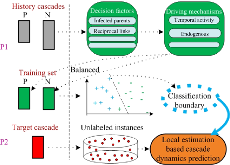
Figure 2: Full-Scale Cascade Dynamics Prediction Framework (FScaleCP).

4.2 Local Behavioral Dynamics Estimation Model

In this section, we assume a social media site’s users have common and consistent behavioral patterns, and they combine their personal attributes and surrounding conditions to handle the candidate messages. The information redundancies resulted by common and consistent behavioral patterns can be utilized to identify their behavior patterns in information diffusion process. Of course, individuals can avoid such information redundancies by random their response behaviors deliberately, such as selecting a completely different responding behavior to similar messages and surrounding conditions. Unfortunately, all of these requirements are contrary to practical needs and human abilities. So this property can be explored to help learn a spreading behavior estimation model.

4.2.1 Local Conditions Analysis and Driving Mechanism Definition

In this study, we will analyze multiple driving mechanisms of information diffusion to harness the redundant information, which include (a) Content semantic driving mechanism (2) Temporal activity driving mechanism (3) Network structural driving mechanism (4) Endogenous driving mechanism.

Content semantic driving mechanism. Common sense dictates that the candidate messages $CM_{i}$ and the history messages $HM_{i}$ all may influence users’ responses in social networks. That is, the content and the semanteme of the messages may drive users to spread messages or not. In the candidate messages, keywords can help users to identify core topics quickly, which can make messages avoid being flooded by the continual stream of new messages. Moreover, more longer the candidate messages, more information is contained in them, and more possible to arouse users’ interests to spread them. In addition, users’ history messages can hint for their personal interest. More broad interest diversity of a user, more likely he become interested in a random message and spread it. Finally, more closely a candidate message’s topic matches user’s interest, more possible the user spread it. Combining the above factors, we define the content semantic mechanism $\mathcal{CSM}(t)$ at time $t$ as follows:

$${\mathcal{CSM}(t)}=f_{csm}(KeyW_{m},ContLen_{m},IntDiv_{u},IntSim_{m})$$ (1)

where $ContLen_{m}$ is the length of a message, $KeyW_{m}$ is a boolean value to denote the existence of keywords in message. $IntDiv_{u}$ is the diversity of user interest computed by Shannon entropy $IntDiv_{u}=-\sum\nolimits_{i}{I_{u}(i)\log I_{u}(i)}$, where $I_{u}(i)$ is the probability value of topic $i$ in user $u$’s interest. $IntSim_{m}$ is the semantic similarity between user interest and the candidate message computed by Jensen-Shannon divergence $IntSim(I_{u},T_{m})=\frac{{D(I_{u}||T_{m})+D(T_{m}||I_{u})}}{2}$, where $D(T_{m}||I_{u})=\sum\nolimits_{i}{T_{m}(i)*In(T_{m}(i))/I_{u}(i)}$ is the Kullback-Leibler divergence between distribution $T_{m}$ and $I_{u}$, $T_{m}$ is the topic distribution of the candidate message computed by LDA [27], $I_{u}$ is the average topic distribution of all history messages of user $u$.

Temporal activity driving mechanism. The rationale for taking a close look at this dimension is that messages are time-sensitive, and their novelty and influence would decline with the increase of time delay. Intuitively, for any appealing message, most of users would likely to forward it as soon as possible to improve their social influence. In other words, people may lose interests to forward the messages that have been around for a long time. Considering activation sequence $C_{m}$ and its time stamps $Ct_{m}$, we define the temporal activity driving mechanism $\mathcal{TAM}(t)$ at time $t$ as follows:

$${\mathcal{TAM}(t)}=f_{tam}(AvgExpT_{m},SurT_{m},AvgFordD_{m})$$ (2)

where $AvgExpT_{m}$ is the average exposure time of candidate message $m$ on $AP_{i}$, $SurT_{m}$ is the survival time characterizing the novelty of message $m$, and $AvgFordD_{m}$ is the average forward delay between every two successively activated nodes for message $m$’s appealing degree measure.

Surrounding conditions driving mechanism. We notice that the actions of friends would influence the user behaviors. According to reality experience, close friends are always have much more influence on users than ordinary friends. Moreover, the study in [28] shows that repeated exposures have impact on information spreading. Thus we study the influence of parents number, relationship type and the ratio of activated parents on user behaviors, and we define the surrounding conditions driving mechanism $\mathcal{SCM}(t)$ as follows:

$${\mathcal{SCM}(t)}=f_{scm}(SocialRe_{u},SocialReR_{u},ActRecRel_{u},ActRecRelR_{u},RecRel_{u},RecRelR_{u})$$ (3)

where $SocialRe_{u}$, $ActRecRel_{u}$ and $RecRelR_{u}$ are the number of activated parents, reciprocal activated parents and reciprocal parents respectively, $SocialReR_{u}$ is the ratio of $SocialRe_{u}$ to the number of parents, $ActRecRelR_{u}$ is the ratio of $ActRecRel_{u}$ to $SocialRe_{u}$, and $RecRelR_{u}$ is the ratio of $RecRelR_{u}$ to the number of parents.

Endogenous driving mechanism. Recent research [25] suggests the existing of limitation in human memory and cognition capability. The results demonstrate that human’s attention is limited. Thus, the more number of the candidate messages, the less possibility of a certain message being concerned. Moreover, users’ attributes can be viewed as the hints of user activeness. So we define the endogenous driving mechanism $\mathcal{EM}(t)$ as follows:

$${\mathcal{EM}(t)}=f_{em}(VerSta_{u},ReMsg_{u},ChlNode_{u},AccCreT_{u},CPNodesR_{u})$$ (4)

where $VerSta_{u}$ is verification status of the account of user $u$, $ReMsg_{u}$ is the number of related messages, $ChlNode_{u}$ is the number of child nodes, $AccCreT_{u}$ is the time when the account being created, and $CPNodesR_{u}$ is the ratio of the the number of child nodes to the number of parent nodes.

4.2.2 Local Behavioral Dynamics Estimation

Given network $G$ and current partially observed cascade $C_{m}(t)$, we represent the Local Behavioral Dynamics Estimation Model as $\mathcal{M}_{LBE}(G,C_{m}(t))$. Thus the model can be defined as a function $f(\mathcal{CSM}(t))$, according to the content semantic driving mechanism, $f(\mathcal{TAM}(t))$, according to the temporal activity driving mechanism, and so on. We combine the four driving mechanisms together to represent the final estimation model as $\mathcal{M}_{LBE}(G,C_{m}(t))=f(\mathcal{CSM}(t),\mathcal{TAM}(t)),\mathcal{SCM}(t),\mathcal{EM}(t))$.

There are several ways to substantialize the function $f()$. In this work, from a given network $G$ and a history cascade set $\{C_{1},C_{2},...,C_{n}\}$, each node may was activated to multiple messages. We define each node related with different messages as multiple different spreading instances. Thus we can get two disjoint sets of instances: activated instances $P$ and inactivated instances $I$. Based on the driving mechanisms $\{\mathcal{CSM}(t),\mathcal{TAM}(t)),\mathcal{SCM}(t),\mathcal{EM}(t)\}$, we can get a feature set ${\bf{x}}=[{\bf{x}}_{C}^{T},{\bf{x}}_{T}^{T},{\bf{x}}_{S}^{T},{\bf{x}}_{E}^{T}]^{T}$ extracted from an instance. Thus the activated instances $\mathcal{P}$ and inactivated instances $\mathcal{I}$ can be represented by the feature sets as $\mathcal{FP}$ and $\mathcal{FI}$. To differentiate the instances, we define a new concept “activation label”, $y$, in this paper, to show whether a node is activated or inactivated to a message. For a given instance $n$, if $n$ is activated in the network, then $y(n)=+1$, otherwise, $y(n)=-1$. As a result, we can have the “activation labels” of instances in $\mathcal{FP}$ and $\mathcal{FI}$ to be: $y(\mathcal{FP})=+{\bf{1}}$ and $y(\mathcal{FI})=-{\bf{1}}$. By using $\mathcal{FP}$ and $\mathcal{FI}$ as the positive and negative training sets, we can build the Local Behavioral Dynamics Estimation Model $\mathcal{M}_{LBE}(G,C_{m}(t))$ with a classification method, which can be applied to predict whether an instance will be activated in the network, i.e., the activation label of the instance. Let $n$ be an instance to be predicted, by applying $\mathcal{M}_{LBE}(G,C_{m}(t))$ to classify $n$, we can get the activation probability of $n$ to be:

Definition 6 (Activation Probability).

The probability that instance $n$’s activation states is predicted to be active (i.e., $y(n)=+1$) is formally defined as the activation probability of instance $n$: $p(y(n)=+1|x(n))$, where ${\bf{x(n)}}=[{\bf{x}}_{C}(n)^{T},{\bf{x}}_{T}(n)^{T},{\bf{x}}_{S}(n)^{T},{\bf{x}}_{E}(n)^{T}]^{T}$.

Due to the incomprehensibility of the training data, (i.e., linear separable or not), in order to selecting a effective model, we firstly compute the accuracies of multiple classifiers in candidate model set $CM$, including supervised linear and nonlinear methods. Then we acquire the linear separability of the training data by comparing the accuracies. Moreover, as $\mathcal{M}_{LBE}(G,C_{m}(t))$ will be frequently conducted for cascade dynamics prediction, we select a suitable model for local spreading behavior estimation combining the model’s complexity. We denote the process as $ModelSelect(CM,\{\mathcal{FP},\mathcal{FI}\})$ in this paper.

Although many features are effective with regard to the spreading behavior respectively (cf. Fig. 4), we find that the accuracy of the proposed prediction method is not always increase with the number of the available features (cf. Table 3). However, traditional methods [1, 9, 10, 14, 26] simply consider all the available features as indicator for information cascades prediction. To eliminate the insignificant and redundancy features, we propose to conduct Sequential Floating Backward Selection (SFBS) algorithm [28] among the candidate features using the selected classifier as criterion function to find the optimal feature space.

Understanding how the driving mechanisms influence the individual’ spreading behavior may potentially help us better model information cascades. For this, the paper sums the weights of features belonging to every driving mechanism to denote the indicative power of every driving mechanism, which is denoted as $MecMeasure(Fw)$.

Algorithm 1 Local Behavioral Dynamics Estimation Model Learning Method

0:  Network $G=(V,E)$, history cascades activation sequence set $\{C_{1}(t),C_{2}(t),...,C_{n}(t)\}$.

0:  Estimation model $\mathcal{M}_{LBE}(G,C_{m}(t))$, and driving mechanism measure vector $W$.

1:  $\{\mathcal{FP},\mathcal{FI}\}\leftarrow FeaturesSelection(G,\{C_{1}(t),C_{2}(t),...,C_{n}(t)\})$ to get the feature set of history cascade instances.

2:  $M\leftarrow ModelSelect(CM,\{\mathcal{FP},\mathcal{FI}\})$ to select a suitable classifier for spreading behavior estimation.

3:  Set desired feature number: $i\leftarrow|\mathcal{FP}|/2$

4:  while $i<=|\mathcal{FP}|$ do

5:     $Fr\leftarrow Cmp(Fr,SFBS(M,\{\mathcal{FP},\mathcal{FI}\},i))$ to get the optimal feature space.

6:     Update: $i\leftarrow i+1$.

7:  end while

8:  $Fw\leftarrow M(Fr,\{\mathcal{FP},\mathcal{FI}\})$ to get the feature weights.

9:  Mechanism measure $W\leftarrow MecMeasure(Fw)$.

10:  Return local spreading behavior estimation model $\mathcal{M}_{LBE}(G,C_{m}(t))=\{M,Fr,Fw\}$, and mechanism measure $W$.

Based on the above analysis, The Pseudo code of Local Behavioral Dynamics Estimation Model learning method is given in Algorithm 1. Meanwhile, when applying the build model to predict instances in independent instance set $\mathcal{IN}$ , the optimal labels $\mathcal{Y}$, of $\mathcal{IN}$, should be those which maximize the following activation probabilities:

$$\begin{split}&{\mathop{\mathcal{missing}}{Y}\limits^{\wedge}}_{\mathcal{IN}}=\arg\mathop{\max}\limits_{\mathcal{Y}_{\mathcal{IN}}}p(y(\mathcal{IN})=\mathcal{Y}_{\mathcal{IN}}|G,C_{m}(t))\\ &=\arg\mathop{\max}\limits_{\mathcal{Y}_{\mathcal{IN}}}p(y(\mathcal{IN})=\mathcal{Y}_{\mathcal{IN}}|[{\bf{x}}_{C}(\mathcal{IN})^{T},{\bf{x}}_{T}(\mathcal{IN})^{T},{\bf{x}}_{S}(\mathcal{IN})^{T},{\bf{x}}_{E}(\mathcal{IN})^{T}]^{T})\\ \end{split}$$ (5)

where $y(\mathcal{IN})=\mathcal{Y}_{\mathcal{IN}}$ represents that instances in $\mathcal{IN}$ have labels $\mathcal{Y}_{\mathcal{IN}}$.

Given its importance in estimation model learning, we briefly describe in more detail the SFBS algorithm. SFBS starts with the whole feature subset and exclude features leading to the best performance increase of the feature subset sequentially. Next, SFBS includes one of the previously removed features if the resulting subset would gain an increase in performance. This choice has been made for the reasons that we assume most of the features are effective and SFBS can investigate all possible feature combinations. For clarity, following the original article [28], we report the procedure of the SFBS in algorithm 2, which is the expansion of step $\#5$ of Algorithm 1.

Algorithm 2 Sequential Floating Backward Selection (SFBS)

0:  the set of all features, $Y=\{y_{1},y_{2},...,y_{d}\}$, and the desired feature number.

0:  a subset of features, $X_{k}=\{x_{j}|j=1,2,...,k;x_{j}\in Y\}$, where $0\leqslant k\leqslant d$.

1:  Initialization: $X_{k}=Y,k=d$

2:  Step 1 (Exclusion):

3:  $x^{-}=\text{ arg max }J(x_{k}-x),\text{ where }x\in X_{k}$

4:  if $J(x_{k}-x^{-})>J(x_{k}):$ then

5:     $X_{k}-1=X_{k}-x^{-}$

6:     $k=k-1$

7:  end if

8:  Go to Step 2

9:  Step 2 (Conditional Inclusion):

10:  $x^{+}=\text{ arg max }J(x_{k}+x),\text{ where }x\in Y-X_{k}$

11:  $X_{k}+1=X_{k}+x^{+}$

12:  $k=k+1$

13:  Go to Step 1

14:  Termination: stop when k equals the number of desired features.

4.3 Asynchronous Propagation based Cascades Dynamics Prediction

Propagation-based methods are fully distributed and localized. In the propagation-based methods, each node can perform its operation locally to achieve the global update over the whole network, without global information or controller. Meanwhile, synchronous method assumes all the nodes perform their local operations in a certain order, while asynchronous method can relax the constraint by allowing each node to perform its operation in any order as long as each node is involved in the operations with nonzero probability. Inspired by the work about label propagation algorithm [15], this paper propose an asynchronous propagation based method (FScaleAPM) to predict full-scale cascades dynamics, where the activation labels correspond to community labels and the local spreading behavior estimation correspond to the label selection mechanism. The idea behind FScaleAPM is that full-scale cascade dynamics prediction can be realized by asynchronous local activation label update using the spreading behavior estimation model on local network topology. That is, we quantify how a user is influenced by its parents and conduct the process on the inactivated neighbors (i.e., susceptible nodes) of activated nodes iteratively.

Framework FScaleCP proposed in this paper is a general cascade dynamics prediction solution and can be applied to represent the information cascade approximately. When it comes to a cascading process $C_{m}(t)$, the optimal labels of susceptible nodes $\mathcal{N}$ will be:

$$\begin{split}&{\mathop{\mathcal{missing}}{Y}\limits^{\wedge}}_{\mathcal{N}}=\arg\mathop{\max}\limits_{\mathcal{Y}_{\mathcal{N}}}p(y(\mathcal{N})=\mathcal{Y}_{\mathcal{N}}|G,C_{m}(t))\\ &=\arg\mathop{\max}\limits_{\mathcal{Y}_{\mathcal{N}}}p(y(\mathcal{N})=\mathcal{Y}_{\mathcal{N}}|[{\bf{x}}_{C}(\mathcal{N})^{T},{\bf{x}}_{T}(\mathcal{N})^{T},{\bf{x}}_{S}(\mathcal{N})^{T},{\bf{x}}_{E}(\mathcal{N})^{T}]^{T})\\ \end{split}$$ (6)

If nodes are not related to each other, that is, any node’s behavior is not dependent on the behavior of any one of the others, we define them as “independent nodes”. Otherwise, we define them as “correlation nodes”. To the “independent nodes”, we can estimate multiple nodes’ local behaviors simultaneously according to Eq. (5). As the susceptible nodes $\mathcal{N}$ always includes “correlation nodes”, the above target function is very complex to solve. In this paper, to “correlation nodes” $\{n_{1},n_{2},...,n_{k}\}$, we propose to obtain the labels of “correlation nodes” by updating one node and fix the others, alternatively with the following equation:

$$\begin{split}\left\{\begin{array}[]{l}({\mathop{y}\limits^{\wedge}}_{n_{1}})^{\tau}=\arg\mathop{\max}\limits_{y_{n_{1}}}p(y(n_{1})=y_{n_{1}}|G,C_{m}(t),({\mathop{y}\limits^{\wedge}}_{n_{2}})^{(\tau-1)},({\mathop{y}\limits^{\wedge}}_{n_{3}})^{(\tau-1)},...,({\mathop{y}\limits^{\wedge}}_{n_{k}})^{(\tau-1)})\\ ({\mathop{y}\limits^{\wedge}}_{n_{2}})^{\tau}=\arg\mathop{\max}\limits_{y_{n_{2}}}p(y(n_{2})=y_{n_{2}}|G,C_{m}(t),({\mathop{y}\limits^{\wedge}}_{n_{1}})^{\tau},({\mathop{y}\limits^{\wedge}}_{n_{3}})^{(\tau-1)},...,,({\mathop{y}\limits^{\wedge}}_{n_{k}})^{(\tau-1)})\\ \quad\quad\quad......\\ ({\mathop{y}\limits^{\wedge}}_{n_{k}})^{\tau}=\arg\mathop{\max}\limits_{y_{n_{k}}}p(y(n_{k})=y_{n_{k}}|G,C_{m}(t),({\mathop{y}\limits^{\wedge}}_{n_{1}})^{\tau},({\mathop{y}\limits^{\wedge}}_{n_{2}})^{\tau},...,({\mathop{y}\limits^{\wedge}}_{n_{(k-1)}})^{\tau})\\ \end{array}\right.\end{split}$$ (7)

Based on the precondition that each node only has two states and activated nodes cannot be re-activated or inactivated, this paper selects node from “correlation nodes” randomly using uniform probability to approximate the alternative update. Thus the selected node can be updated as one of the “independent node”. Figure 3 shows an example of the above method, in which FScaleADM would estimate the activation labels of the nodes in the updated independent node set {0, 2, 3, 5, 8} according to Eq. (5). Note that, about “correlation nodes”, the unidirectional correlation can be viewed as a simplification of the bidirectional correlation, such as (7, 8) and (1, 2).

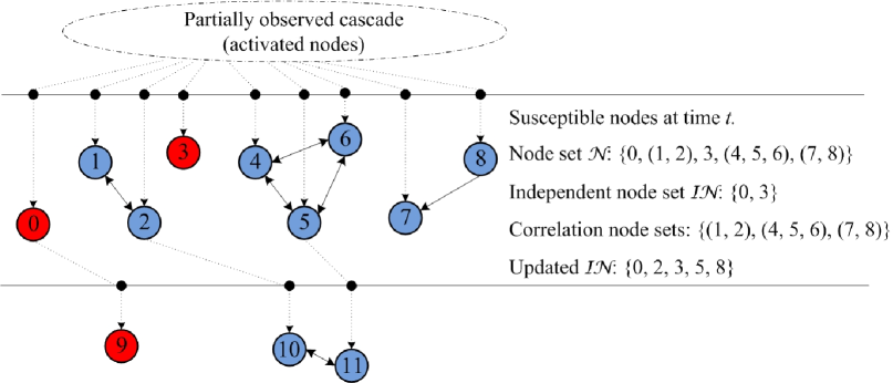
Figure 3: The local topology example of information cascades for FScaleADM. The topology contains two independent nodes and three correlation node sets. The updated independent node set contains the selected nodes from the correlation node sets after a random selection.

In FScaleADM, the susceptible nodes $\mathcal{N}$ at time $t$ can be viewed as a shell of the network. Ideally, the FScaleADM decomposes a network into hierarchically ordered shells by recursively activate the nodes with time stamps bigger than the ones of current shell. We denote the time increment between shells as $\Delta T$ in this paper. In reality, however, according to the discussion in the previous paragraph, all the susceptible nodes $\mathcal{N}$ in each shell are always cannot be updated and activated at one time but rather be updated on multiple independent node sets step by step. We define the time increment corresponding to the independent node sets $\mathcal{IN}$ as $\Delta t$, $\Delta t=|\mathcal{IN}|/|\mathcal{N}|\cdot\Delta T$. In this way, the spreading behaviors of the nodes in network shell are estimated asynchronously by asking all its neighbors’ labels. The overview of FScaleADM is presented in Algorithm 3.

Algorithm 3 FScaleADP Method

0:  (a) social network with partially observed cascade, (b) local spreading behavior estimation model $\mathcal{M}_{LBE}(G,C_{m}(t))=\{M,Fr,Fw\}$, (c) time increment $\Delta T$ and prediction time period $T$.

0:  Cascade condition after time period $T$.

1:  Get activation sequence $C_{m}$ and relevant time stamps $Ct_{m}$ from partially observed cascade

2:  Find the newest time stamp $t_{new}$ from $Ct_{m}$ and set $t\leftarrow t_{new}$.

3:  Compute susceptible nodes $\mathcal{N}$ based on activation sequence $C_{m}$ at current time.

4:  while $t<=t_{new}+T$ do

5:      (a) Get independent node set $\mathcal{IN}$ from susceptible nodes $\mathcal{N}$ with uniform probability..

6:      (b) Conduct $\mathcal{M}_{LBE}(G,C_{m}(t))$ on $\mathcal{IN}$ to update activation sequence $C_{m}$ and susceptible nodes $\mathcal{N}$.

7:      (c) Compute time increment: $\Delta t=|\mathcal{IN}|/|\mathcal{N}|\cdot\Delta T$.

8:      (d) Update system time: $t\leftarrow t+\Delta t$.

9:  end while

10:  Return the predicted cascade condition at time $t_{new}+T$ based on activation sequence $C_{m}$.

To illustrate FScaleADM Method, we will use a running example shown in Figure 4 to provide a demonstration. Initially, at time $t$, the susceptible node set $\mathcal{N}$ is {0, (1, 2), 3, (4, 5, 6), (7, 8)}, the independent node set $\mathcal{IN}$ is {0, 3} and correlation node sets are {(1, 2), (4, 5, 6), (7, 8)}. FSclaeADM selects nodes {2, 5, 8} from correlation node sets randomly and add them into independent node set $\mathcal{N}$. Then it estimates the spreading behaviors on the updated independent node set {0, 2, 3, 5, 8} with time increment ${5\mathord{\left/{\vphantom{5{9\cdot}}}\right.\kern-1.2pt}{9\cdot}}\Delta T$. Then it activates the nodes {0, 2, 3, 5} and updates the activated node set and susceptible node set. At time $t+{5\mathord{\left/{\vphantom{5{9\cdot}}}\right.\kern-1.2pt}{9\cdot}}\Delta T$, the susceptible node set $\mathcal{N}$ is {9, 1, (10, 11), (4, 6), (7, 8)}, the independent node set $\mathcal{IN}$ is {9, 1} and the updated independent node set $\mathcal{IN}$ is {9, 1, 10, 4, 8}. Then FSclaeADM activates the nodes {9, 1, 10, 8} with time increment ${5\mathord{\left/{\vphantom{5{8\cdot}}}\right.\kern-1.2pt}{8\cdot}}\Delta T$. In the same way, FSclaeADM updates nodes’ spreading behaviors iteratively in the later time.

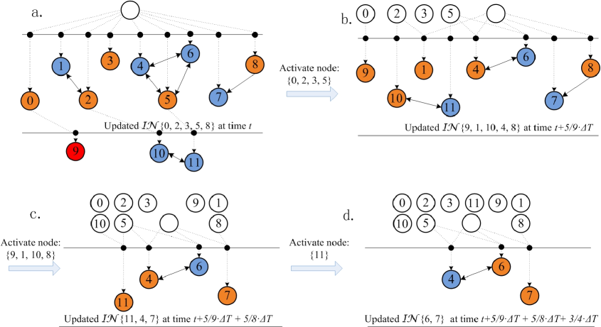
Figure 4: Illustrate of FScaleADP method. To the cascade conditions at different time, the nodes between two lines are the susceptible nodes at current time, in which the ones with white color are the activated nodes, the ones with orange color are the independent nodes, and the ones with blue color are the correlation nodes.

4.4 FScaleCP Properties

To prove the correctness and practicality of the FScaleCP framework, we prove by induction its properties.

Property 1 (Locality).

Given a graph $G$, a cascade activation sequence at time $t$ $C_{m}(t)$, then the information cascades prediction $FScaleCP(G,C_{m}(t))$ equals to conduct asynchronous diffusion process iteratively on the local topology of activated nodes, i.e. $FScaleCP(G,C_{m}(t))=FScaleADM(\mathcal{N}_{t},C_{m}(t))$, where $\mathcal{N}_{t}$ is the susceptible node set at time $t$.

As the messages propagate from activated nodes to inactivated nodes, at every point of time, the asynchronous diffusion process will merely be conducted on the topology region between the edge of the activated community and the inactivated neighbors.

Property 2 (Compositionality).

Given a graph $G$, a cascade activation sequence at time $t$ $C_{t}$ and the local topology of activated nodes. Since local topology’s bipartite graph structure, there always has much independent nodes. To independent node set $\mathcal{IN}$ in the local topology, consider any partition $\mathcal{IN}_{1}$, $\mathcal{IN}_{2}$, $...$, $\mathcal{IN}_{k}$ of the node set $\mathcal{IN}$, the asynchronous update process $FScaleADP(\mathcal{IN},C_{t})=FScaleADP(\mathcal{IN}_{1},C_{t})\cup FScaleADP(\mathcal{IN}_{2},C_{t})\cup...\cup FScaleADP(\mathcal{IN}_{k},C_{t})$.

This is a consequence of two facts: (1) Dividing the susceptible nodes into multiple independent partitions with few interaction is effortless, and (2) asynchronous diffusion process is conducted only on the local network topology of the activated nodes.

Property 3 (Convergence).

Given a graph $G$, a cascade activation sequence at time $t$ $C_{t}$, then the cascading process would converge if the local topology of activated users $G_{t}$ at multiple consecutive time point are same, i.e. $G_{t_{i}}=G_{t_{i+1}}=G_{t_{i+2}}$.

This is a consequence of the facts that each node has only two states about a cascade and node state is irreversible. That is, the cascading process is irreversible. So the convergence state must exist even if $V(G_{t})=\emptyset$.

Properties (1) and (2) have important computational repercussions. As the size of cascades grows, storing complete cascade graph may not be feasible. The locality property entails that FScaleCP can adapt to any information cascade. Moreover, the locality property and compositionality property entail that FScaleCP algorithm is highly parallelizable, because it can estimate the node behavior dynamics of different independent partitions simultaneously with relatively small combination work.

5 Experimental Results

In order to evaluate the performances and fully demonstrate the advantages of the proposed framework, we conduct a series of experiments on real-world data set, and the results of multiple tasks are reported.

5.1 Experimental Setup

Data Preparation. The social network we used in this study was crawled from Sina Weibo, which, similar to Twitter, is the largest microblogging network of china. The crawled way is illustrated in [26]. The data set includes 1.7 million users and 4 billion following relationships between them. For each user, the data set collects her 1000 most recent microblogs and all her profiles. In addition, the data set has 300000 microblog diffusion traces. We define the messages spreaded by user $v$ as positive training instances and the activated patents’ messages that are never been spreaded by node $v$ as negative training instances. As positive and negative instances are much unbalanced, we sample a balanced training data with equal number of positive and negative instances.

Comparison Methods. In order to show the efficiency of our proposed cascade prediction method, we compare the prediction results with the following baseline methods. First, we evaluate the performance on local spreading behavior estimation and e use LRC-Q1, LRC-Q2 as baselines. Then, since we are the first to investigate full-scale cascade dynamics prediction problem based on local behaviors estimation, no previous models can be adopted as direct baselines. Here, we use LRC-Q1, LRC-Q2 as the local spreading behavior estimation module of FScaleCP for full-scale cascade dynamics prediction evaluation. In addition, we implement the CG-CPred method as a baseline for final cascade size prediction evaluation.

FScaleCP with different feature sets. Comparing the performances of FScaleCP with different features sets will demonstrate the efficiency of the proposed local spreading behavior estimation model and the effectiveness of the optimal feature space. Meanwhile, comparing the performances of FScaleCP with different features sets can deepen the understanding about the effect of different driving mechanisms.

LRC-Q1. LRC-Q [26] is a typical implementation of individual spreading behavior estimation. In LRC-Q, the prediction task depends on a group of features from close friends in ego networks. LRC-Q measures pairwise influence using the theory of random walk with restart and structure influence by calculating the number of circles. LRC-Q trains logistic regression classifier for spreading behavior prediction. Let $S_{v}$ denote the collection of active neighbors in $v$’s ego network $G_{v}^{t}$ and $p_{v_{i}}$ denote the random walk probability from the active user $v_{i}$ to the given user $v$. Then the pairwise influence in LRC-Q1 is the sum of the random walk probabilities of all active neighbors, i.e.,

$$g(S_{v},G_{v}^{t})=\sum\limits_{v_{i}\in S_{v}}{p_{v_{i}}}$$ (8)

The structure influence in LRC-Q1 formulated by:

$$f(S_{v},G_{v}^{t})=e^{-\mu|C(S_{v})|}$$ (9)

where $C(S_{v})$ is the collection of circles formed by the active neighbors and $\mu$ is a decay factor.

LRC-Q2. Rather than using the definition of pairwise influence and structure influence in Eq. (8) and (9). LRC-Q2 consider the influence of time and the number of active neighbors, and it defines them as follows:

$$g(S_{v},G_{v}^{t})=\sum\limits_{v_{i}\in S_{v}}{h_{v_{i}}p_{v_{i}}}$$ (10)

$$f(S_{v},G_{v}^{t})=a\log(|S_{v}|+1)+be^{-\mu|C(S_{v})|}$$ (11)

where $h_{v_{i}}$ is the time difference and $a$ and $b$ are two balance parameters.

Cascade graph based cascade prediction (CG-CPred). To represent the methods utilizing the features generated from cascade graphs in early stage, we design cascade prediction approach CG-CPred capturing content semantic factors, temporal activity factors and the structural features of the cascade graphs in Sina Weibo scenario based on the method [14].

Evaluation Metrics. We perform 10-fold cross validation and evaluate the performance of different approaches in term of Precision (Prec.), Recall (Rec.), F1-measure (F1), and Accuracy(Acc.).

In our evaluation, we set the time increment $\Delta T$ to be five minutes and set the prediction period with different value according to prediction task. A large time increment $\Delta T$ may lead to network nodes miss the best spreading opportunity, and a small $\Delta T$ may bring too much spreading behavior estimation manipulations in the process of cascade dynamics prediction. So we set the value of $\Delta T$ according to people’s online behavior habits. Observe that a large number of microblogs are popular for only one day and a much large number of microblogs has never been popular. To the popular microblogs, the contagion rate slows down after two days when the microblogs have been published, and the contagion duration of most of them are in the range of five days.

5.2 Performance validation of FScaleCP

5.2.1 Behavioral Dynamics Estimation and Driving Mechanism Measure

Choice of Spreading Behavior Estimation Model. In this section, we consider the task of finding a suitable model for spreading behavior estimation. Based on all available features, we perform the classification task using a range of learning techniques, including Logistic Regression, Naive Bayes, SVM, Decision Tree and Random Forest. The results of them are summarized in Table 1. By comparing the accuracies of the linear and nonlinear methods, we can conclude that the training date is linear separable. Moreover, Table 1 presents that Random Forest obtains the best performance and Decision Tree gets the second-best performance in the spreading behavior estimation task. However, random Forests is more vulnerable to overfitting, hence, we select the Decision Tree classifier as FScaleCP’s spreading behavior estimation model. Except for Naive Bayes, the similar results of the other methods show that when sufficient information is available in features, the user identification task becomes reasonably accurate and is not very sensitive to the choice of learning algorithm.

Table 1: The performances of all candidate classifiers in spreading behavior estimation task.

Choice of Feature Space and Driving Mechanism Measure. To show the correctness of the candidate features, we analyze the effect of the features on the spreading behavior, and the results are shown in Figure 5. In Figure 5 (a), we classify thousands of messages according to their content length and count the number of the messages being spreaded in the past, and we plot the spreading probability of the messages under different content length. As the content length increases, the spreading probability grows slowly. In Figure 5 (b), we divide the data into four groups and find that the messages including keywords get higher spreading probability in all groups. Similarly, in Figure 5 (c), we can conclude that the spreading probability increases along with the interest diversity grows. Figure 5 (d) reports the average semantic similarity of positive instances and negative instances in five group data. We can find that positive instances have higher semantic similarity than negative ones. In the same way, we report the spreading probabilities under different average exposure time, average forwarding delay, average survival time of messages, candidate message number, social reinforcement and reciprocal active link proportion in Figure (e), (f), (g), (h). We observe that spreading probability is negatively correlated with average exposure time, average forwarding delay, average survival time of messages and candidate message number and positively correlated with social reinforcement and reciprocal active link proportion. The above results shows that the candidate features are effective in spreading behavior estimation respectively.

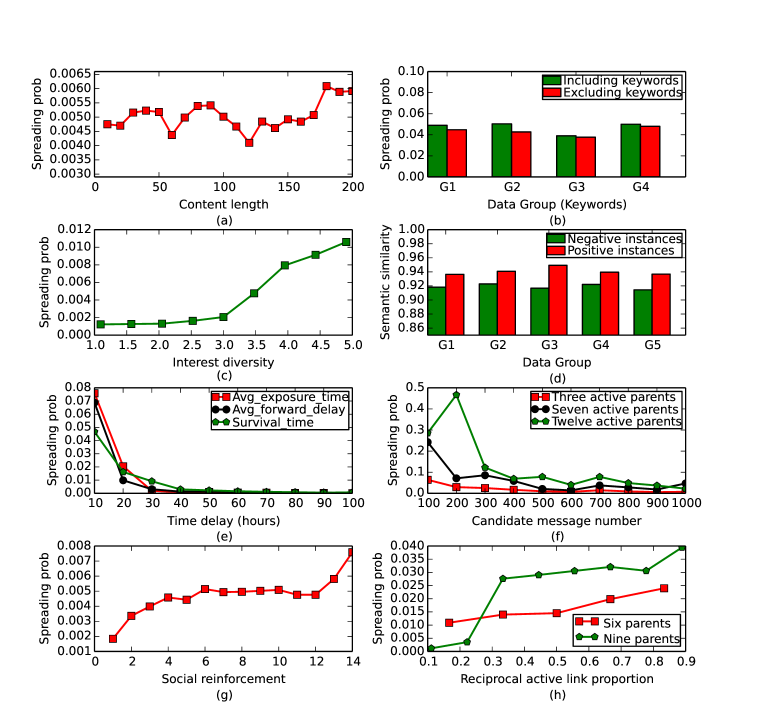
Figure 5: Features correctness analysis. (a) Spreading probability under different content length. (b) Influence of keywords on spreading probability. (c) Spreading probability under different interest diversity. (d) Semantic similarity of different instances. (e) Spreading probability under different time delay. (f) Influence of congnitive limitation on spreading probability. (g) Spreading probability under different social reinforcement. (h) Spreading probability under different reciprocal active link proportion.

Although all the candidate features are impactful in the task of spreading behavior estimation respectively, the predictive power of some of them is negligible and there may have correlation between them, which leads to unsatisfactory results and bad interpretability of estimation model. In order to distinguish the key factors from all the candidate features, we conduct the SFBS algorithm among them using Decision Tree classifier as criterion function and identify the optimal feature space from the 18-dimensional complete feature space. The result is shown in the second column of Table 2 (a) in descending order of weight.

Table 2: Feature evaluation and driving mechanism measure.

(a) Considering survival time

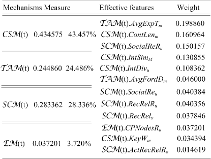
(a) Excluding survival time

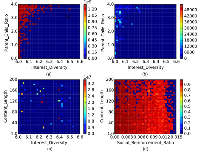
Figure 6: Features correlation analysis. (a) Heatmap of account creation time as a function of the ratio of child node number to parent node number and interest diversity, (b) Heatmap of related messages number as a function of the ratio of child node number to parent node number and interest diversity, (c) Heatmap of average exposure time as a function of content length and interest diversity, (d) Heatmap of semantic similarity as a function of content length and social reinforcement ratio.

According to Table 2 (a), the feature with the greatest weight is survival time $SurT_{m}$ of messages, which show that the most important factor for people in messages spreading is the novelty of messages. The next most effective feature is content length $ContLen_{m}$ of messages. Among the 13-dimensional optimal feature space, 4 features are elements of content semantic driving mechanism ${\mathcal{CSM}(t)}$, 3 features are elements of temporal activity driving mechanism ${\mathcal{TAM}(t)}$, 5 features are elements of surrounding conditions driving mechanism ${\mathcal{SCM}(t)}$ and 1 feature is element of endogenous driving mechanism $\mathcal{EM}(t)$. Based on the feature weights, the proportions of the driving mechanisms are 4.786%, 91.985%, 2.897% and 0.332% respectively. The result reveal a strong relationship between the ${\mathcal{TAM}(t)}$ and the spreading of messages. As the weight of feature $SurT_{m}$ is much larger than the others, we analyze the performance of the other features in detail to better understanding the driving mechanisms of information cascades, and the result is shown in Table 2 (b). We can find that the estimation accuracy decreases from 0.977449 to 0.864353, and the most important feature is the average exposure time $AvgExpT_{m}$ and the the most powerful driving mechanism is content semantic driving mechanism ${\mathcal{CSM}(t)}$.

Moverover, we explain the necessity of feature selection from correlation between features and spreading behavior estimation accuracy. As shown in Figure 6 (a), (b), the account creation time and related messages number have large values at the area of small interest diversity and large ratio of child node number to parent node number. Thus, the account creation time and related messages number can be expressed by the two features. Meanwhile, Figure 6 (c) show that average exposure time is not associated with content length and interest diversity. Similarly, Figure 6 (d) show that semantic similarity is not associated with content length and social reinforcement ratio. Thus, the fact that average exposure time and semantic similarity belong to the optimal feature space while account creation time and related messages number do not can as a exemplification to show that there have correlation between candidate features and FScaleCP can identify independent and effective features from them.

Spreading Behavior Estimation. Table 3 reports the estimation results by different methods using different features. From the table, we make the following observations. First, for FScaleCP method, the optimal features lead to the best accuracy and the complementary features generates the worst accuracy. The result shows that FScaleCP is effective in feature selection. Second, compared with LRC-Q1 and LRC-Q2, FScaleCP gets higher accuracy in spreading behavior estimation. The result demonstrates that FScaleCP has better performance than baseline methods. Third, compared with FScaleCP using all candidate features, the better accuracy of FScaleCP using optimal features shows that there may have conflict between multiple effective features and the estimation accuracy is not always increase along with the number of effective features.

Table 3: Spreading behavior estimation result using different features. OF: optimal features, AF: all candidate features, SF: structural features, UA: user attributes, CF: complementary features to OF.

5.2.2 Full-Scale Cascade Dynamics Prediction

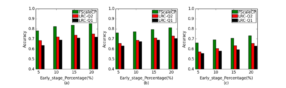
Figure 7: Contagion states prediction on cascades with different size. (a) Cascades with size at least 200. (b) Cascades with size at least 400. (c) Cascades with size at least 600.

Contagion States Prediction. We apply FScaleCP on cascades with different total size in five days and evaluation the performance of FSCaleCP by the activation accuracy obtained by averaging over 30 cascades in each group. The final results are shown in Figure 7. It can be seen that the methods generate different accuracy for varying sizes of believable activated nodes (from 5 percent to 20 percent) and the proposed method FScaleCP significantly outperforms other baselines in different sized cascades. We can see that the accuracy value grows along with the early stage percentage increases. Note that, the accuracy growth is not because the performance improvement of local spreading behavior estimation but because there are more activated nodes as believable information sources in cascade prediction. Moreover, the accuracy values decrease along with the size of cascades increases. The main reason is that a larger information cascade always presages a larger scope of information contagion and a larger number of hierarchical shells of the contagion network. The inaccuracy of local behavior estimations will be transmitted and amplified along with number of hierarchical shells increases.

Cascade Process Prediction. Except for the prediction of the final contagion state of network nodes, the prediction of contagion state at different time point of cascade processes is an important purpose of FScaleCP. We collect different sized cascades that are popular for only 2 days and predict the temporal contagion states with ten percent believable activated nodes at early stage. At every time point, the accuracies are computed based on all the contagion states of network nodes before current time. Then we average the prediction accuracies for all cascades and show the results in Figure 8. Here, we discover that FScaleCP always carries out the best performances in cascade process prediction. Moreover, the accuracies decrease with the prediction period increases. As local behavior estimation based FScaleCP is not directly related to prediction period, we argue that the declines in performance are mainly derived from the expansion of cascade ranges.

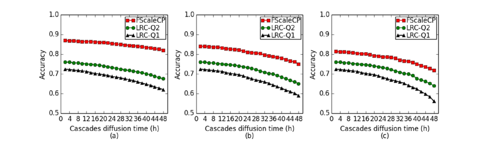
Figure 8: Cascade process prediction (i.e. temporal contagion states under different time point) on cascades with different size. (a) Cascades with size at least 200. (b) Cascades with size at least 400. (c) Cascades with size at least 600.

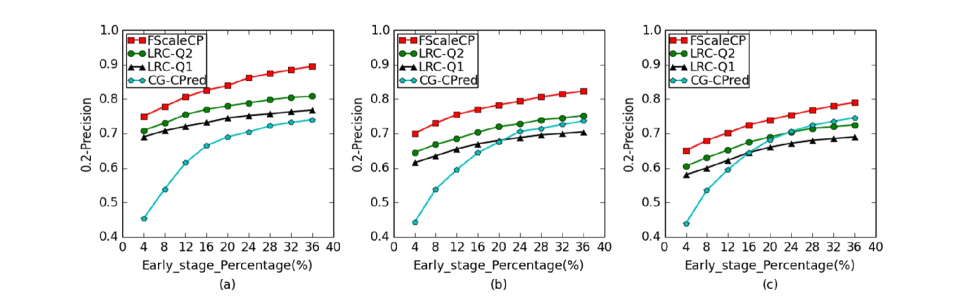
Figure 9: Cascade size prediction on cascades with different size. (a) Cascades with size at least 200. (b) Cascades with size at least 400. (c) Cascades with size at least 600.

Cascade Size Prediction. The final problem of this paper is to predict the final size of cascades. For example, in the early stage of a cascade, can we predict the final size of the cascade? We evaluate the prediction performance with different percentage of believable activated nodes in the cascades. In this case, we regard the predicted value within the range of groundtruth twenty percent as a correct prediction, and we use 0.2-Precision for result evaluation. As shown in Figure 9, the FScaleCP method gets the best performances on three groups of cascades in 0.2-Precision metric. Moreover, a clear advantage of FScaleCP over traditional methods is that FScaleCP is not dependent on the large percentage of early stage, although it can improve FScaleCP’s performance. We can see that the precision of CG-CPred is unsatisfactory when only a small percent of observed nodes available.

Compared with the traditional methods, the proposed method can predict when and which nodes will be activated and is not dependent on the percentage of observed nodes. However, we recognize that our approach has prediction limitations in networks with large number of hierarchical structure shells. To these networks, excellent performance can be generated when multiple information sources are scattered in networks.

5.3 Complexity Analysis

At every update period, the local spreading behavior estimation model $\mathcal{M}_{LBE}(G,C_{m}(t))=\{M,Fr,Fw\}$ is conducted on the nodes in independent node set $\mathcal{IN}$. The time complexity is $O(|\mathcal{IN}|)$, where $|\mathcal{IN}|$ is the size of the node set. To estimate the local spreading behaviors of each node, the feature information of training instances is required. Thus the time computation becomes $O(k\cdot|\mathcal{IN}|)$, where $k$ is the number of features. During the diffusion process in prediction period $T$, all independent node sets need to be checked to estimate their nodes’ spreading behaviors, the approximate total check number is $T/\Delta t$, where $\Delta t$ is the time increment corresponding to each independent node set. Thus the time complexity is $O(k\cdot|\mathcal{IN}|\cdot T/\Delta t)$. With the time increment $\Delta T$ between susceptible node shells to express $\Delta t$, $\Delta t=|\mathcal{IN}|/|\mathcal{N}|\cdot\Delta T$, the time complexity can be rewritten as $O(k\cdot|\mathcal{IN}|\cdot T/(|\mathcal{IN}|/|\mathcal{N}|\cdot\Delta T))$ = $O(k\cdot|\mathcal{N}|\cdot T/\Delta T)$. Note that, $|\mathcal{N}|$ is not constant, and it varies along with the diffusion process.

6 Discussion and Conclusion

Cascades prediction has always been an important research topic. Though many related researches have been done, most of them focus only on indicator features exploration and final size prediction, and little has been down in problem of investigating cascade dynamics comprehensively. In this paper, we have proposed a local-first cascade dynamics prediction framework FScaleCP. The proposed framework can predict cascade dynamics and is dependent of the cascade graph in early stage. Moreover, FScaleCP is not only predicting the final size of cascades, but also when and which nodes will be activated. By the driving mechanisms measure, FScaleCP identifies the most cardinal influencing factors and deepens the understanding about cascade dynamics. The results would provide basis for cascades control and theoretical modeling of information cascades. Finally, experiments results show that the proposed FScaleCP perform better than baseline methods.

Overall, FScaleCP is a practical yet general approach since it mainly focuses on modeling the cascade dynamics. In this paper, we just simply explore some basis influencing factors as features, other various factors can be integrated into the framework conveniently. Moveover, we assume that the network structure is static in cascade process. However, the real-world network structure varies along with the social interaction between uses. Therefore, it is necessary to understand cascade dynamics using dynamic social networks.

References

References

- [1] Weng, L., Menczer, F., Ahn, Y. Y. (2013). Virality prediction and community structure in social networks. Scientific reports, 3.
- [2] Cui, P., Tang, M., Wu, Z. X. (2014). Message spreading in networks with stickiness and persistence: Large clustering does not always facilitate large-scale diffusion. Scientific reports, 4.
- [3] Guille, A., Hacid, H., Favre, C., Zighed, D. A. (2013). Information diffusion in online social networks: A survey. ACM SIGMOD Record, 42(2), 17-28.
- [4] Romero, D. M., Meeder, B., Kleinberg, J. (2011, March). Differences in the mechanics of information diffusion across topics: idioms, political hashtags, and complex contagion on twitter. In Proceedings of the 20th international conference on World wide web (pp. 695-704). ACM.
- [5] Wu, S., Hofman, J. M., Mason, W. A., Watts, D. J. (2011, March). Who says what to whom on twitter. In Proceedings of the 20th international conference on World wide web (pp. 705-714). ACM.
- [6] Rodriguez, M. G., Balduzzi, D., Scholkopf, B. (2011). Uncovering the temporal dynamics of diffusion networks. arXiv preprint arXiv:1105.0697.
- [7] Farajtabar, M., Gomez-Rodriguez, M., Wang, Y., Li, S., Zha, H., Song, L. (2015, May). Co-evolutionary Dynamics of Information Diffusion and Network Structure. In Proceedings of the 24th International Conference on World Wide Web Companion (pp. 619-620). International World Wide Web Conferences Steering Committee.
- [8] Yu, L., Cui, P., Wang, F., Song, C., Yang, S. (2015). From Micro to Macro: Uncovering and Predicting Information Cascading Process with Behavioral Dynamics. arXiv preprint arXiv:1505.07193.
- [9] Weng, L., Menczer, F., Ahn, Y. Y. (2014). Predicting successful memes using network and community structure. arXiv preprint arXiv:1403.6199.
- [10] Ma, Z., Sun, A., Cong, G. (2013). On predicting the popularity of newly emerging hashtags in twitter. Journal of the American Society for Information Science and Technology, 64(7), 1399-1410.
- [11] Hong, L., Dan, O., Davison, B. D. (2011, March). Predicting popular messages in twitter. In Proceedings of the 20th international conference companion on World wide web (pp. 57-58). ACM.
- [12] Kupavskii, A., Ostroumova, L., Umnov, A., Usachev, S., Serdyukov, P., Gusev, G., Kustarev, A. (2012, October). Prediction of retweet cascade size over time. In Proceedings of the 21st ACM international conference on Information and knowledge management (pp. 2335-2338). ACM.
- [13] Tsur, O., Rappoport, A. (2012, February). What’s in a hashtag?: content based prediction of the spread of ideas in microblogging communities. InProceedings of the fifth ACM international conference on Web search and data mining (pp. 643-652). ACM.
- [14] Cheng, J., Adamic, L., Dow, P. A., Kleinberg, J. M., Leskovec, J. (2014, April). Can cascades be predicted?. In Proceedings of the 23rd international conference on World wide web (pp. 925-936). ACM.
- [15] Wu, T., Guo, Y., Chen, L., Liu, Y. (2015). Integrated structure investigation in complex networks by label propagation. 10.1016/j.physa.2015.12.073.
- [16] Anagnostopoulos, A., Kumar, R., Mahdian, M. (2008, August). Influence and correlation in social networks. In Proceedings of the 14th ACM SIGKDD international conference on Knowledge discovery and data mining (pp. 7-15). ACM.
- [17] Crandall, D., Cosley, D., Huttenlocher, D., Kleinberg, J., Suri, S. (2008, August). Feedback effects between similarity and social influence in online communities. In Proceedings of the 14th ACM SIGKDD international conference on Knowledge discovery and data mining (pp. 160-168). ACM.
- [18] Aral, S., Muchnik, L., Sundararajan, A. (2009). Distinguishing influence-based contagion from homophily-driven diffusion in dynamic networks.Proceedings of the National Academy of Sciences, 106(51), 21544-21549.
- [19] Goyal, A., Bonchi, F., Lakshmanan, L. V. (2010, February). Learning influence probabilities in social networks. In Proceedings of the third ACM international conference on Web search and data mining (pp. 241-250). ACM.
- [20] Tang, J., Sun, J., Wang, C., Yang, Z. (2009, June). Social influence analysis in large-scale networks. In Proceedings of the 15th ACM SIGKDD international conference on Knowledge discovery and data mining (pp. 807-816). ACM.
- [21] Wu, F., Huberman, B. A. (2007). Novelty and collective attention.Proceedings of the National Academy of Sciences, 104(45), 17599-17601.
- [22] Cui, P., Tang, M., Wu, Z. X. (2014). Message spreading in networks with stickiness and persistence: Large clustering does not always facilitate large-scale diffusion. Scientific reports, 4.
- [23] Bao, P., Shen, H. W., Chen, W., Cheng, X. Q. (2013). Cumulative effect in information diffusion: empirical study on a microblogging network. PloS one, 8(10), e76027.
- [24] Weng, L., Flammini, A., Vespignani, A., Menczer, F. (2012). Competition among memes in a world with limited attention. Scientific reports, 2.
- [25] Hodas, N. O., Lerman, K. (2014). The simple rules of social contagion.Scientific reports, 4.
- [26] Zhang, J., Liu, B., Tang, J., Chen, T., Li, J. (2013, August). Social influence locality for modeling retweeting behaviors. In Proceedings of the Twenty-Third international joint conference on Artificial Intelligence (pp. 2761-2767). AAAI Press.
- [27] Blei, D. M., Ng, A. Y., Jordan, M. I. (2003). Latent dirichlet allocation. the
- [28] Pudil, P., Novovi?ov , J., Kittler, J. (1994). Floating search methods in feature selection. Pattern recognition letters, 15(11), 1119-1125.