An optimisation approach for fuel treatment planning to break the connectivity of high-risk regions

Abstract

Uncontrolled wildfires can lead to loss of life and property and destruction of natural resources. At the same time, fire plays a vital role in restoring ecological balance in many ecosystems. Fuel management, or treatment planning by way of planned burning, is an important tool used in many countries where fire is a major ecosystem process. In this paper, we propose an approach to reduce the spatial connectivity of fuel hazards while still considering the ecological fire requirements of the ecosystem. A mixed integer programming (MIP) model is formulated in such a way that it breaks the connectivity of high-risk regions as a means to reduce fuel hazards in the landscape. This multi-period model tracks the age of each vegetation type and determines the optimal time and locations to conduct fuel treatments. The minimum and maximum Tolerable Fire Intervals (TFI), which define the ages at which certain vegetation type can be treated for ecological reasons, are taken into account by the model. Previous work has been limited to using single vegetation types implemented within rectangular grids. In this paper, we significantly extend previous work by modelling multiple vegetation types implemented within a polygon-based network. Thereby a more realistic representation of the landscape is achieved. An analysis of the proposed approach was conducted for a fuel treatment area comprising 711 treatment units in the Barwon-Otway district of Victoria, Australia. The solution of the proposed model can be obtained for 20-year fuel treatment planning within a reasonable computation time of eight hours.

1 Introduction

Uncontrolled wildfires can result in the loss of life and economic assets and the destruction of natural resources (King et al., 2008). Southern Australia, Mediterranean Europe and areas of the United States are among the top regions in the world that are affected by frequent wildfires (Bradstock et al., 2012). Coupled with the proximity of major cities to natural ecosystems prone to wildfire, the management of fuel hazard becomes an important land management policy and planning issue for the protection of human life and assets (Collins et al., 2010). However, it is also acknowledged that fuel management for asset protection cannot be done in isolation of the ecological requirements of the ecosystem. Maintaining the ecological integrity of the landscape must also be considered (Penman et al., 2011).

Fuel management is a method to modify the structure and amount of fuel. The methods include prescribed burning and mechanical clearing (King et al., 2008; Loehle, 2004). Fuel management programs have been extensively implemented in the USA (Ager et al., 2010; Collins et al., 2010) and Australia (Boer et al., 2009; McCaw, 2013) in an effort to lessen the risk posed by wildfire. The choice of fuel treatment location plays a substantial role in conducting efficient fuel treatment scheduling (Collins et al., 2010). Instead of randomly selecting the locations, significantly better protection in a landscape could be provided by a fuel treatment schedule that takes into account the relationships between treatment units (Schmidt et al., 2008). Research indicates that it is important to choose where to conduct the fuel treatment by considering spatial arrangement (Rytwinski and Crowe, 2010; Kim et al., 2009; Chung, 2015). The importance of landscape-level fuel treatment has been observed in a number of studies. In wilderness regions in the United States, a mosaic of varying fuel ages is formed as a result of free burning fires. A particular arrangement of old and new treatment units has been recognised to delay large wildfires in the following year (Finney, 2007). Research conducted in the Sierra Nevada forests of the United States has shown that wildfire size can be modified by spatial fragmentation of fuel (Van Wagtendonk, 1995). Prescribed burning has been implemented in the eucalypt forests in south-western Australia over the past 50 years. The connectivity of ‘old’ untreated patches has been revealed to be the main aspect that contributes to wildfire extent (Boer et al., 2009).

Previous studies have proposed mathematically modelling fuel treatment schedules methods for reducing fuel hazards. The studies had different objective functions and took into account various considerations in building up the models. Ferreira et al. (2011) propose a stochastic dynamic programming (SDP) approach to determine the fuel treatment scheduling that produces the maximum expected discounted net revenue while mitigating the risk of fire. The method was then applied to a maritime pine forest in Leiria National Forest, Portugal. They found that the approach was efficient and can efficiently help integrating wildfire risk in stand management planning. Garcia-Gonzalo et al. (2011) use the Hooke-Jeeves direct search method to determine the optimal fuel treatment scheduling for reducing expected damage and increasing the revenue to the same landscape, as that of Ferreira et al. (2011). Their research shows that the fuel treatments improve productivity as well as reduce the potential damage. Rachmawati et al. (2015) propose a model that can lessen the risk of fire by reducing the total fuel load but do not consider spatial properties or the spatial relationship between the treatment units. Wei and Long (2014) propose a single-period model to fragment high-risk patches by considering future fire spread speeds and durations. Minas et al. (2014) propose a model that breaks the connectivity of high fuel units in the landscape to prevent the fires spreading. The model proposed by Minas et al. (2014) takes into account vegetation dynamics in the landscape, but this is limited to a simplistic grid representation of a single vegetation type per treatment unit. In reality, a treatment unit may comprise a number of patches with different vegetation type and age. In summary, most of the models reviewed can be improved by taking into account multi-vegetation types and ages within a treatment unit and using a polygon-based network representation.

In this paper, we build upon previous work by incorporating multiple vegetation types found in the landscape and within single treatment units, and take into account the spatial connectivity or fragmentation of ‘high-risk’ treatment units. We also use a more realistic polygon-based network representation of the landscape to better capture the spatial complexity of this problem rather than a rectangular grid. Besides the negative impacts of wildfires, the role of fire in ecology has been widely acknowledged. Fire is required to maintain a healthy ecosystem and it also has a significant role in habitat regeneration. Many vegetation species in fire-adapted ecosystems need fire to reproduce. For instance, germination of seeds and successful establishment of plants in the jarrah forests of Western Australia is very rarely found without fire intervention (Burrows and Wardell-Johnson, 2003). More recently, Burrows (2008) argues that fuel management is important to support biodiversity conservation as well as to reduce the negative impact of wildfires. A recognition of vegetation dynamics over time is crucial in the planning of fuel treatment (Krivtsov et al., 2009). In this proposed model, the ecological fire requirements of each vegetation type can be described using the minimum and maximum Tolerable Fire Intervals (TFI). The minimum TFI is the minimum time required between two consecutive fire events at a location and is based on the time to reach maturity of the sensitive species in the vegetation class. The maximum TFI refers to the maximum time needed between two fire events at a location that considers the fire interval required for fire-adapted species rejuvenation (Cheal, 2010). In this paper, we assume that treating of vegetation whose age is between these two intervals will maintain species diversity and hence support the ecosystem’s health. Therefore, we select not to treat a treatment unit if the age of vegetation growing in that location is under the minimum TFI. In contrast, treatment units with vegetation over the maximum TFI must be treated. In this paper, we assume that the high-risk threshold age is between these two intervals. The objective of the model proposed in this paper is to reduce the spatial connectivity of fuel hazards while still considering the fire requirements of the ecosystem. The question that then arises is when and where to conduct fuel treatment to meet this objective, that can be solved for spatially complex landscapes with long planning horizons?

A Mixed Integer Programming (MIP) model is proposed for multi-period fuel treatment scheduling. The model tracks the vegetation age in each treatment unit yearly for both treated and untreated areas. The model is then applied to a real landscape in southern Australia that comprises different shapes and sizes of treatment units.

2 Problem formulation

In this section, we explain the terms ‘treatment unit’ and ‘patch’ that we use to formulate the problem. The candidate locations for fuel treatment are represented by treatment units. A treatment unit comprises multiple patches. Each vegetation type growing in a treatment unit is represented by a patch and within each patch all the vegetation is of the same age. The data in each patch includes area, vegetation type and age. Patches within a single treatment unit may have different vegetation type and age, defining a ‘multi-vegetation treatment unit’.

Each vegetation type has a ‘high risk’ age threshold. For example, grass and bush are considered to be high risk when they reach four and seven years old, respectively. Since we know the vegetation type and age in each patch, we then know whether a patch is a high-risk patch or not at any given time. In order to disconnect the high-risk treatment units in a landscape, we need a method to determine whether a treatment unit is a high-risk treatment unit or not. In this paper, we assume that if ignitions occur, the fires will likely spread through connected high-risk treatment units. From this, we believe that if we can disconnect high-risk treatments unit as much as possible, the possibility of catastrophic fires can be reduced.

Each treatment unit selected for fuel treatment should not violate the ecological requirements. Each vegetation type has its specific minimum and maximum TFI. We assume that a healthier ecosystem can be maintained when the fuel treatment is conducted when the vegetation age is between the minimum and the maximum TFI.

3 Model formulation

The model is formulated to determine when and where to conduct the fuel treatment each year to break the connectivity of high-risk treatment units and to meet the ecological requirements. We consider a landscape divided into treatment units where each treatment unit might consist of multiple patches. The following mixed integer programming model is formulated.

Sets:

$C$ is the set of all treatment units in the landscape

$\Psi\subset C$ is the set of treatment units where fuel treatment is not permitted

$\varLambda\subset C$ is the set of treatment units where fuel treatment is permitted (where $\varLambda=C-\Psi$)

$P_{i}$ is the set of patches in treatment unit $i$

$\varPhi_{i}$ is the set of treatment units connected to treatment unit $i$

$T$ is the planning horizon

Indices:

$p$ = patch

$i$ = treatment unit

$t$ = period, $t$ = 0, 1, 2, …T

Parameters:

$w_{i,j}$ = relative importance (weight) of connectivity of treatment units i and j

$a_{p}$ = initial vegetation age in patch p

$Area_{p}$= area of patch p

$\rho$ = treatment level (in percentage), i.e. the maximum proportion of the total area

that fuel treatment is permitted in a landscape selected for treatment

$R$ = the total area of treatment units in the landscape where fuel treatment is permitted

$c_{i}$= area of treatment unit $i$

$d_{p}$ = high-risk age threshold for patch p, based upon the vegetation type growing

in that patch

$maxTFI_{p}$= maximum tolerable fire interval (TFI) of vegetation type growing in patch $p$

$minTFI_{p}$ = minimum TFI of vegetation type growing in patch $p$

$H$ = the threshold for the area proportion of the high-risk patches in a treatment unit

to be a high-risk treatment units

Decision variables:

$A_{p,t}$ = vegetation age in patch p at time t

$x_{i,t}=\begin{cases}1&\mbox{if treatment unit \emph{i} is treated in time period \emph{t}}\\ 0&\mbox{otherwise}\end{cases}$

$Riskpatch_{p,t}=\begin{cases}1&\mbox{if patch \emph{p} is classified as high-risk patch in time period \emph{t}}\\ 0&\mbox{otherwise}\end{cases}$

$Risk_{i,t}=\begin{cases}1&\mbox{if treatment unit \emph{i} is classified as high-risk treatment unit in time period \emph{t}}\\ 0&\mbox{otherwise}\end{cases}$

$RiskConn_{i,j,t}=\begin{cases}1&\mbox{if connected treatment units \emph{i} and \emph{j} are both high-risk treatment units in time period \emph{t}}\\ 0&\mbox{otherwise}\end{cases}$

$Old_{p,t}=\begin{cases}1&\textrm{if patch \emph{p }is classified as\text{ \textquoteleft}old\text{\textquoteright\ }(over-the-maximum-TFI)}\\ &\textrm{patch in time period \emph{t}}\\ 0&\textrm{otherwise}\end{cases}$

$Young_{p,t}=\begin{cases}1&\textrm{if patch \emph{p }is classified as\text{ \textquoteleft}young\text{\textquoteright\ }(under-the-minimum-TFI)}\\ &\textrm{patch in time period \emph{t}}\\ 0&\textrm{otherwise}\end{cases}$

Minimise the weighted connectivity of high-risk treatment units

$$z=\underset{t=1}{\overset{T}{\sum}}\underset{i\in C}{\sum}\underset{j\in\varPhi_{i},i<j}{\sum}w_{i,j}RiskConn_{i,j,t}$$ (1)

subject to

$$\underset{i}{\sum}c_{i}x_{i,t}\leq\rho R,\;t=1\ldots T,\forall i\in\varLambda$$ (2)

$$A_{p,0}=a_{p},\;\forall p$$ (3)

$$A_{p,t}=A_{p,t-1}+1,\;\forall p\in P_{i},t=1\ldots T,\forall i\in\varPsi$$ (4)

$$A_{p,t}\geq A_{p,t-1}+1-M_{1}x_{i,t},\;\forall p\in P_{i},t=1\ldots T,\forall i\in\varLambda$$ (5)

$$A_{p,t}\leq M_{2}(1-x_{i,t}),\;\forall p\in P_{i},t=1\ldots T,\forall i\in\varLambda$$ (6)

$$A_{p,t}\leq A_{p,t-1}+1,\;\forall p\in P_{i},t=1\ldots T,\forall i\in\varLambda$$ (7)

$$A_{p,t}-d_{p}\leq M_{3}Riskpatch_{p,t}-1,\;\forall p\in P_{i},t=1\ldots T,\forall i\in C$$ (8)

$$\underset{p\in P_{i}}{\overset{}{\sum}}Area_{p}Riskpatch_{p,t}-H\underset{p\in P_{i}}{\overset{}{\sum}}Area_{p}\leq M_{4}Risk_{i,t},\;t=1\ldots T,\forall p\in P_{i},\forall i\in C$$ (9)

$$Risk_{i,t}+Risk_{j,t}-RiskConn_{i,j,t}\leq 1,\;t=1\ldots T,\forall j\in\varPhi_{i},i<j,\forall i\in C$$ (10)

$$A_{p,t}-maxTFI_{p}\leq M_{5}Old_{p,t}-1,\;\forall p\in P_{i},t=0\ldots T-1,\forall i\in\varLambda$$ (11)

$$A_{p,t}\geq maxTFI_{p}Old_{p,t},\;\forall p\in P_{i},t=0\ldots T-1,\forall i\in\varLambda$$ (12)

$$A_{p,t}+M_{6}Young_{p,t}\geq minTFI_{p},\;\forall p\in P_{i},t=0\ldots T-1,\forall i\in\varLambda$$ (13)

$$A_{p,t}-M_{7}(1-Young_{p,t})\leq minTFI_{p}-1,\;\forall p\in P_{i},t=0\ldots T-1,\forall i\in\varLambda$$ (14)

$$Young{}_{p,t-1}\leq 1-x{}_{i,t},\;t=1\ldots T,\forall i\in\varLambda$$ (15)

$$\underset{p\in P_{i}}{\sum}Old{}_{p,t-1}-\mid V_{i}\mid\underset{p\in P_{i}}{\sum}Young{}_{p,t-1}\leq\mid V_{i}\mid x_{i,t},\;t=1\ldots T,\forall i\in\varLambda$$ (16)

$$x_{i,t},\;Riskpatch_{p,t},\;Risk_{i,t},\;RiskConn_{i,j,t},\;Young_{p,t},\;Old_{p,t}\in\{0,1\}$$ (17)

The objective function (1) minimises the weighted connectivity of high-risk treatment units in a landscape throughout a planning horizon.

Constraint (2) specifies that the total area selected for fuel treatment annually is not more than the area allotted (target) each year for fuel treatment (in hectares).

Constraint (3) sets the initial vegetation age in a patch. Constraint (4) to (6) track the vegetation age of each patch. Constraint (4) relates to the set of treatment units where fuel treatment is not permitted. Constraint (5) and (6) indicate that when $x_{i,t}=0$, the vegetation in that area will continue growing until the following period, and the age will be incremented by one. Whereas if $x_{i,t}=1$, the vegetation age will reset to zero. Constraint (7) increments vegetation age by exactly one year if the treatment unit is not treated.

Constraint (8) uses binary variable $Riskpatch_{p,t}$ to classify a patch to be a high-risk patch if the vegetation age in that patch reaches or exceeds a threshold value, thus each patch has its own age threshold. Then, within a single treatment unit, we can compare the area of over-the-threshold patch. Here, we define a treatment unit is a high-risk treatment unit if the proportion of the over the threshold area is greater than a certain proportion of the total treatable area of the treatment unit. Constraint (9) represents this requirement. In constraint (10), $RiskConn_{i,j,t}$ takes the value one if connected treatment units i and j are both classified as high-risk treatment units in time period t .

Constraints (11) to (14) classify a patch to be an ‘old’ or a ‘young’ patch based on TFI values. Constraint (15) ensures that the treatment units containing young patches cannot be treated. Constraint (16) states that if there is at least one patch within a treatment unit is ‘old’ and no young patch, then the treatment unit must be treated. Here, $|V_{i}|$ represents the number of patches in treatment unit $i$. This constraint avoids a deadlock that may occur when a treatment unit consists of a young and an old patch at the same time. In this study, we break the deadlock in favour of young patch.

Constraints (17) ensures that the decision variables take binary values.

3.1 Model improvements

The solution time can be improved by reducing the number of variables. As discussed earlier, the initial age of each vegetation type in each treatment unit is given. We also assume that the age of vegetation type growing in the treatment units where fuel treatment is not permitted should always be incremented by one. For this reason, we no longer need constraint (4) to track the vegetation in the area. The time for the vegetation type to reach the high-risk age threshold can be determined. And because we assume that we cannot treat the treatment units, once the vegetation type hits the threshold it will remain high risk. Therefore, within a planning horizon we can determine whether a treatment unit is high risk or not.

Decision variables $A_{p,t}$ and $Riskpatch_{p,t}$ for the treatment units where fuel treatment is not permitted can be omitted, and regarded as parameters instead. This results in a faster solution time.

We can rewrite our model as follows. Constraint (4) is excluded, because at any given time the age of vegetation growing in the treatment units where fuel treatment is not permitted is known. Constraints (8) and (9) are only defined for treatable treatment units. All other constraints remain the same. However, we introduce these two constraints to the model for the treatment units where fuel treatments are not permitted:

$$Risk_{i,t}=0,\>\forall t\>\textrm{when}\>\theta\leq 0,\forall i\in\Psi$$ (18)

$$Risk_{i,t}=1,\>\forall t\>\textrm{when}\>\theta>0,\forall i\in\Psi$$ (19)

where $\theta=\underset{p\in P_{i}}{\overset{}{\sum}}Area_{p}Riskpatch_{p,t}-H\underset{p\in P_{i}}{\overset{}{\sum}}Area_{p}$

In constraint (18), value 0 is assigned to $Risk_{i,t}$ if less than a certain proportion of the total treatable area of the treatment unit is high risk at time t. And in constraint (19) value 1 is assigned to $Risk_{i,t}$ if more than a certain proportion of the total treatable area of the treatment unit is high risk at time t.

4 Implementation of the new approach

Initially, it may not be possible to treat all treatment units according to the maximum TFI value because of the annual limit, $\rho$. This maximum TFI requirement may lead to the infeasibility of the initial problem. In order to bring the system under control and to avoid the initial infeasibility, we propose a preliminary stage, namely Phase 1. From the initial data, we can identify treatment units containing an old patch or would potentially be containing an old patch in the following year and have no young patches. We are trying to eliminate the treatment units containing old patches to ensure feasibility. In this phase, we exclude the TFI constraints, which are constraints (11) to (16). We run the model without enforcing the constraint ensuring treatment of old patches for some years, and modify the objective function as follows:

maximise

$$z=\underset{t=1}{\overset{N}{\sum}}\underset{i\in\varTheta}{\sum}c_{i}x_{i,t}-\underset{t=1}{\overset{N}{\sum}}\underset{i\in\varTheta}{\sum}\underset{j\in\varPhi_{i},i<j}{\sum}\varepsilon_{i}RiskConn_{i,j,t}$$ (20)

where $\varTheta$ is the set of treatment units that contains an old patch or potentially contains an old patch in the following year and no young patch. $\varepsilon_{i}$ is a relatively small number ($\varepsilon_{i}\ll c_{i}$) representing the weight of connectivity of treatment unit $i$. N is the planning horizon.

The objective is to maximise the area treated and to minimise the weighted connectivity of the treatment units in a landscape for a number of years ahead. The planning horizon (N) increased incrementally until the initial problem is feasible.

For the landscape that comprises mostly old treatment units, the solution from this phase becomes the input for Phase 2. In Phase 2, the model presented in Section 3 is run.

5 Model demonstration

For the model demonstration, consider a test landscape comprising 29 treatment units that are a subset of the case study in the Barwon-Otway district of Victoria, Australia. Figure 1a represents the map of the landscape and Figure 1b illustrates the graph representing the neighbourhood of each treatment unit. We assume that two treatment units are neighbouring if they have common boundaries. Table 1 represents data for each Ecological Vegetation Class (EVC) and the associated threshold age, the minimum and the maximum TFI for this test landscape. The data regarding the area of the treatment units, vegetation type (EVC) and age can be seen in Table 2.

Figure 1: A landscape for the model demonstration (29 treatment units)

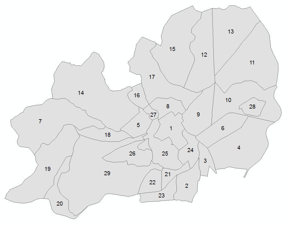
(a) Map of the landscape

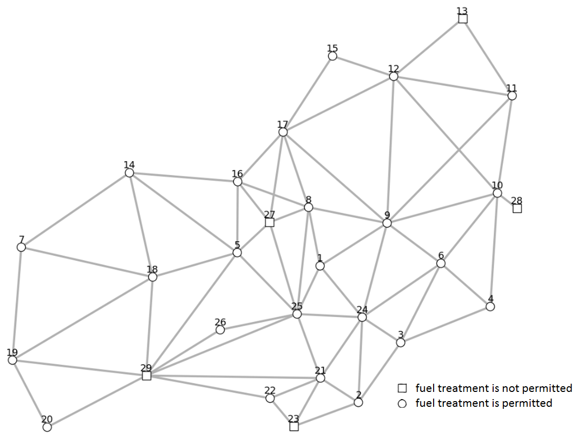
(b) The neighbourhood graph of the landscape

Table 1: Ecological Vegetation Class (EVC) and the associated threshold age, the minimum and the maximum TFI for the test landscape

EVC code	min TFI (year)	max TFI (year)	threshold (year)
1	3	10	5
3	4	15	7
6	7	20	10

Table 2: 29 treatment units data containing vegetation type, extent and age

Treatment unit ID	EVC code	area (ha)	age (years)		7	6	34	11		18	6	10	9
1	1	10	6		8	1	19	5		19	1	50	5
1	3	8	7		8	3	12	7		19	3	37	5
1	6	14	11		9	1	46	4		20	1	10	1
2	1	10	5		10	1	78	6		20	3	6	2
2	3	21	8		11	1	30	4		20	6	14	10
3	1	4	1		11	3	50	8		21	1	5	1
3	3	5	1		11	6	30	12		21	3	8	1
3	6	7	1		12	1	40	5		22	3	19	7
4	1	40	5		12	3	34	7		23	6	20	11
4	3	30	6		13	6	84	11		24	6	22	10
4	6	24	10		14	3	80	7		25	1	42	1
5	1	8	1		14	6	76	11		26	3	33	7
5	3	10	1		15	6	103	12		27	3	6	6
5	6	4	1		16	3	14	5		28	1	14	5
6	1	18	1		17	1	50	5		29	1	100	5
6	3	20	1		17	3	32	6		29	3	50	6
7	3	80	8		18	3	14	5		29	6	41	9

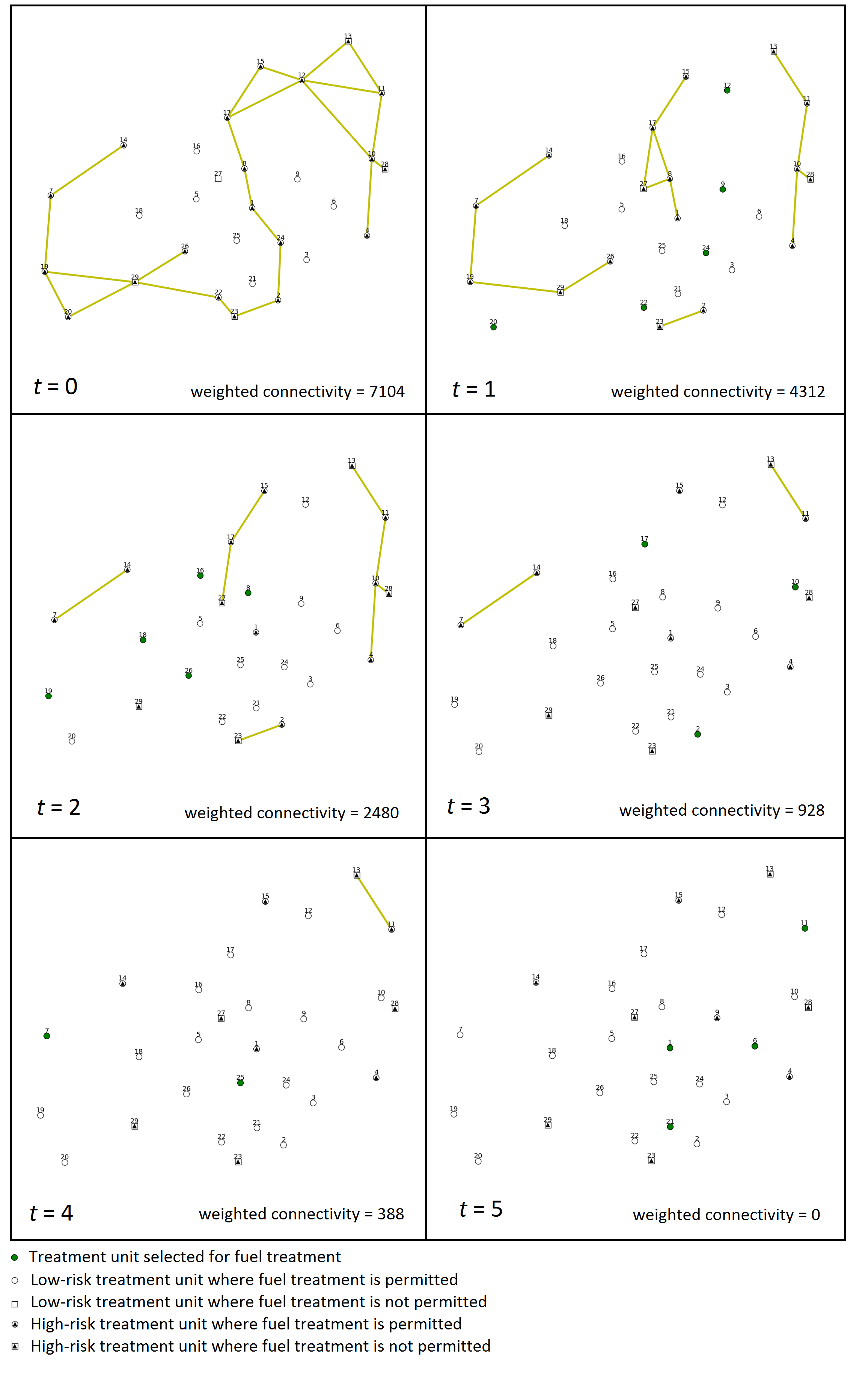
Figure 2: A network represents the fuel treatment schedule for the test landscape

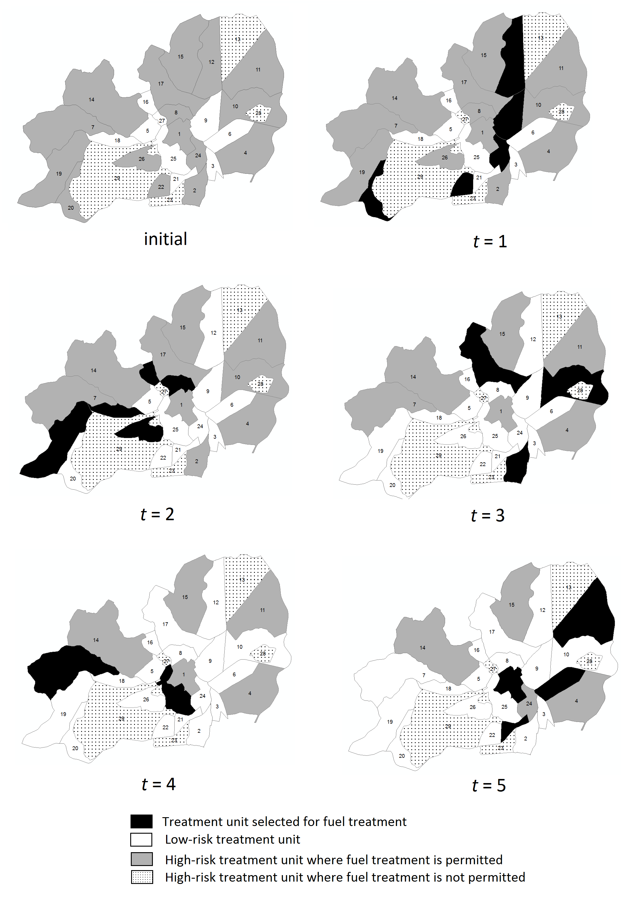
Figure 3: The sequence of maps representing the fuel treatment schedule (in years) for the test landscape

We evaluate the test landscape based on the data from Table 2. The rule is that if more than 50 percent of the treatment unit are high-risk patches, then we consider it as a high-risk treatment unit. Figure (2) and (3) show the network and the related map representing the fuel treatment schedule with 15 percent treatment level, starting from the t = 0 which represents the initial condition of the landscape. We can treat the surrounding treatment units to break the connectivity of high-risk units. When the patch within a treatment unit has reached the maximum TFI, and no patch is below the minimum TFI, the treatment units should be treated. This ecological requirement applies even for the treatment units that do not contribute to the connectivity of high-risk areas.

6 An Australian case study

Figure 4:

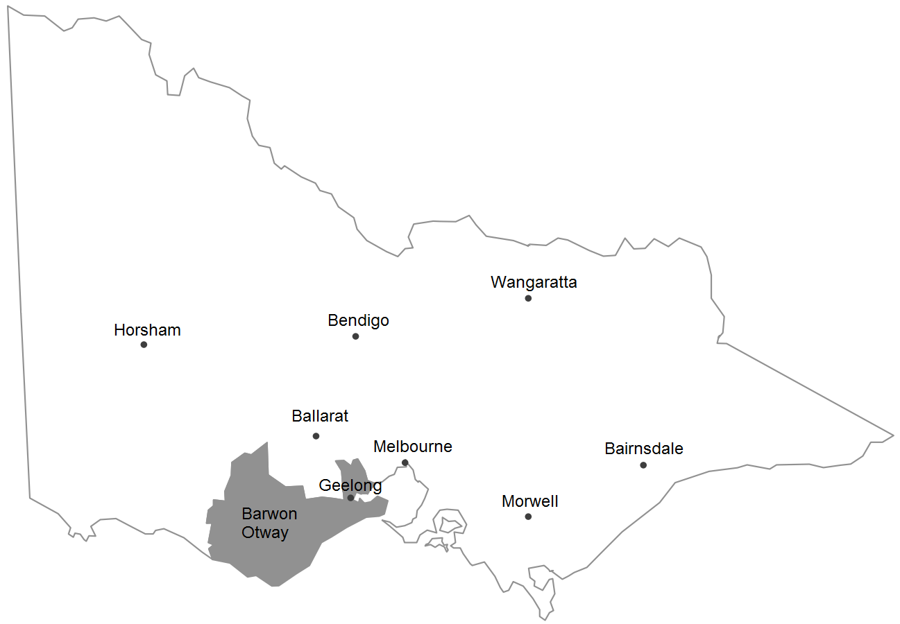
(a) Location of the case study in the Barwon-Otway district of Victoria, Australia

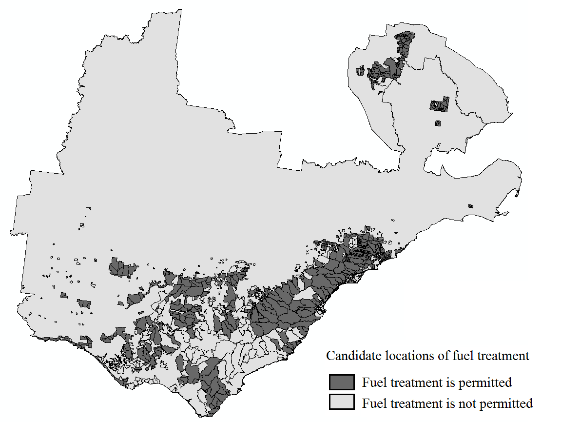
(b) Map showing the distribution of the candidate treatment units within case study area in the Barwon-Otway district of Victoria, Australia

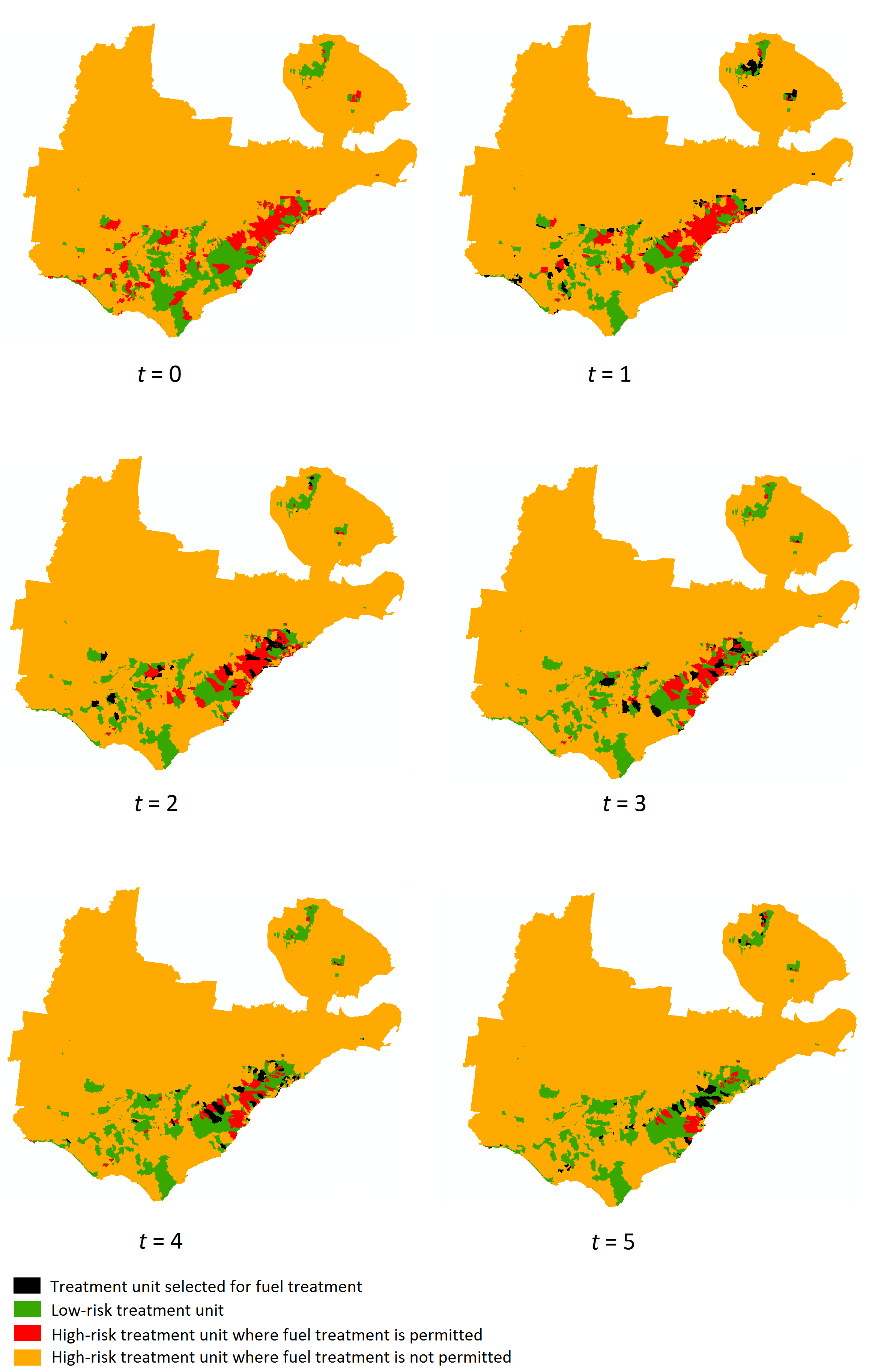
Figure 5: Solution of Phase 2: Maps showing the location of fuel treatment and the spatial distribution of high-risk treatment units over time (in years)

Table 3: Ecological Vegetation Class (EVC) and the associated threshold age, the minimum and the maximum TFI

EVC name	min TFI (year)	max TFI (year)	threshold (year)
Creekline Grassy Woodland	20	150	20
Hills Herb-rich Woodland	15	150	17
Creekline Herb-rich Woodland	15	150	17
Grassy Woodland	5	45	17
Valley Slopes Dry Forest	10	100	17
Sedgy Riparian Woodland	20	85	20
Scoria Cone Woodland	4	15	15
Wet Forest	45	300	45
Shrubby Wet Forest	25	150	25
Riparian Forest	10	80	22
Swampy Riparian Woodland	15	125	22
Riparian Scrub or Swampy Riparian Woodland Complex	10	80	16
Wet Sands Thicket	15	90	16
Stream Bank Shrubland	15	90	16
Cool Temperate Rainforest	45	999	45
Wet Heathland	12	45	12
Damp Heath Scrub	10	90	10
Damp Heath Scrub/Heathy Woodland Complex	10	90	10
Sand Heathland	8	45	8
Clay Heathland	10	45	10
Coastal Dune Scrub or Coastal Dune Grassland Mosaic	10	90	17
Coastal Headland Scrub	8	90	17
Coastal Headland Scrub/Coastal Tussock Grassland Mosaic	8	90	17
Coast Gully Thicket	10	90	17
Coastal Alkaline Scrub	10	70	17
Coastal Saltmarsh/Mangrove Shrubland Mosaic	8	90	14
Coastal Tussock Grassland	5	40	6
Heathy Woodland	5	45	35
Shrubby Woodland	10	45	35
Lowland Forest	8	80	20
Heathy Dry Forest	10	45	20
Shrubby Dry Forest	5	45	20
Grassy Dry Forest	5	45	15
Herb rich Foothill Forest	8	90	15
Shrubby Foothill Forest	8	90	15
Herb-rich Foothill Forest/Shrubby Foothill Forest Complex	8	90	15
Damp Sands Herb Rich Woodland	10	90	17
Valley Grassy Forest	10	100	17
Plains Grassy Woodland	4	15	15
Alluvial Terraces Herb-Rich Woodland	4	15	15

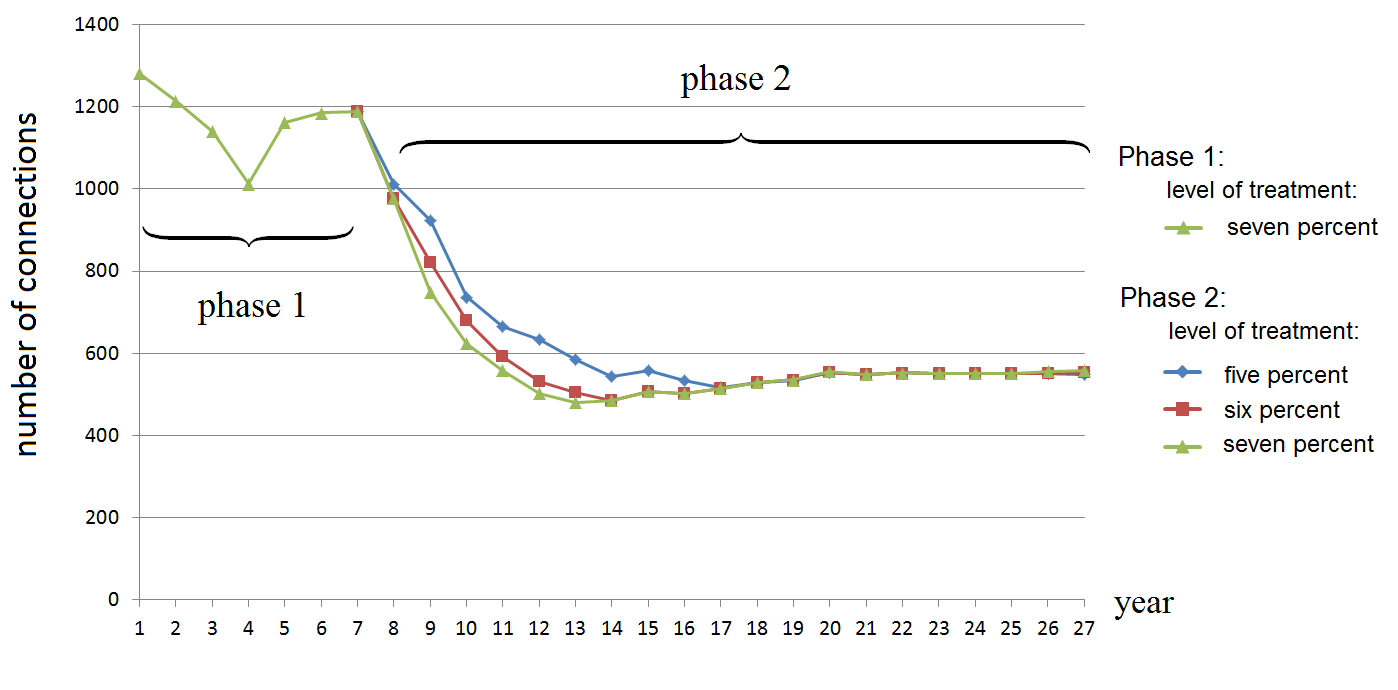
Figure 6: The number of connected high-risk treatment units over time

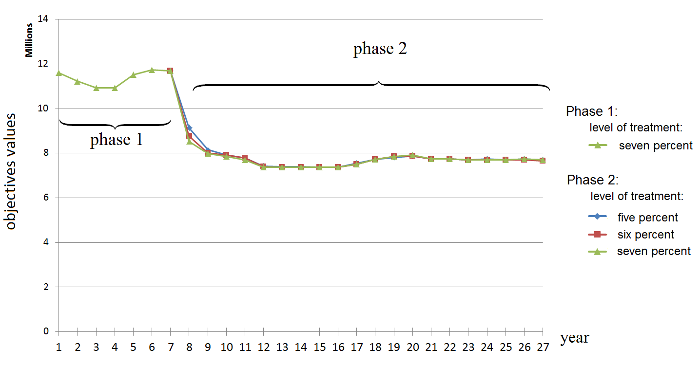
Figure 7: The objective function values over time

Table 4: Computational comparison between the five, six and seven percent treatment levels

Length of planning horizon	Solution time (seconds)
	five percent	six percent	seven percent
5 years	22.32	13.12	11.72
10 years	462.44	38.29	17.62
15 years	4904.10	752.11	366.71
20 years	26652.91	9464.17	2384.15

In this section, we apply the model discussed in Section 3 to an Australian case study. We use a real landscape with randomised data containing treatable patches, grouped into 1197 treatment units. Figure 4a illustrates the location of the case study in the Barwon-Otway district of Victoria, Australia. In this case study, we assume that we can only treat the public treatment units. Figure 4b represents the 711 candidate locations for fuel treatment. The data includes area, vegetation type and age. The minimum TFI, maximum TFI and the high-risk age threshold for each vegetation is summarised in Table 3. The vegetation types that do not pose any threat such as aquatic vegetation types are excluded in this paper. Threshold values are set to their assumed values to demonstrate our approach rather than to provide an actual way of determining these values.

A set of connected treatment units is defined as a treatment unit directly adjacent to another treatment unit, in other words, having a shared boundary. It is acknowledged it is possible for treatment units that are geographically separated to still be considered ‘connected’ as a result of the spotting behaviour of particular bark fuel types under given weather conditions. The provision of information regarding bark fuel types and prevailing weather conditions for the case study area would be a simple addition to model.

From the initial data, it was identified that 31 percent of the total treatable area in the landscape is high-risk treatable treatment units containing the patches that are over maximum TFI and no young patches. Phase 1 is run for seven percent treatment level, and would need seven years to achieve less than five percent high-risk treatment units containing old patches in the landscape. In Phase 2, we run the model presented in Section 3 for five, six and seven percent treatment levels. The solutions representing the high-risk area over time and the location selected for fuel treatments each year with seven percent treatment level can be seen in Figure 5. In this case study, we use the area of the two connected high-risk treatment unit as a weight to determine the relative importance of the connectivity. However, this weight can be determined in another way, for example, by the proportion of the shared boundary between two adjacent treatment units to the perimeter of the treatment units. It can even be adjusted subjectively by the land manager if required. Figure 6 and 7 show that the number of connectivity of high-risk treatment units in the landscape and the objective function values have the trends to decrease over time. The average of the number of connections for five, six and seven percent treatment levels are 608, 579 and 569, respectively.

The model was solved using ILOG CPLEX 12.6 with the Python 2.7 programming language using PuLP modeler. Computational experiments were performed on Trifid, a V3 Alliance high-performance computer cluster. The computational experiment used a single node with 16 cores of Intel Xeon E5-2670 64 GB of RAM. The comparison of computational time between the three different treatment levels can be seen in Table 4. For the ten-year planning horizon, the computational time for the three treatment levels is less than 15 minutes. For the longer planning horizon, the computational time becomes longer. The optimal solution can be obtained up to 20-year planning horizon.

7 Conclusion

In this paper, we have presented a mixed integer programming based approach to schedule fuel treatments. The model determines when, and where, to conduct the fuel treatment to reduce the fuel hazards in the landscape whilst still meeting ecological requirements. The ecological requirements considered in this paper are the minimum and maximum Tolerable Fire Intervals (TFI) for the vegetation present. The model includes multiple vegetation types and ages in the landscape and tracks the age of vegetation in each treatment unit. To avoid deadlocks, the rules that are applied in the model are either: the treatment unit must be treated if there is an old patch in a treatment unit, or the treatment unit cannot be treated if there is a young patch in a treatment unit. In this study, spatial and temporal changes that include multiple vegetation types in a more realistic polygon-based network representation of the landscape are considered. These improve upon previous work which was limited to a single vegetation type in a regular grid, and create a more realistic approach to fuel treatment planning for land managers.

The model was illustrated in fuel treatment planning using real landscape data from the Barwon-Otway district in south-west Victoria, Australia. We ran the model for a 20-year planning horizon with five, six and seven treatment levels. The total connectivity of high-risk regions resulting from the three different treatment levels in the landscape differs substantially for the first five years and differs slightly after five years. Based on our experiments, using seven percent treatment level, the high-risk regions in the landscape can be fragmented more quickly than that of five and six percent, as expected. From the case study, the solution of this complex multi-period model can be obtained in a reasonable computational time (eight hours). Future work is planned to extend this study by including habitat connectivity for fauna in the landscape while still fragmenting high-risk areas.

Ramya Rachmawati

Mathematics Department Faculty of Mathematics and Natural Sciences, University of Bengkulu, Bengkulu, Indonesia

School of Mathematical and Geospatial Sciences RMIT University, Melbourne, Australia

(ramya.rachmawati@rmit.edu.au)

Melih Ozlen

School of Mathematical and Geospatial Sciences RMIT University, Melbourne, Australia

(melih.ozlen@rmit.edu.au)

Karin J. Reinke

School of Mathematical and Geospatial Sciences RMIT University, Melbourne, Australia

(karin.reinke@rmit.edu.au)

John W. Hearne

School of Mathematical and Geospatial Sciences RMIT University, Melbourne, Australia

(john.hearne@rmit.edu.au)

References

- Ager et al. (2010) Ager, A., N. Vaillant, and M. Finney (2010). A comparison of landscape fuel treatment strategies to mitigate wildland fire risk in the urban interface and preserve old forest structure. Forest Ecology and Management 259(8), 1556–1570.
- Boer et al. (2009) Boer, M., R. Sadler, R. Wittkuhn, L. McCaw, and P. Grierson (2009). Long-term impacts of prescribed burning on regional extent and incidence of wildfires-evidence from 50 years of active fire management in SW Australian forests. Forest Ecology and Management 259(1), 132–142.
- Bradstock et al. (2012) Bradstock, R., G. Cary, I. Davies, D. Lindenmayer, O. Price, and R. Williams (2012). Wildfires, fuel treatment and risk mitigation in australian eucalypt forests: Insights from landscape-scale simulation. Journal of Environmental Management 105, 66–75.
- Burrows (2008) Burrows, N. (2008). Linking fire ecology and fire management in South-West Australian forest landscapes. Forest Ecology and Management 255(7), 2394 – 2406.
- Burrows and Wardell-Johnson (2003) Burrows, N. and G. Wardell-Johnson (2003). Fire and plant interactions in forested ecosystems of south-west Western Australia. Fire in ecosystems of south-west Western Australia: impacts and management 2, 225.
- Cheal (2010) Cheal, D. (2010). Growth stages and tolerable fire intervals for Victoria’s native vegetation data sets. In Fire and adaptive management report no. 84. Department of Sustainability and Environment, East Melbourne, Victoria, Australia.
- Chung (2015) Chung, W. (2015). Optimizing fuel treatments to reduce wildland fire risk. Current Forestry Reports, 1–8.
- Collins et al. (2010) Collins, B., S. Stephens, J. Moghaddas, and J. Battles (2010). Challenges and approaches in planning fuel treatments across fire-excluded forested landscapes. Journal of Forestry 108(1), 24–31.
- Ferreira et al. (2011) Ferreira, L., M. Constantino, and J. Borges (2011). A stochastic approach to optimize maritime pine (pinus pinaster ait.) stand management scheduling under fire risk. An application in Portugal. Annals of Operations Research, 1–19.
- Finney (2007) Finney, M. (2007). A computational method for optimising fuel treatment locations. International Journal of Wildland Fire 16(6), 702–711.
- Garcia-Gonzalo et al. (2011) Garcia-Gonzalo, J., T. Pukkala, and J. Borges (2011). Integrating fire risk in stand management scheduling. an application to Maritime pine stands in Portugal. Annals of Operations Research, 1–17.
- Kim et al. (2009) Kim, Y.-H., P. Bettinger, and M. Finney (2009). Spatial optimization of the pattern of fuel management activities and subsequent effects on simulated wildfires. European Journal of Operational Research 197(1), 253–265.
- King et al. (2008) King, K., R. Bradstock, G. Cary, J. Chapman, and J. Marsden-Smedley (2008). The relative importance of fine-scale fuel mosaics on reducing fire risk in South-West Tasmania, Australia. International Journal of Wildland Fire 17(3), 421–430.
- Krivtsov et al. (2009) Krivtsov, V., O. Vigy, C. Legg, T. Curt, E. Rigolot, I. Lecomte, M. Jappiot, C. Lampin-Maillet, P. Fernandes, and G. Pezzatti (2009). Fuel modelling in terrestrial ecosystems: An overview in the context of the development of an object-orientated database for wild fire analysis. Ecological Modelling 220(21), 2915–2926.
- Loehle (2004) Loehle, C. (2004). Applying landscape principles to fire hazard reduction. Forest Ecology and Management 198(1-3), 261–267.
- McCaw (2013) McCaw, L. (2013). Managing forest fuels using prescribed fire - a perspective from southern Australia. Forest Ecology and Management 294, 217–224.
- Minas et al. (2014) Minas, J., J. Hearne, and D. Martell (2014). A spatial optimisation model for multi-period landscape level fuel management to mitigate wildfire impacts. European Journal of Operational Research 232(2), 412–422.
- Penman et al. (2011) Penman, T., F. Christie, A. Andersen, R. Bradstock, G. Cary, M. Henderson, O. Price, C. Tran, G. Wardle, R. Williams, et al. (2011). Prescribed burning: how can it work to conserve the things we value? International Journal of Wildland Fire 20(6), 721–733.
- Rachmawati et al. (2015) Rachmawati, R., M. Ozlen, K. Reinke, and J. Hearne (2015). A model for solving the prescribed burn planning problem. SpringerPlus 4(1).
- Rytwinski and Crowe (2010) Rytwinski, A. and K. A. Crowe (2010). A simulation-optimization model for selecting the location of fuel-breaks to minimize expected losses from forest fires. Forest Ecology and Management 260(1), 1 – 11.
- Schmidt et al. (2008) Schmidt, D., A. Taylor, and C. Skinner (2008). The influence of fuels treatment and landscape arrangement on simulated fire behavior, Southern Cascade range, California. Forest Ecology and Management 255(8-9), 3170–3184.
- Van Wagtendonk (1995) Van Wagtendonk, J. W. (1995). Large fires in wilderness areas. United States Department of Agriculture Forest Service General Technical Report Int, 113–116.
- Wei and Long (2014) Wei, Y. and Y. Long (2014). Schedule fuel treatments to fragment high fire hazard fuel patches. Mathematical and Computational Forestry & Natural-Resource Sciences (MCFNS) 6(1), 1–10.