Work/Precision Tradeoffs in Continuum Models of Biomolecular Electrostatics

Abstract

The structure and function of biological molecules are strongly influenced by the water and dissolved ions that surround them. This aqueous solution (solvent) exerts significant electrostatic forces in response to the biomolecule’s ubiquitous atomic charges and polar chemical groups. In this work, we investigate a simple approach to numerical calculation of this model using boundary-integral equation (BIE) methods and boundary-element methods (BEM). Traditional BEM discretizes the protein–solvent boundary into a set of boundary elements, or panels, and the approximate solution is defined as a weighted combination of basis functions with compact support. The resulting BEM matrix then requires integrating singular or near singular functions, which can be slow and challenging to compute. Here we investigate the accuracy and convergence of a simpler representation, namely modeling the unknown surface charge distribution as a set of discrete point charges on the surface. We find that at low resolution, point-based BEM is more accurate than panel-based methods, due to the fact that the protein surface is sampled directly, and can be of significant value for numerous important calculations that require only moderate accuracy, such as the preliminary stages of rational drug design and protein engineering

INTRODUCTION

Protein structure and function are determined, in large part, by electrostatic interactions between the protein’s atomic charges and the surrounding biological solvent, a complex mixture of polar water molecules and dissolved charged ions [1]. Biological scientists have traditionally modeled these interactions using macroscopic continuum models based on the Debye–Hückel theory or Poisson–Boltzmann equation [1, 2]. Mean-field theories of this type assume that solvent molecules are infinitely small compared to the biomolecule solute [3], a simplification critical to the theoretical studies using spherical and ellipsoidal models of protein shapes [4]. In order to accomodate more complex molecular boundaries, the Boundary Element Method has been widely used [5, 6].

In this paper, we investigate the tradeoff between work and accuracy for representative variants of the BEM discretization, and quantify the dependence of this tradeoff on mesh resolution and the geometric complexity of the molecular boundary. Many important computations require only modest accuracy, such as the preliminary stages of rational drug design and protein engineering, and therefore could benefit from a method with a favorable ratio of flops to accuracy in this regime. We generate work-precision diagrams comparing panel and point versions of the boundary element method using the PETSc libraries.

MODEL

We will model the problem of protein solvation using the Polarizable Continuum Model (PCM) [7, 8, 9, 10]. Thus we consider a single protein in an infinite solution. In the exterior region, which we label $I$, the potential $\phi$ obeys Laplace’s equation $\nabla^{2}\phi=0$ [2], and the dielectric constant is labeled $\epsilon_{I}$, which is often taken to be 80, approximately that of bulk water. For simplicity, we omit the source term used in the linearized Poisson-Boltzmann formulation, since it will not change the arithmetic complexity of our problem. The protein interior, labeled $III$, is a low-dielectric medium, with $\epsilon_{III}$ usually between 2 and 8. It contains $Q$ discrete point charges, and the potential satisfies a Poisson equation $\nabla^{2}\phi=\sum^{Q}_{k}q_{k}\delta(\vec{r}-\vec{r}_{k})$ where $q_{k}$ and $\vec{r}_{k}$ specify the $k$th charge. The boundary $a$ separates the protein region $III$ from the solvent $I$. The potential is assumed to decay to zero suitably fast as $\vec{r}\to\infty$, and the boundary conditions are continuity of the potential and displacement field,

$$\phi_{I}(\vec{r}_{a}) =\phi_{III}(\vec{r}_{a}),$$ (1)

$$\epsilon_{I}\frac{\partial\phi_{I}(\vec{r}_{a})}{\partial n} =\epsilon_{III}\frac{\partial\phi_{III}(\vec{r}_{a})}{\partial n}.$$ (2)

If we insert the free space Green’s function for the potential into the second boundary condition, we obtain a Boundary Integral Equation [11, 12] for the induced surface charge on $a$,

$$\sigma(\vec{r})+\hat{\epsilon}\int_{a}\frac{\partial}{\partial n(\vec{r})}\frac{\sigma(\vec{r}^{\prime})d^{2}\vec{r}^{\prime}}{4\pi|\vec{r}-\vec{r}^{\prime}|}=-\hat{\epsilon}\sum^{Q}_{k=1}\frac{\partial}{\partial n(\vec{r})}\frac{q_{k}}{4\pi|\vec{r}-\vec{r}_{k}|}.$$ (3)

We can write this more compactly using the adjoint of the double layer operator $K$ and the operator $B$ which gives the normal electric field due to a unit charge,

$$\left(I+\hat{\epsilon}K^{*}\right)\sigma =B\vec{q}$$ (4)

$$A\sigma =B\vec{q}$$ (5)

where $\vec{q}$ is the vector of charge values and we introduce an operator $A$.

The solvation free energy is the energy of interaction between the induced surface charge, or solvent polarization, and the solute charges. In order to calculate solvation energies, we will first find the reaction potential $\psi$, which is the potential due to the induced surface charge $\sigma$. We define an operator $C$ which gives this mapping,

$$\psi(\vec{r})=C\sigma(\vec{r})=\int_{a}\frac{\sigma(\vec{r}^{\prime})d^{2}\vec{r}^{\prime}}{4\pi\epsilon_{I}|\vec{r}-\vec{r}^{\prime}|}.$$ (6)

Now we can write the full expression for the solvation energy $E$ in the simple form

$$E=\vec{q}^{T}CA^{-1}B\vec{q}=\vec{q}^{T}L\vec{q},$$ (7)

where we introduce the reaction potential matrix $L$ which has dimensions $Q\times Q$. We will be interested in the approximation of $L$ below, since it determines the quantity of interest for our biological problems.

PANEL DISCRETIZATION

A common approach to the discretization of Eq. 3 is the Galerkin method [13, 14], in which the residual is not required to vanish pointwise, but rather to be orthogonal to a set of test vectors. In the limit that the test vectors form a basis for the entire approximation space, we recover the same solution as the original equation. Thus we introduce test functions $\tau_{i}(\vec{r})$, and integrate our equation

$$\int_{a}d^{2}\vec{r}\,\tau_{i}(\vec{r})\left(I+\hat{\epsilon}K^{*}\right)\sigma(\vec{r}) =$$ (8)

$$\quad\int_{a}d^{2}\vec{r}\,\tau_{i}(\vec{r})B\vec{q}$$

$$\int_{a}d^{2}\vec{r}\,\tau_{i}(\vec{r})\left(\sigma(\vec{r})+\hat{\epsilon}\int_{a}\frac{\partial}{\partial n(\vec{r})}\frac{\sigma(\vec{r}^{\prime})d^{2}\vec{r}^{\prime}}{4\pi|\vec{r}-\vec{r}^{\prime}|}\right) =$$ (9)

$$\quad-\int_{a}d^{2}\vec{r}\,\tau_{i}(\vec{r})\hat{\epsilon}\sum^{Q}_{k=1}\frac{\partial}{\partial n(\vec{r})}\frac{q_{k}}{4\pi|\vec{r}-\vec{r}_{k}|}.$$

We must decide how to discretize the integrals appearing in Eq. 8, using some sort of quadrature. Below we employ triangular panels and constant basis functions in each panel. For quadrature, we choose the qualocation strategy [15, 16], which uses a single point centroid quadrature for the inner integration over $\vec{r}^{\prime}$, and either a high-order quadrature or analytic result for the outer integration over $\vec{r}$,

$$\sum_{m}w_{m}\tau_{i}(\vec{r}_{m})\left(\sigma(\vec{r}_{m})+\hat{\epsilon}\frac{\partial}{\partial n(\vec{r}_{m})}\frac{\sigma(\vec{r}_{j})a_{j}}{4\pi|\vec{r}_{m}-\vec{r}_{j}|}\right) =$$ (10)

$$\quad-\sum_{m}w_{m}\tau_{i}(\vec{r}_{m})\hat{\epsilon}\sum^{Q}_{k=1}\frac{\partial}{\partial n(\vec{r}_{m})}\frac{q_{k}}{4\pi|\vec{r}_{m}-\vec{r}_{k}|}.$$

In the results section, we use analytic integrals, either the Hess-Smith method, or the Newman method when vector to the evaluation point is too close to the panel normal [17, 18].

In order to compute one entry in our matrices $A$ or $B$, we need to integrate over a panel and perform an evaluation at our source point. In the following, we will only consider the cost of evaluating $A$ since $B$ and $C$ are much less expensive due to the fact the $Q<<N_{c}$, where $N_{c}$ is the number of panels on the surface. Once we have our matrices $A$, $B$, and $C$, the cost to compute the $L$ matrix is dominated by the inversion of $A$, which executes $\mathcal{O}(N_{c}^{3})$ flops. If we let the relative cost of panel integration against point evaluation be $N_{p}$, then the dominant terms in our complexity model are

$$\mathcal{O}(N_{p}N_{c}^{2})+\mathcal{O}(N_{c}^{3}).$$ (11)

Clearly, as the size of the mesh grows, the time will be completely dominated by the second term. However, this is usually alleviated by using an iterative method for the inversion, which can reduce the cost to

$$\mathcal{O}(N_{p}N_{c}^{2})+\mathcal{O}(N_{c}^{2})$$ (12)

since the number of iterates is bounded by a constant independent of the size of the system because the condition number of $A$ is bounded [13]. It is also true that the exponent of $N_{c}$ can be reduced from 2 to 1 using methods that exploit the decay in the interaction with distance, such as the Fast Multipole Method [19], modified FFT methods [20], or skeletonization [21]. This will not be our main concern, since we are evaluating cost $N_{p}$ incurred by panel integration against the extra accuracy gained.

POINT DISCRETIZATION

As a lower-cost alternative to the panel discretization, we consider a collocation method which enforces the continuum equation at a given set of points $\{\vec{r}_{i}\}$, and discretize the integral operator using the Nyström method (quadrature),

$$\left(I+\hat{\epsilon}K^{*}\right)\sigma(\vec{r}_{i}) =B\vec{q}$$ (13)

$$\sigma(\vec{r}_{i})+\hat{\epsilon}\int_{a}\frac{\partial}{\partial n(\vec{r}_{i})}\frac{\sigma(\vec{r}^{\prime})d^{2}\vec{r}^{\prime}}{4\pi|\vec{r}_{i}-\vec{r}^{\prime}|} =-\hat{\epsilon}\sum^{Q}_{k=1}\frac{\partial}{\partial n(\vec{r}_{i})}\frac{q_{k}}{4\pi|\vec{r}_{i}-\vec{r}_{k}|}$$ (14)

$$\sigma(\vec{r}_{i})+\hat{\epsilon}\sum_{j}\frac{\partial}{\partial n(\vec{r}_{i})}\frac{\sigma(\vec{r}_{j})w_{j}}{4\pi|\vec{r}_{i}-\vec{r}_{j}|} =-\hat{\epsilon}\sum^{Q}_{k=1}\frac{\partial}{\partial n(\vec{r}_{i})}\frac{q_{k}}{4\pi|\vec{r}_{i}-\vec{r}_{k}|}$$ (15)

and the contribution from the $i=j$ term is 0. A similar collocation method is used to evaluate the $C$ operator. For this study, we have chosen to use the vertices of panel triangulations as the points, and the point weights are determined by giving each vertex 1/3 of the panel area for each panel incident to it.

The construction of $A$, $B$, $C$ and $L$ for the point discretization has a complexity model very similar to Eq. 12,

$$\mathcal{O}(N_{c}^{2})+\mathcal{O}(N_{c}^{2}).$$ (16)

RESULTS

We demonstrate the correctness of our implementation using a simple problem with known exact solution. Then we show that our point BEM variants can be more efficient in a certain accuracy range, using realistic test cases for amino acid residues. For all test cases, we take the dielectric constant of the solvent $\epsilon_{I}=80$, and the dielectric constant of the solute $\epsilon_{III}=4$. Initial MATLAB implementations of the panel BEM method and point BEM method are available in online repositories, along with a higher-performance implementation using the PETSc libraries [22, 23] was used to run all the tests below, and is available online [24]. All timings are from an Apple Airbook with a 1.4 GHz Core i5 processor and 8GB of 1600 MHZ DDR3 RAM.

SPHERE

As an initial test, we compare the error in the methods described above for the problem of a low-dielectric sphere in a high-dielectric medium, which has a classical exact solution [4, 12]. Specifically, we take a sphere of radius $R$ with dielectric constant $\epsilon_{III}$, embedded in a medium of dielectric constant $\epsilon_{I}$, and fill it with random charges. The charges are randomly selected from vertices on a grid of spacing $h$, where selected vertices must be at least distance $h$ from the spherical surface.

The reaction potential $\psi$, which we evaluate at each charge location $x_{j}$, is given by

$$\psi=\sum^{\infty}_{n=0}\sum^{n}_{m=-n}B_{nm}r^{n}_{j}P_{n}^{m}(\cos\theta_{j})e^{im\phi_{j}}.$$ (17)

where the reaction potential expansion coefficients are given by

$$B_{nm}=\frac{1}{\epsilon_{1}b^{2n+1}}\frac{(\epsilon_{1}-\epsilon_{2})(n+1)}{\epsilon_{1}n+\epsilon_{2}(n+1)}E_{nm},$$ (18)

and the charge distribution expansion coefficients are

$$E_{nm}=\sum^{Q}_{k=1}q_{k}r^{n}_{k}\frac{(n-|m|)!}{(n+|m|)!}P_{n}^{m}(\cos\theta_{k})e^{-im\phi_{k}}.$$ (19)

In order to demonstrate correctness, we show convergence of our solution to the analytic reference solution as the element size is reduced, and call this mesh convergence. In Fig. 1, we demonstrate mesh convergence of both BEM variants for the sphere problem. As we expect, the panel method converges with order 1, and the point method with order 1/2 [13].

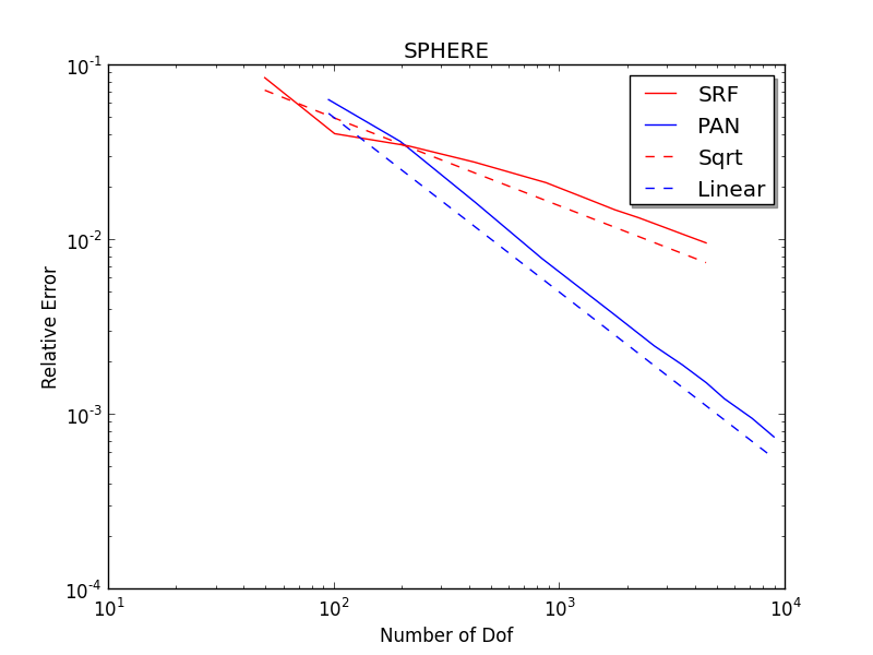
Fig. 1: WE SHOW MESH CONVERGENCE FOR BEM METHODS APPLIED TO THE PROBLEM OF RANDOM CHARGES IN A SPHERE, WITH $R=6.0$, $h=1.0$, $\epsilon_{I}=80$, $\epsilon_{III}=4$, AND $Q=10$ CHARGES. THE ANALYTIC SOLUTION IS CALCULATED TO MULTIPOLE ORDER 25. CLEARLY, THE PANEL METHOD (PAN) CONVERGES LINEARLY, AND THE POINT METHOD SRF HAS ORDER 1/2.

To show a practical case, we note that although accurate representation of the boundary is important globally, protein charges are at atom centers and therefore usually more than about 1 Angstrom from the boundary. Fig. 2 shows the potentials for single charges in the 6-Angstrom sphere: for the main plot, the charge is at $(0,0,4.5~{}\mathrm{\AA})$ and $(0,0,5.5~{}\mathrm{\AA})$ for the inset. We plot potentials along the $Z$ axis. For the $Z=4.5$ charge, the accuracy is acceptable throughout (less than 1 kcal/mol/$e$), except between the charge and the boundary. On the other hand, the error is large for the less realistic case (note that the scales are different).

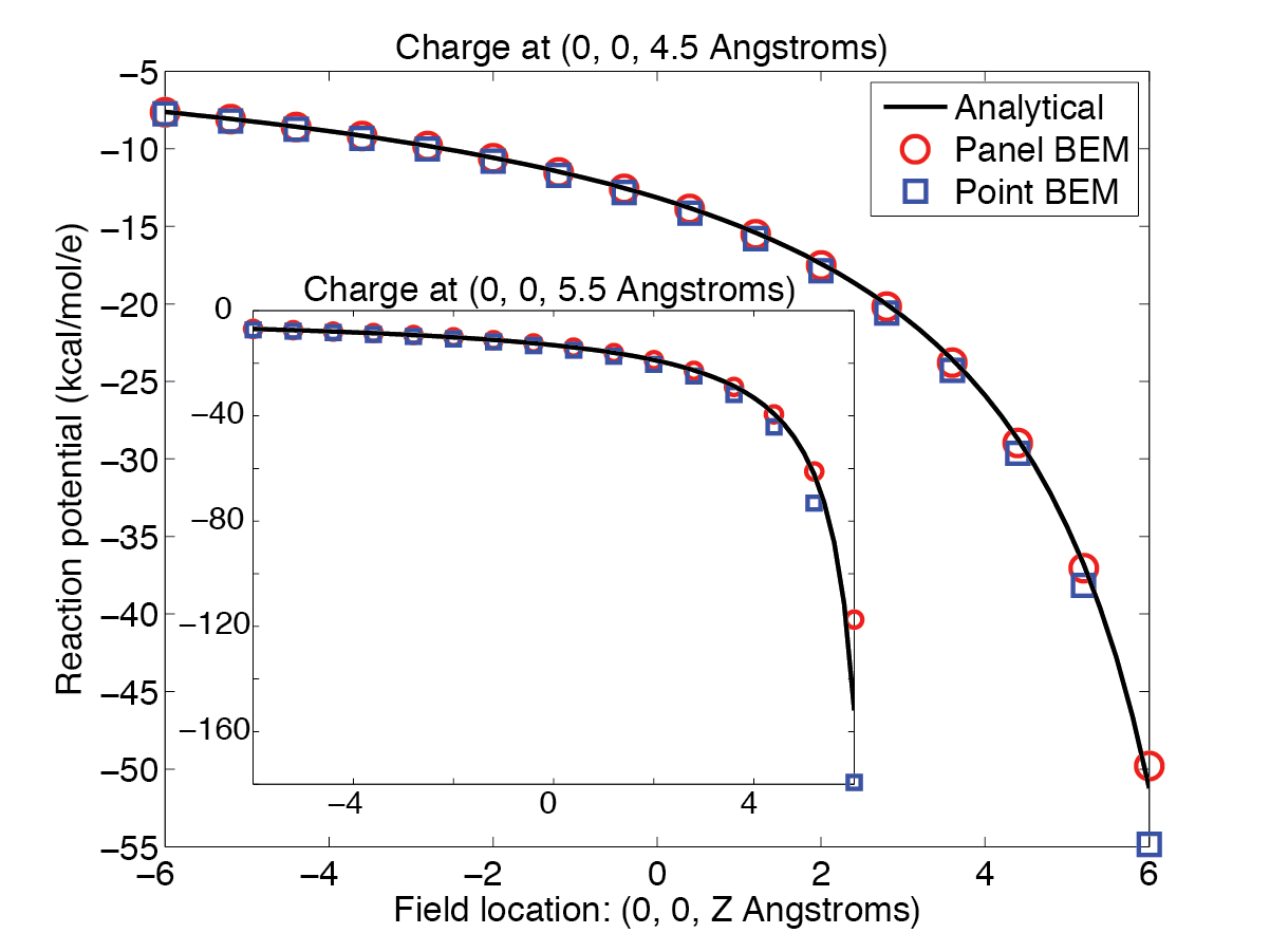
Fig. 2: WE SHOW THE RESULTING POTENTIALS FOR SINGLE CHARGES IN A SPHERE, WITH $R=6.0$, $h=1.0$, $\epsilon_{I}=80$, $\epsilon_{III}=4$. THE CHARGE IS AT (0, 0, 4.5 ANGSTROMS) FOR THE MAIN PLOT AND AT (0, 0, 5.5 ANGSTROM) FOR THE INSET. POINT BEM ACCURACY IS ACCEPTABLE FOR THE CHARGE AT 4.5 ANGSTROMS BUT NOT FOR THE ONE AT 5.5 ANGSTROMS.

In order to look more closely at the computation itself, we will employ a work-precision diagram [25]. This plots the work done against the accuracy that was achieved by the computation. We define the work as the number of floating point operations (flops) used to compute a) the reaction potential matrix $L$, and b) just the entries of $A$. We expect the second metric to map well to the case where scalable, or fast, algorithms are used for construction since the local work done for those algorithms is typically greater than half of the total, and uses exactly these routines, whereas the large number of flops in the direct inversion of $A$ dominates the total for the simpler dense case. When we examine Fig. 3, we see that to obtain errors less than 3 kcal/mol it is more advantageous to use the panel method. If we only consider the formation of the surface-to-surface operator $A$, this accuracy threshold decreases to 1.5 kcal/mol.

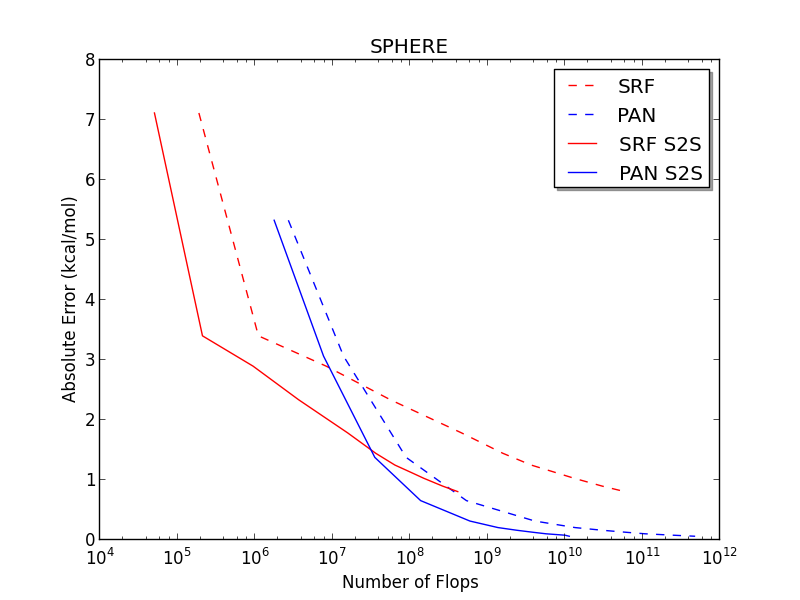
Fig. 3: WE SHOW A WORK-PRECISION DIAGRAM FOR BEM METHODS APPLIED TO THE SAME PROBLEM AS FIG. 1. FOR THIS CASE, THE PANEL METHOD IS SUPERIOR FOR ERROR BELOW 3 KCAL/MOL, ALTHOUGH WHEN ONLY CONSIDERING THE SURFACE-TO-SURFACE (S2S) OPERATOR $A$, THE POINT METHOD IS SUPERIOR DOWN TO 1.5 KCAL/MOL.

RESIDUES

To compare the discretizations on realistic, atomically detailed molecular geometries, we next look at the reaction field of two $\alpha$-amino acids, aspartic acid (ASP) and arginine (ARG). Amino acids are the building blocks of proteins, and because these and other charged amino acids play key roles in biomolecular electrostatics, accurate calculations are essential. Meshes were created for the isolated amino acid structures using the meshmaker program from the FFTSVD package [26], the MSMS program [27], PDB files from the Protein Data Bank [28], and atomic radii parameterized for the CHARMM force field [29, 30]. Using these tools, we can create a range of panel/point densities.

In Fig. 4, we show mesh convergence for ASP. It is initially noisy, but we clearly see the asymptotic convergence rates for larger meshes. We have defined the reference energy to be the result of Richardson extrapolation [31] using the last two energies from the panel method. Thus, in all residue figures the last panel method energy appears unrealistically accurate. The absolute solvation energies are shown in Fig. 5, and it is clear that the order 1/2 convergence of the point method looks like complete stagnation on the scale of our tests. The same convergence behavior is seen in Fig. 6 for ARG.

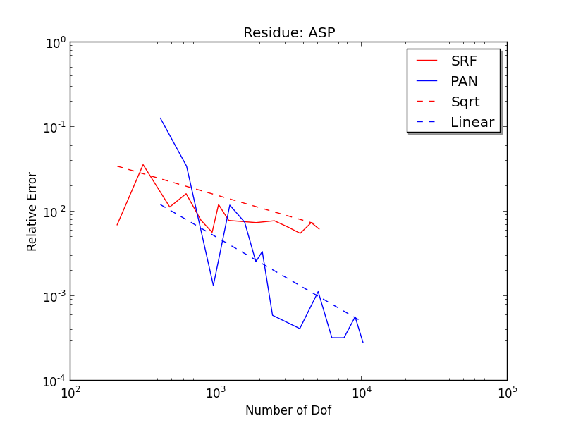
Fig. 4: WE SHOW MESH CONVERGENCE FOR BEM METHODS APPLIED TO THE ASPARTIC ACID MOLECULE, WITH $\epsilon_{I}=80$ AND $\epsilon_{III}=4$. WE AGAIN SEE THAT THE PANEL METHOD (PAN) CONVERGES LINEARLY, AND THE POINT METHOD (SRF) HAS ORDER 1/2, ALTHOUGH THE CONVERGENCE IS INITIALLY NOISY.

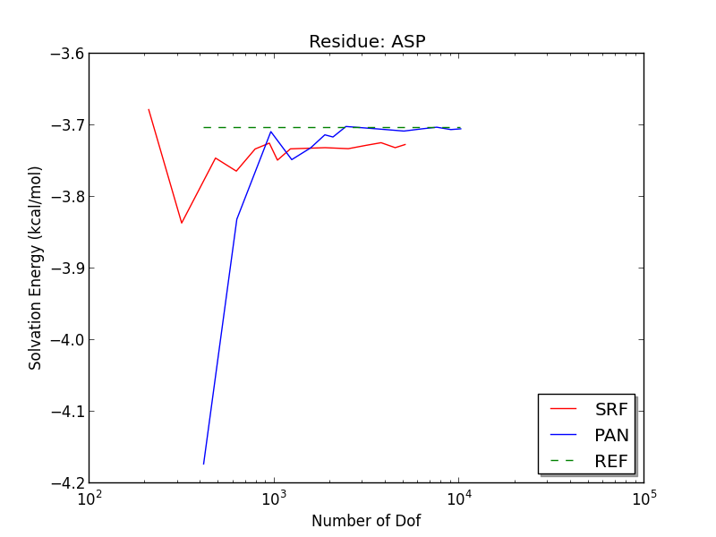
Fig. 5: WE SHOW SOLVATION ENERGY CONVERGENCE FOR BEM METHODS APPLIED TO THE ASPARTIC ACID MOLECULE ($\epsilon_{I}=80$ and $\epsilon_{III}=4$). NOTE THAT INITIALLY THE POINT METHOD CONVERGES FASTER, BUT STAGNATES SOON AFTER.

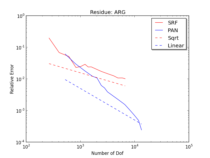
Fig. 6: WE SHOW MESH CONVERGENCE FOR BEM METHODS APPLIED TO THE ARGININE MOLECULE ($\epsilon_{I}=80$ AND $\epsilon_{III}=4$). AGAIN THE PANEL METHOD (PAN) CONVERGES LINEARLY, AND THE POINT METHOD (SRF) HAS ORDER 1/2, ALTHOUGH CONVERGENCE IS INITIALLY NOISY.

From the work-precision diagrams in Fig. 7 and Fig. 8, we see that the accuracy threshold for the point method to be preferred has moved considerably lower. In fact, when comparing construction of the surface-to-surface operator $A$, we see that the point method has lower costs up to errors of 0.25 kcal/mol, well within the range of many biological studies.

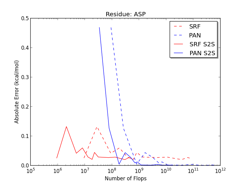
Fig. 7: WE SHOW A WORK-PRECISION DIAGRAM FOR BEM METHODS APPLIED TO THE SAME PROBLEM AS FIG. 4. FOR THIS CASE, THE PANEL METHOD IS SUPERIOR FOR ERROR BELOW 0.25 KCAL/MOL.

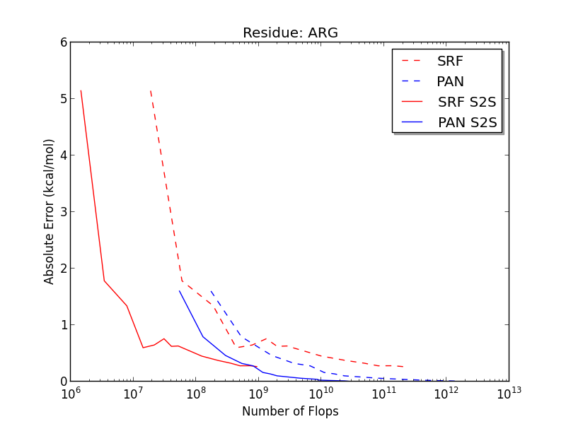
Fig. 8: WE SHOW A WORK-PRECISION DIAGRAM FOR BEM METHODS APPLIED TO THE SAME PROBLEM AS FIG. 6. FOR THIS CASE, THE PANEL METHOD IS SUPERIOR FOR ERROR BELOW 0.75 KCAL/MOL, ALTHOUGH WHEN ONLY CONSIDERING THE SURFACE-TO-SURFACE (S2S) OPERATOR $A$, THE POINT METHOD IS SUPERIOR DOWN TO 0.25 KCAL/MOL.

DISCUSSION

We have compared the work-accuracy tradeoff in panel and point BEM methods. Very clear accuracy thresholds emerge below which point BEM is preferable to the panel method. Point BEM can be used productively for scenarios that tolerate low resolution, such as intermediate calculations in design iterations, structure optimization, and optimization of binding affinity. The range of applicable problems could be expanded by optimizing the placement and weighting of points. Sophisticated tools, such as MSP [32], could be used to improve our point discretizations, and is the subject of future research.

How does our outlook change with the introduction of fast methods for the application of the integral operators? The characteristics of the local work remain identical. On modern architectures, an optimal workload roughly balances long range, or tree work, with local direct calculations [33]. Thus, the speedup we show above of point methods over panel methods should remain roughly intact. We plan to validate this claim using the PyGBe fast solver [34].

References

- [1] K. A. Sharp and B. Honig. Electrostatic interactions in macromolecules: Theory and applications. Ann. Rev. Biophys. Biophys. Chem., 19:301–332, 1990.
- [2] J. P. Bardhan. Biomolecular electrostatics—I want your solvation (model). Computational Science and Discovery, 5:013001, 2012.
- [3] D. Beglov and B. Roux. An integral equation to describe the solvation of polar molecules in liquid water. J. Phys. Chem. B, 101:7821–7826, 1997.
- [4] J. G. Kirkwood. Theory of solutions of molecules containing widely separated charges with special application to zwitterions. J. Chem. Phys., 2:351, 1934.
- [5] F. J. Rizzo. An integral equation approach to boundary value problems of classical electrostatics. Quarterly of Applied Mathematics, 25:83–95, 1967.
- [6] S. Mukherjee. Boundary element methods in solid mechanics - a tribute to Frank Rizzo. Electronic Journal of Boundary Elements, 1:47–55, 2003.
- [7] S. Miertus, E. Scrocco, and J. Tomasi. Electrostatic interactions of a solute with a continuum – a direct utilization of ab initio molecular potentials for the prevision of solvent effects. Chem. Phys., 55(1):117–129, 1981.
- [8] R. Cammi and J. Tomasi. Remarks on the apparent-surface charges (ASC) methods in solvation problems: Iterative versus matrix-inversion procedures and the renormalization of the apparent charges. J. Comput. Chem., 16(12):1449–1458, 1995.
- [9] E. Cancès, B. Mennucci, and J. Tomasi. A new integral equation formalism for the polarizable continuum model: Theoretical background and applications to isotropic and anisotropic dielectrics. J. Chem. Phys., 107(8):3032–3041, 1997.
- [10] B. Mennucci. Continuum solvation models: what else can we learn from them? J. Phys. Chem. Lett., 1:1666–1674, 2010.
- [11] M. D. Altman, J. P. Bardhan, J. K. White, and B. Tidor. Accurate solution of multi-region continuum electrostatic problems using the linearized Poisson–Boltzmann equation and curved boundary elements. J. Comput. Chem., 30:132–153, 2009.
- [12] J. P. Bardhan and M. G. Knepley. Mathematical analysis of the boundary-integral based electrostatics estimation approximation for molecular solvation: Exact results for spherical inclusions. J. Chem. Phys., 135:124107, 2011.
- [13] K. E. Atkinson. The Numerical Solution of Integral Equations of the Second Kind. Cambridge University Press, 1997.
- [14] C. Pozrikidis. A Practical Guide to Boundary-Element Methods with the Software Library BEMLIB. Chapman & Hall/CRC Press, 2002.
- [15] J. Tausch, J. Wang, and J. White. Improved integral formulations for fast 3-D method-of-moment solvers. IEEE T. Comput.-Aid. D., 20(12):1398–1405, 2001.
- [16] J. P. Bardhan. Numerical solution of boundary-integral equations for molecular electrostatics. J. Chem. Phys., 130:094102, 2009.
- [17] J. L. Hess and A. M. O. Smith. Calculation of non-lifting potential flow about arbitrary three-dimensional bodies. J. Ship Res., 8(2):22–44, 1962.
- [18] J. N. Newman. Distribution of sources and normal dipoles over a quadrilateral panel. J. Eng. Math., 20(2):113–126, 1986.
- [19] L. Greengard. The Rapid Evaluation of Potential Fields in Particle Systems. MIT Press, 1988.
- [20] M. D. Altman, J. P. Bardhan, B. Tidor, and J. K. White. FFTSVD: A fast multiscale boundary-element method solver suitable for bio-MEMS and biomolecule simulation. IEEE T. Comput. Aid. D., 25:274–284, 2006.
- [21] K. L. Ho and L. Greengard. A fast direct solver for structured linear systems by recursive skeletonization. SIAM Journal of Scientific Computing, 34:A2507–A2532, 2012.
- [22] Satish Balay, Jed Brown, Kris Buschelman, William D. Gropp, Dinesh Kaushik, Matthew G. Knepley, Lois Curfman McInnes, Barry F. Smith, and Hong Zhang. PETSc Web page, 2011. http://www.mcs.anl.gov/petsc.
- [23] Satish Balay, Jed Brown, , Kris Buschelman, Victor Eijkhout, William D. Gropp, Dinesh Kaushik, Matthew G. Knepley, Lois Curfman McInnes, Barry F. Smith, and Hong Zhang. PETSc users manual. Technical Report ANL-95/11 - Revision 3.2, Argonne National Laboratory, 2011.
- [24] Matthew Knepley and Jaydeep P. Bardhan. PETSc Point BEM. https://bitbucket.org/knepley/pointbem-petsc, 2015.
- [25] Ernst Hairer, Syvert P Nørsett, and Gerhard Wanner. Solving ordinary differential equations i: Nonstiff problems. 2009.
- [26] M. D. Altman, J. P. Bardhan, B. Tidor, and J. K. White. FFTSVD: A fast multiscale boundary-element method solver suitable for BioMEMS and biomolecule simulation. IEEE T. Comput.-Aid. D., 25:274–284, 2006.
- [27] M. Sanner, A. J. Olson, and J. C. Spehner. Reduced surface: An efficient way to compute molecular surfaces. Biopolymers, 38:305–320, 1996.
- [28] H. M. Berman, J. Westbrook, Z. Feng, G. Gilliland, T. N. Bhat, H. Weissig, I. N. Shindyalov, and P. E. Bourne. The protein data bank. Nucleic Acids Res., 28(1):235–242, 2000.
- [29] B. R. Brooks, R. E. Bruccoleri, B. D. Olafson, D. J. States, S. Swaminathan, and M. Karplus. CHARMM: A program for macromolecular energy, minimization, and dynamics calculations. J. Comput. Chem., 4:187–217, 1983.
- [30] M. Nina, D. Beglov, and B. Roux. Atomic radii for continuum electrostatics calculations based on molecular dynamics free energy simulations. J. Phys. Chem. B, 101:5239–5248, 1997.
- [31] Lewis Fry Richardson. The approximate arithmetical solution by finite differences of physical problems including differential equations, with an application to the stresses in a masonry dam. Philosophical Transactions of the Royal Society A, 210(459–470):307–357, 1911.
- [32] Michael L. Connolly. Molecular surface package (MSP). http://biohedron.drupalgardens.com/, 2015.
- [33] L. Greengard and W. D. Gropp. A parallel version of the fast multipole method. Comp. Math. Appl., 20(7):63–71, 1990.
- [34] C. D. Cooper, J. P. Bardhan, and L. A. Barba. A biomolecular electrostatics solver using Python, GPUs and boundary elements that can handle solvent-filled cavities and Stern layers. Comput. Phys. Commun., 185:720–729, 2013.