Inferring Volatility in the Heston Model and its Relatives – an Information Theoretical Approach

Abstract

Stochastic volatility models describe asset prices $S_{t}$ as driven by an unobserved process capturing the random dynamics of volatility $\sigma_{t}$. Here, we quantify how much information about $\sigma_{t}$ can be inferred from asset prices $S_{t}$ in terms of Shannon’s mutual information $I(S_{t}:\sigma_{t})$.

This motivates a careful numerical and analytical study of information theoretic properties of the Heston model. In addition, we study a general class of discrete time models motivated from a machine learning perspective. In all cases, we find a large uncertainty in volatility estimates for quite fundamental information theoretic reasons.

Index terms— Information Theory; Stochastic Volatility; Bayesian Analysis

1 Introduction

Many plaudits have been aptly used to describe Black and Scholes’ [4] contribution to option pricing theory. However, especially after the 1987 crash, the geometric Brownian motion model and the Black-Scholes formula were unable to reproduce the option price data of real markets. This is not surprising, since the Black-Scholes model makes the strong assumption that log-returns of stocks are normally distributed with a volatility which is not only assumed to be known but also constant over time. Both assumptions on volatility are wrong: first, volatility is a hidden parameter which needs to be inferred from stock and option data, respectively; second, this so called “implied volatility” is not constant at all but a highly volatile time-process. The second insight led to the introduction of implied volatility indices like the VIX (1993) and its off-springs, based on the work [8, 9], which make implied volatility a trademark in its own right subject to similar stochastic movements as stock prices. Among the most relevant statistical properties of these implied volatility processes, volatility seems to be responsible for the observed clustering in price changes. That is, large fluctuations are commonly followed by other large fluctuations and similarly for small changes [7]. Another feature is that, in clear contrast with price changes which show negligible autocorrelations, volatility autocorrelation is still significant for time lags longer than one year [35, 32, 7, 28, 14, 27]. Additionally, there exists the so-called leverage effect, i.e., much shorter (few weeks) negative cross-correlation between current price change and future volatility [6, 7, 4, 5].
Accompanying these empirical findings on volatility processes there is also a long history of theoretical attempts to map the time dependency of volatility via stochastic processes – see [40] for an extensive review of the literature. The first stochastic volatility model directly addressing the observed effect of volatility clustering is the one of Taylor [42] – a univariate time-discrete autoregression. [33] investigate those ARCH models and their generalized descendants, GARCH and EGARCH, how they estimate conditional variances and covariances properly even in the case they are misspecified.
Continuous time models were introduced by Johnson [24]. The best known paper in this area is Hull and White [22]. Heston’s model [21], giving rise to a gamma distributed volatility, is very popular, thanks to the fact that it has a closed-form expression for the characteristic function of its transitional probability. Research in the late 1990s and early 2000s has shown that more complicated stochastic volatility models are needed to model either option or high frequency data since the previously mentioned models do not deal properly with significant changes of volatility on a short time scale. Thus, jumps were incorporated in stochastic volatility [16, 17] and in [12] affine jump-diffusion processes are treated analytically deriving closed form solutions for call options as Heston obtained for his model [21]. There are also approaches which model the volatility process as a function of a number of separate stochastic processes or factors. In [10] two-factor models are studied with one very slowly mean reverberating factor and another quickly mean reverting one. Such two-factor models provide an alternative to jump-diffusions in breaking the link between tail thickness and volatility persistence. [31] investigates an exponential Ornstein-Uhlenbeck stochastic volatility model and observes that the model shows a multi-scale behaviour in the volatility autocorrelation. It also exhibits a leverage correlation and a probability profile for the stationary volatility which are consistent with market observations. All these features make the model quite appealing since it appears to be more complete than other stochastic volatility models also based on a two-dimensional diffusion discussed in [10]. In summary, there is a vast literature on stochastic volatility models investigating and discussing to which extend those models fit with the data and reproduce the statistical properties of realised volatility of stocks: temporal clustering, leverage effect, volatility autocorrelation, empirical option prices, and the temporal evolution of volatility. Furthermore, papers like [10] and [33] strive identify the best model on empirical grounds. I.e., these papers use statistical tests to decide which stochastic volatility models do best in fitting real world data, such as stock prices, volatility indices, etc. Hence, the entire literature reviewed in [40] tackles mainly the second previously listed issue with volatility in the classical Black-Scholes model: its time dependency.
The approach presented in this paper has a different focus: Assuming that a stochastic volatility model is correct, i.e., stock prices and daily returns, respectively, follow its dynamics, how reliably can the hidden volatility inferred from those data according to the stochastic volatility model describing this data precisely. That is, compared to the previously cited papers, we particularly stress the problem arising from the first mentioned problem concerning Black and Scholes model: the hidden nature of volatility and the only possibility to grasp it via implied volatility derived from market data. If stochastic volatility models describe financial markets properly, how reliable is implied volatility as a volatility measurement. That is, how much information about volatility can be derived from stock data as its observable? Since stochastic volatility models deal with two different distributions for the stock process $S_{t}$ and its volatility process $\sigma_{t}$, Shannon’s information theory [39] provides an ideal frame to make this question precise: What is the mutual information $I(S_{t}:\sigma_{t})$ between the observed stock prices $S_{t}$ and the hidden volatility process $\sigma_{t}$? Among the vast amount of stochastic volatility models choices have to be made. First, we consider Heston’s model [21] because the closed form solution of the transitional probabilities of the joint stock and volatility process is analytically appealling. Second, the purely theoretical studies on the Heston model are accompanied by an empirical survey on exponential Ornstein-Uhlenbeck single- and two-factor model which are suggested by [31] as stochastic volatility models fitting observed data best. Hence, the models have been chosen with respect to their claimed theoretical and empirical advantages, respectively, even though we believe the results obtained in the present paper to prevail among a wide class of models.

These results are quite disillusioning. Via numerical computations we were able to compute the evolution of the mutual information $I(\sigma_{t}:S_{t})$ over time in the Heston model for parameters derived from the VIX in [2]. It is at most about $0.5$ bit and seems even to diminish for $t\rightarrow\infty$. A further interesting finding is the existence of a local maximum of the function $t\rightarrow I(\sigma_{t}:S_{t})$ suggesting that there is an intermediate time scale at which the two processes are most closely coupled. Next, we study a different class of stochastic volatility models, namely the exponential Ornstein-Uhlenbeck model. Here, we generalize the class of models even further by considering arbitrary Gaussian processes driving the logarithm of the volatility. This allows us to utilize powerful tools from machine learning to fit such models to stock price data and compare their relative performance. While we can replicate some of the findings regarding stylized facts on volatility dynamics, e.g. long-range correlations, we again demonstrate that stock prices provide only limited information about the volatility. This obviously has severe implications for volatility predictions. We illustrate our results using different data sets and relate them to the computations for Heston’s model.
Our paper is structured as follows: First, we present the Heston model and related stochastic volatility models. The third section presents a short overview of information theory and its crucial ingredients: differential entropy, mutual information and its scaling invariance. Additionally, we present a multilevel dynamical systems point of view on Heston’s model. If one considers the joint process $t\rightarrow(S_{t},\sigma_{t})$ as a microscopic process, and the stock process $t\rightarrow S_{t}$ as its observable, the previous question whether the inference from stock $S_{t}$ to volatility $\sigma_{t}$ is reliable leads to a closely related question: to which extend is the stock $t\rightarrow S_{t}$ a process in its own right? That is, how much does the Heston model differ from the classical Black Scholes model which assumes the Stock process $t\rightarrow S_{t}$ to be a Markovian process in its own right. Information measures developed by the authors and others in [36] address this question. The fourth section presents the numerics on the S&P 500 with parameters from [2] as well as fits of exponential stochastic volatility models. We then conclude by discussing our findings in the light of volatility forecasting.

2 Stochastic Volatility Models

There are many versions of Heston’s [21] model depending on whether they care about volatility premium of the risk-neutral model or not. It is an ongoing debate whether it is significant. Evidence is provided by [23] whereas in [2] it is considered statistically insignificant. Whatever the truth might be, the debate demonstrates that the quantitative effects of volatility premium are small. Since our analysis is devoted to the qualitative aspects of Heston’s model we adopt its reduced form and follow mainly [15].
As in most stochastic volatility models, we consider a stock, whose price $t\rightarrow S_{t}$ process follows a geometric Brownian motion:

$$dS_{t}=\mu S_{t}dt+\sigma_{t}S_{t}dW_{t}^{(1)}\,$$

with a fixed initial value $S_{0}$. $\mu$ is the drift parameter, $W^{(1)}_{t}$ a standard Brownian motion, $\sigma_{t}$ the time dependent volatility. Since the geometric Brownian motion only depends on $\sigma^{2}_{t}$ we introduce the variance $v_{t}=\sigma^{2}_{t}$. According to Heston’s model the time evolution $t\rightarrow v_{t}$ follows the Cox-Ingersoll-Ross (CIR) process [41]

$$dv_{t}=-\gamma(v_{t}-\theta)dt+\kappa\sqrt{v_{t}}dW_{t}^{(2)}\,.$$

where $\theta$ is the long-term mean of $v_{t}$, $\gamma>0$ the rate of relaxation to this mean, $\kappa>0$ the diffusion parameter influencing the noise level of the variance $v_{t}$, and $W^{(2)}_{t}$ is a standard Brownian motion.
We allow for a coupling between the two Brownian motions, that is,

$$dW^{(2)}_{t}=\rho dW^{(1)}_{t}+\sqrt{1-\rho^{2}}dZ_{t}\,.$$

$Z_{t}$ is a Brownian motion independent of $W^{(1)}_{t}$, and $\rho\in[-1,1]$ is the instantaneous correlation between $W^{(1)}_{t}$ and $W^{(2)}_{t}$. A negative instantaneous correlation $\rho$ is known as the leverage effect [19].
While the CIR process is plausible, there exist other popular choices to describe the dynamics of the variance $v_{t}$. For example, the exponential Ornstein-Uhlenbeck model [31] models the logarithm of the variance $y_{t}=\log\sigma_{t}^{2}$ as an Ornstein-Uhlenbeck (OU) process, i.e.,

$$dy_{t}=-\alpha(y_{t}-\mu)dt+\beta dW_{t}^{(2)}.$$

Under special conditions, the CIR process can be derived from an OU process: if $v_{t}$ is an CIR process then $\sqrt{v_{t}}$ is an OU process provided that $\gamma\theta=\frac{1}{4}\kappa^{2}$.
The Ornstein-Uhlenbeck process is an example of a wide class of stochastic processes, namely Gaussian processes. These have the property that for any finite collections of times $t_{1},\ldots,t_{n}$, the observations of the process $y_{t_{1}},\ldots,y_{t_{n}}$ have a multivariate Gaussian distribution. This in turn implies that the process is completely specified by its mean process $\mu_{t}=\mathbb{E}[y_{t}]$ and the covariance function $k_{t,t^{\prime}}=\mathbb{E}[(y_{t}-\mu_{t})(y_{t^{\prime}}-\mu_{t^{\prime}})]$. For the Ornstein-Uhlenbeck process, the stationary mean process is given by $\mu^{OU}_{t}\equiv\mu$ and the covariance is well known to be $k^{OU}_{t,t^{\prime}}=\frac{\beta^{2}}{2\alpha}e^{-\alpha|t-t^{\prime}|}$. Below, we also consider other Gaussian processes thereby generalizing the class of stochastic volatility models beyond what is usually studied in finance.

2.1 Heston’s Model

It is convenient to change the variable from price $S_{t}$ to the adjusted log-return $x_{t}=\log(S_{t}/S_{0})-\mu t$. Using Itô’s formula [34] we obtain

$$dx_{t}=-\dfrac{v_{t}}{2}dt+\sqrt{v_{t}}dW^{(1)}_{t}\,.$$ (2.1)

The two stochastic differential equations (SDE) for the variance $v_{t}$ and the adjusted log-return $x_{t}$ define a two-dimensional stochastic process

$$\left(\begin{array}[]{c}x_{t}\\ v_{t}\end{array}\right)=-\left(\begin{array}[]{c}v_{t}/2\\ \gamma(v-\theta)\end{array}\right)dt+\sqrt{v_{t}}\left(\begin{array}[]{cc}1&0\\ \kappa\rho&\kappa\sqrt{1-\rho^{2}}\end{array}\right)\left(\begin{array}[]{c}dW^{(1)}_{t}\\ dZ_{t}\end{array}\right)\,.$$ (2.2)

The stochastic process $t\rightarrow(x_{t},v_{t})$ possesses a joint probability density $p(x_{t},v_{t}|v_{0})$ with the initial condition $v=v_{0}$ for the variance. The initial condition of the SDE for the adjusted log-return $x_{t}$ is always $0$ by definition and therefore not mentioned explicitly. The time evolution of the joint probability density is governed by the Fokker-Planck or Kolmogorov forward equation

$$\partial_{t}p=\gamma\partial_{v}[(v-\theta)p]+\dfrac{1}{2}\partial_{x}(vp)+\rho\kappa\partial_{xv}(vp)+\dfrac{1}{2}\partial_{xx}(vp)+\dfrac{\kappa^{2}}{2}\partial_{vv}(vp)\,.$$ (2.3)

The initial condition for this linear partial differential equation (PDE) is

$$p(x_{0},v_{i}|v_{0})=\delta(x)\delta(v_{i}-v_{0})\,.$$ (2.4)

The boundary conditions for the PDE Eq. (2.3) at $v=0$ is governed by the boundary condition of the PDE for the probability density $\pi_{t}(v)$ of the variance $v_{t}$

$$\partial_{t}\pi(v)=\partial_{v}[\gamma(v-\theta)\pi(v)]+\dfrac{\kappa^{2}}{2}\partial_{vv}[v\pi(v)]\,.$$ (2.5)

Feller [18] carries out a detailed study of this parabolic PDE. For this process the classification of the boundary at the origin $v=0$ is as follows [25]: the origin is (instantaneously) reflecting, regular, and attainable if the Feller-constraint

$$\kappa^{2}\leq 2\gamma\theta$$

is violated, and unattainable, non-attracting otherwise. Since we deal with parameter sets derived from market data only, Feller’s constrained is reasonably fulfilled because variance of real stocks is always assumed greater than zero. Indeed, the parameter set derived in [2] from the VIX provides $\alpha=2\gamma\theta/\kappa^{2}=2.011$. Hence, considering an attracting boundary of the PDE Eq. (2.3) governed by the zero-flux condition [29] is not necessary, and we simply set $p(x_{t},v=0|v_{0})=0$ at the boundary $v=0$ for all time $t\geq 0$. In any case, the PDE Eq. (2.4) has a stationary solution

$$\pi_{\ast}(v)=\dfrac{\alpha^{\alpha}}{\Gamma(\alpha)}\dfrac{v^{\alpha-1}}{\theta^{\alpha}}e^{-\alpha v/\theta},\quad\alpha=\dfrac{2\gamma\theta}{\kappa^{2}}\,$$ (2.6)

which is the Gamma distribution with shape $\alpha$ and rate $\beta=\alpha/\theta$. It has mean $\theta$ and variance $\theta/\alpha$. Feller’s constraint implies $\alpha\geq 1$ and when $\alpha\rightarrow\infty$ we obtain $\pi_{\ast}(v)\rightarrow\delta(v-\theta)$.

Figure 1: The stationary probability distribution $\pi_{\ast}(v)$ of the variance $v$ shown for $\alpha=2.011$. The vertical line indicates the mean value of $v$.

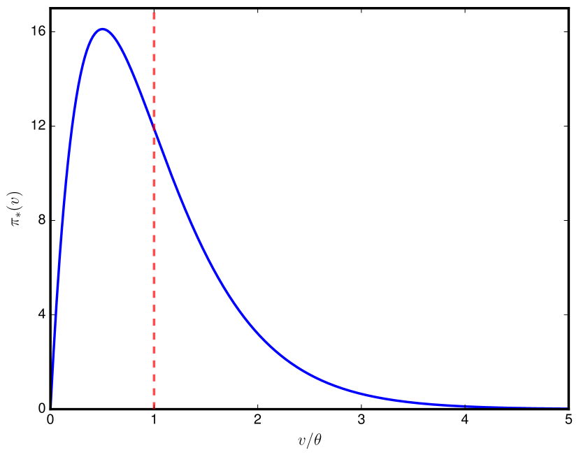
Working with probability densities and their corresponding partial differential equations allows for a greater flexibility concerning the choice of initial conditions. For stochastic differential equations restricting the variance $v=v_{0}$ to a certain initial value $v_{0}$ at $t=0$ is the usual choice even though, in contrast to the returns $x_{t}$, we do not know the precise value $v_{0}$ of $v_{t}$ at $t=0$. The choice of a random $v_{0}$ with distribution $\pi_{\ast}$ is more sensible because variance is stationary distributed if Heston’s model holds true for stock markets. Dealing with those initial conditions is barely possible within the SDE frame but setting

$$p(x_{0},v_{0})=\delta(x_{0})\pi_{\ast}(v_{0})$$ (2.7)

as initial condition for the joint probability density subject to the PDE Eq. (2.3) is no problem at all and is adopted for our numerical simulation of the PDE Eq. (2.3). Since the PDE Eq. (2.3) is linear, any linear combination of solutions is a solution as well. If $p(x_{t},v_{t}|v_{0})$ denotes a solution for the initial condition Eq. (2.4), the weighted average

$$\int dv_{0}\,p(x_{t},v_{t}|v_{0})\pi_{\ast}(v_{0})$$

is a solution of the PDE Eq. (2.3) as well with initial value

$$\int dv_{0}\,p(x_{0},v|v_{0})\pi_{\ast}(v_{0})=\int dv_{0}\,\delta(x_{0})\delta(v-v_{0})\pi_{\ast}(v_{0})=\delta(x_{0})\pi_{\ast}(v_{0})\,.$$

Hence, solving the PDE Eq. (2.3) for the initial condition Eq. (2.7) yields as solution the weighted average of all solutions with known initial variance $v_{0}$.

2.2 Solving the Fokker-Planck equation

There exists an analytical solution of the Fokker-Planck equation Eq. (2.3) in form of Fourier and inverse Laplace transforms which we shortly derive following [15]. First, we take the Fourier transform.

$$p(x_{t},v_{t}|v_{0})=\int_{-\infty}^{\infty}\dfrac{dp_{x}}{2\pi}\exp(ip_{x}x_{t})\bar{p}_{p_{x}}(v_{t}|v_{0})\,,$$

i.e., $\bar{p}_{p_{x}}(v_{t}|v_{0})$ is the Fourier transform of $p(x_{t},v_{t}|v_{0})$ w.r.t. $x_{t}$. Second, the Laplace transform

$$\tilde{p}_{t,p_{x}}(p_{v}|v_{0})=\int_{0}^{\infty}dv\exp(-p_{v}v)\bar{p}_{p_{x}}(v_{t}=v|v_{0})\,.$$ (2.8)

solves the partial differential equation of first order

$$\left[\partial_{t}+\left(\Gamma p_{v}+\dfrac{\kappa^{2}}{2}p_{v}^{2}-\dfrac{p_{x}^{2}-ip_{x}}{2}\right)\partial_{p_{v}}\right]\tilde{p}=-\gamma\theta p_{v}\tilde{p}$$

where we introduced the notation

$$\Gamma=\gamma+i\rho\kappa p_{x}\,.$$

This PDE has to be solved with initial condition

$$\tilde{p}_{t=0,p_{x}}(p_{v}|v_{0})=\exp(-p_{v}v_{0})\,.$$

The solution of this initial problem is given by the method of characteristics

$$\tilde{p}_{t,p_{x}}(p_{v}|v_{0})=\exp\left(-\tilde{p}_{v}(0)v_{0}-\gamma\theta\int_{0}^{t}d\tau\,\tilde{p}_{v}(\tau)\right)\,$$

where the function $\tilde{p}_{v}(\tau)$ is the solution of the characteristic (ordinary) differential equation

$$\dfrac{\tilde{p}_{v}(\tau)}{d\tau}=\Gamma\tilde{p}_{v}(\tau)+\dfrac{\kappa^{2}}{2}\tilde{p}_{v}^{2}(\tau)-\dfrac{p_{x}^{2}-\text{i}p_{x}}{2}$$

with the boundary condition $\tilde{p}_{v}(t)=p_{v}$ specified at $\tau=t$. The differential equation is of the Riccati type with constant coefficients, and its solution is

$$\tilde{p}_{v}(\tau)=\dfrac{2\Omega}{\kappa^{2}}\left(\zeta e^{\Omega(t-\tau)}-1\right)^{-1}-\dfrac{\Gamma-\Omega}{\kappa^{2}}\,,$$

where we introduced the frequency

$$\Omega=\sqrt{\Gamma^{2}+\kappa^{2}(p_{x}^{2}-\text{i}p_{x})}$$

and the coefficient

$$\zeta=1+\dfrac{2\Omega}{\kappa^{2}p_{v}+(\Gamma-\Omega)}\,.$$

Substituting yields

$$\tilde{p}_{t,p_{x}}(p_{v}|v_{0})=\exp\left(-\tilde{p}_{v}(0)v_{0}+\dfrac{\alpha(\Gamma-\Omega)t}{2}-\alpha\log\dfrac{\zeta-e^{-\Omega t}}{\zeta-1}\right)\,$$ (2.9)

with $\alpha$ defined in Eq. (2.6). Since we are interested in a solution of the Fokker-Planck equation w.r.t. to the initial conditions Eq. (2.7) we take the average of all solution Eq. (2.9) with weight $\pi_{\ast}(v_{0})$ and obtain

$$\tilde{p}_{t,p_{x}}(p_{v}) =\int_{0}^{\infty}dv_{0}\,\tilde{p}_{t,p_{x}}(p_{v}|v_{0})\pi(v_{0})$$

$$=\left(1+\dfrac{\theta\tilde{p}_{v}(0)}{\alpha}\right)^{\alpha}\left(\dfrac{\zeta-e^{-\Omega t}}{\zeta-1}\right)^{\alpha}\exp\left(\dfrac{\alpha(\Gamma-\Omega)t}{2}\right)\,.$$ (2.10)

The solution $p(x_{t},v_{t})$ of Eq. (2.3) with initial condition Eq. (2.7) can be efficiently computed from Eq. (2.2) applying the Stehfest method of degree $12$ – see [1] – to compute the inverse of the Laplace transform Eq. (2.8). This procedure performs magnitudes faster than solving the Fokker-Planck equation itself numerically, a method we tested also in order to validate our numerical findings by two unrelated computational approaches. Beside the joint distribution $p(x_{t},v_{t})$ we also need the conditional distribution

$$p(x_{t}|v_{0})=\int_{0}^{\infty}dv_{t}\,p(x_{t},v_{t}|v_{0})$$

which is the marginal distribution of the joint density $p(x_{t},v_{t}|v_{0})$, that is, the solution of the Fokker-Planck equation Eq. (2.3) w.r.t. the initial conditions Eq. (2.4). There is a Fourier transform representation of the conditional density [15]

$$p(x_{t}|v_{0})=\int_{-\infty}^{\infty}\dfrac{dp_{x}}{2\pi} \exp\left(\text{i}p_{x}x-\dfrac{p_{x}^{2}-\text{i}p_{x}}{\Gamma+\Omega\coth(\Omega t/2)}\right)$$

$$\times \exp\left(-\dfrac{2\gamma\theta}{\kappa^{2}}\log\left(\cosh\dfrac{\Omega t}{2}+\dfrac{\Gamma}{\Omega}\sinh\dfrac{\Omega t}{2}\right)+\dfrac{\gamma\Gamma\theta t}{\kappa^{2}}\right)\,$$ (2.11)

and the density of the marginal distribution of the returns [15]

$$p(x_{t})=\int_{-\infty}^{\infty}\dfrac{dp_{x}}{2\pi}\exp\left(\text{i}p_{x}x+\dfrac{\gamma\theta}{\kappa^{2}}\Gamma t-\dfrac{2\gamma\theta}{\kappa^{2}}\log\left(\cosh\dfrac{\Omega t}{2}+\dfrac{\Omega^{2}-\Gamma^{2}+2\gamma\Gamma}{2\gamma\Omega}\sinh\dfrac{\Omega t}{2}\right)\right)\,.$$ (2.12)

Knowledge of $p(x_{t}|v_{0})$ and $p(x_{t})$ allows for a numerical computation of the informational flow Eq. (3.2) via lemma 3.2 and of the mutual information $I(S_{(n+1)\tau}:S_{n\tau})$. All simulations are done with Python using Numpy [43].

3 Information Theory

3.1 Mutual Information

The differential entropy $h(X)$ of a continuous random real-variable $X$ with density $f(x)$ is defined as [11]

$$h(X)=-\int f(x)\log f(x)\,dx\,$$

if it exists, that is, the previous integral does not diverge. Since we measure information in bits we use the logarithm w.r.t. base $2$. In contrast to the discrete case, there is no canonical definition as one has to choose a reference measure $dx$ w.r.t. which the density is integrated. In the sequel we assume existence of the integrals without mentioning it. Further, we assume that the Lebesgue measure is chosen as reference. Compared to entropy of discrete random variables, differential entropy can be negative. One example provides a normally distributed random variable $X\sim(1/\sqrt{2\pi\sigma^{2}})\exp(-x^{2}/2\sigma^{2})$ whose differential entropy is $1/2\log(2\pi e\sigma^{2})$ [11] which can be negative for sufficiently small variances $\sigma^{2}$. Even though it might become negative, the differential entropy, as the entropy of discrete random variables, can be interpreted as a measure of the average uncertainty in the random variable. The differential entropy behaves nicely under diffeomorphic coordinate changes $\phi:S_{X}\rightarrow\mathbb{R}$ on the support $S_{X}=\{x:f(x)>0\}\subseteq\mathbb{R}$ of the random variable $X$

$$h(\phi(X))=h(X)+\int f(x)\log|\phi^{\prime}(x)|\,dx$$

The differential entropy of a set $X_{1},X_{2},\ldots,X_{n}$ of random variables with joint density $f(x_{1},x_{2},$ $\ldots,x_{n})$ is defined as

$$h(X_{1},X_{2},\ldots,X_{n})=-\int f(x_{1},x_{2},\ldots,x_{n})\log f(x_{1},x_{2},\ldots,x_{n})\,dx_{1}dx_{2}\cdots dx_{n}\,.$$

For every differeomophism $\phi:S_{\mathbf{X}}\rightarrow\mathbb{R}^{n}$ on the support $S_{\mathbf{X}}=\{\mathbf{x}=(x_{1},x_{2},\ldots,x_{n}):\,f(x_{1},x_{2},\ldots,x_{n})>0\}$ of the random variables $\mathbf{X}=(X_{1},X_{2},\ldots,X_{n})$ we obtain

$$h(\phi(\mathbf{X}))=h(\mathbf{X})+\int f(\mathbf{x})\log|\det J_{\phi}(\mathbf{x})|\,d\mathbf{x}$$

where $J_{\phi}(\mathbf{x})$ is the Jacobian of $\phi$.
If the random variables $X,Y$ have a joint density function $f(x,y)$ and conditional density function $f(x|y)$, respectively, we can define the conditional entropy $h(X|Y)$ as

$$h(X|Y)=-\int f(x,y)\log f(x|y)\,dxdy\,.$$

Since in general $f(x|y)=f(x,y)/f(y)$, we can also write

$$h(X|Y)=h(X,Y)-h(Y)\,.$$

But we must be careful if any of the differential entropies are infinite. $h(X|Y)$ is a measure of the average uncertainty of the random variable $X$ conditional on the knowledge of another random variable $Y$.
The relative entropy (or Kullback Leibler divergence) $D(f||g)$ between two densities $f$ and $g$ is defined by

$$D(f||g)=\int f(x)\log\dfrac{f(x)}{g(x)}\,dx.$$

Note that $D(f||g)$ is finite only if the support set $\{x:f(x)>0\}$ of $f$ is contained in the support of $g$ (Motivated by continuity, we set $0\log(0/0)=0$.). While $D(f||g)$ is in general not symmetric, it is often considered as a kind of distance between $f$ and $g$. This is mainly due to its property that $D(f||g)\geq 0$ with equality if and only if $f=g$.
The mutual information $I(X:Y)$ between two random variables $X$ and $Y$ with joint density $f(x,y)$ and respective marginal densities $g(x)$ and $k(y)$ is defined as

$$I(X:Y) = h(X)-h(X|Y)$$

$$= h(Y)-h(Y|X)$$

$$= h(X)+h(Y)-h(X,Y)$$

$$= \int f(x,y)\log\dfrac{f(x,y)}{g(x)k(y)}\,dxdy$$

$$= D(f(x,y)||g(x)k(y))\,.$$

Again, we must be careful if any of the differential entropies are infinite and the mutual information might or might not diverge in this case.
From the definition it is clear that the mutual information is symmetric, i.e., $I(X:Y)=I(Y:X)$. Further, $I(X:Y)\geq 0$ with equality if and only if $X$ and $Y$ are independent. Thus, mutual information can be considered as a general measure of statistical dependence as it detects any deviations of independence. Note that in the case of independence, knowledge of $X$ does not reduce our uncertainty about $Y$, i.e., $X$ provides no information about $Y$, and vice versa.
Like mutual information, conditional mutual information $I(X:Y|Z)$ between three random variables $X,Y$ and $Z$ can be written in terms of conditional entropies as

$$I(X:Y|Z)=h(X|Z)-h(X|Y,Z)$$

assuming the differential entropies exist. This can be rewritten to show its relationship to mutual information

$$I(X:Y|Z)=I(X:Y,Z)-I(X:Z)$$

usually rearranged as the chain rule of mutual information [11]

$$I(X:Y,Z)=I(X:Y|Z)+I(X:Z)\,.$$ (3.1)

In contrast to differential entropy, mutual information and conditional mutual information are scaling invariant, that is, for three diffeomorphic maps $\phi_{X},\phi_{Y},\phi_{Z}:\mathbb{R}\rightarrow\mathbb{R}$ we have [26]

$$I(\phi_{X}(X):\phi_{Y}(Y) )=I(X:Y)$$

$$I(\phi_{X}(X):\phi_{Y}(Y) |\phi_{Z}(Z))=I(X:Y|Z).$$

In the last section we defined

$$x_{t} =\log(S_{t}/S_{0})-\mu t$$

$$v_{t} =\sigma^{2}_{t}\,.$$

Both transformations are diffeomorphic on the support of the respective random variables. Scaling invariance of the mutual information yields

Lemma 3.1.

The mutual information between stock and volatility is the same as the one between adjusted log-returns and variance.

$$I(\sigma_{t}:S_{t})=I(v_{t}:x_{t})$$

3.2 Multilevel Dynamical Systems

We consider the process $t\rightarrow(S_{t},\sigma_{t})$ with a fixed initial value $S_{0}$, the stock price today, and a stationary distributed volatility $\sigma_{0}$. Since volatility is a hidden parameter, the only observable is the stock $S_{t}$. Then, we discretize the continuous processes $S_{t}$ and $\sigma_{t}$ in time with resolution $\tau$. This is sensible because the observable, that is, stock data, is in general only quoted at discrete time points, most commonly at the end of every trading day, i.e., $\tau=1$ day. From this we obtain a Markov process in discrete time $n\rightarrow(S_{n\tau},\sigma_{n\tau})$. Since only the stock price can be observed, we can illustrate the situation as in Fig. (2) with $\phi$ being the observation map that simply projects onto its first component.

Figure 2: Basic setup of a low level process that can be observed via an observation map $\phi$.

We investigate to which extend the observed process $n\rightarrow S_{n\tau}$ is a stochastic process in its own right. The dashed line on the upper level indicates that the upper process is not self-contained, because $S_{(n+1)\tau}$ cannot in general be derived from $S_{n\tau}$ solely, whereas the solid line on the lower level indicates the Markovian dynamics for the stochastic differentials for $S_{n\tau}$ and $\sigma_{n\tau}$ or, equivalently, $x_{n\tau}$ and $v_{n\tau}$ via Eq. (2.2). Such multilevel dynamical systems are extensively studied in [36] where we introduced various information theoretical measures in order to make the notion “self-contained” precise and the deviation of a process from being self-contained quantifiable. Two of them are of particular interest.
Informational closure: We called the higher process to be informationally closed, if there is no information flow from the lower to the higher level. Knowledge of the joint state $(S_{n\tau},\sigma_{n\tau})$ will not improve predictions of the stock $S_{(n+1)\tau}$ at time $n+1$ when $S_{n\tau}$ is already known, i.e., for $S_{(n+1)\tau}=\phi(S_{(n+1)\tau},\sigma_{(n+1)\tau})$ we have

$$I(S_{(n+1)\tau}:(S_{n\tau},\sigma_{n\tau})|S_{n\tau})=0\,.$$ (3.2)

Markovianity: Markovianity of the upper process $n\rightarrow S_{n\tau}$ is another property that allows to be considered a self-contained process in its own right. In this case $S_{(n+1)\tau}$ is independent of the entire past trajectory

$${\bf S}^{\tau}_{n-1}=(S_{(n-1)\tau},\ldots,S_{\tau},S_{0})\,$$

given $S_{n\tau}$, which can be expressed again in terms of the conditional mutual information as

$$I(S_{(n+1)\tau}:{\bf S}^{\tau}_{n-1}|S_{n\tau})=0\,.$$ (3.3)

In our setting, i.e., with $S_{t}$ and $\sigma_{t}$ derived from Heston’s model with initial condition Eq. (2.4) and then discretized according to Fig. (2) we obtain the following results:

Lemma 3.2.

The information flow can be computed as

$$I(S_{(n+1)\tau}:(S_{n\tau},\sigma_{n\tau})|S_{n\tau})=I(x_{(n+1)\tau}:v_{n\tau}|x_{n\tau})$$

for all $\tau>0$ and $n\in\mathbb{N}$.

Proof.

Lemma 3.1 implies

$$I(S_{(n+1)\tau}:(S_{n\tau},\sigma_{n\tau})|S_{n\tau})=I(x_{(n+1)\tau}:(x_{n\tau},v_{n\tau})|x_{n\tau})$$

Then, by the chain rule of mutual information Eq. (3.1) this can be expanded as

$$I(x_{(n+1)\tau}:(x_{n\tau},v_{n\tau})|x_{n\tau})=I(x_{(n+1)\tau}:v_{n\tau}|x_{n\tau})+I(x_{(n+1)\tau}:x_{n\tau}|x_{n\tau},v_{n\tau})\,.$$

The result then follows from $I(x_{(n+1)\tau}:x_{n\tau}|x_{n\tau},v_{n\tau})=0$. ∎

As a corollary, for the first step, i.e., $n=0$ we obtain

Corollary 3.3.

$$I(S_{\tau}:(S_{0},\sigma_{0})|S_{0})=I(x_{\tau}:v_{0})$$

from lemma 3.2 and by dropping the implicit condition $x_{0}=0$. Similarly, we can derive a bound on the deviation from Markovianity for the stock process $n\rightarrow S_{n\tau}$ based on the information flow.

Theorem 3.4.

In the setting of Fig. (2)

$$I(S_{(n+1)\tau}:{\bf S}^{\tau}_{n-1}|S_{n\tau})\leq I(x_{(n+1)\tau}:v_{n\tau}|x_{n\tau})\,.$$

for all $\tau>0$ and $n\in\mathbb{N}$.

Proof.

Scale invariance and decomposing the mutual information yields

$$I(S_{(n+1)\tau}:{\bf S}^{\tau}_{n-1}|S_{n\tau})= I(x_{(n+1)\tau}:{\bf x}^{\tau}_{n-1}|x_{n\tau})$$

$$\leq I(x_{(n+1)\tau}:({\bf x}^{\tau}_{n-1},v_{n\tau})|x_{n\tau})$$

$$= I(x_{(n+1)\tau}:v_{n\tau}|x_{n\tau})+I(x_{(n+1)\tau}:{\bf x}^{\tau}_{n-1}|x_{n\tau},v_{n\tau})$$

Markovianity of the process $n\rightarrow(x_{n\tau},v_{n\tau})$ yields $I(x_{(n+1)\tau}:{\bf x}^{\tau}_{n-1}|x_{n\tau},v_{n\tau})=0$. ∎

4 Inferring volatility from stock data

4.1 Information in the Heston Model

As an example for our numerical studies we take realistic parameters from [2] where Heston’s model was fitted directly on the S&P 500 and its VIX. They got the values

$$\gamma=5.07,\,\theta=0.0457,\kappa=0.48,\rho=-0.767$$ (4.1)

The VIX is quoted in percentage points and translates, roughly, to the expected movement (with the assumption of a 68% likelihood, i.e., one standard deviation) in the S&P 500 index over the next 30-day period, which is then annualized. Hence, the solution of the PDE Eq. (2.9) with these parameters and initial condition Eq. (2.7) until $t=2.0$ corresponds to two years, that is, $554$ trading days.

Figure 3: The evolution of the mutual information $I(\sigma_{t}:S_{t})$ for the joint distribution $p(x_{t},v_{t})$ solving the PDE Eq. (2.3) with initial condition Eq. (2.7). The maximum is approximately at $t=55$ trading days.

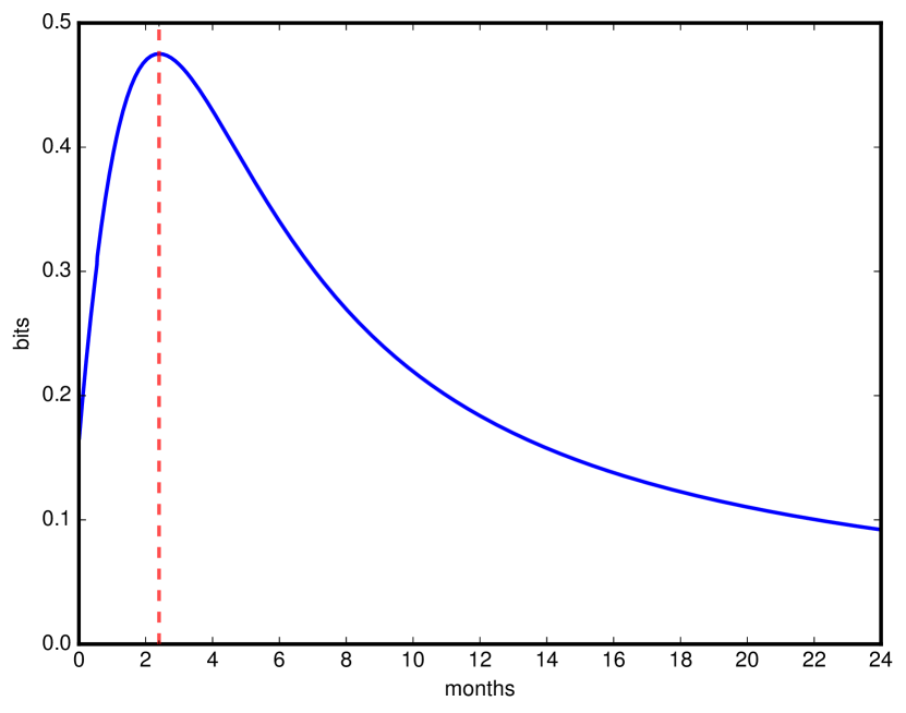
Originally, we computed the mutual information $I(v_{t}:x_{t})$ but due to lemma 3.1 we have $I(\sigma_{t}:S_{t})=I(v_{t}:x_{t})$. One can read off Fig. (3) three remarkable facts. First, the maximum $I(\sigma_{\tau}:S_{\tau})=0.48$ bits at $\tau=55$ trading days. Second, the mutual information diminishes for longer times $t$. Third, and most important, the small amount of information left in the stock about its underlying volatility. We get at most about half a bit which makes at least $25$ independent measurements necessary to derive $10$ bits, that is about three digits of the volatility. We could possibly obtain more information by observing multiple successive stock prices $S_{t},S_{t-1},\ldots$, but due to the stochasticity of the volatility process the information is still rather limited. Below, we illustrate this effect in the case of stochastic volatility models based on Gaussian processes. Third, the instantaneous jump of the mutual information $I(v_{t}:x_{t})$ for $t\rightarrow 0$. Since the distributions of the adjusted log-return $x_{t}$ and the variance $v_{t}$ are chosen to be independent at $t=0$, see Eq. (2.7), mutual information $I(x_{0}:v_{0})=0$. But the numerical simulation suggest the limit $\lim_{t\rightarrow 0}I(x_{t}:v_{t})\approx 0.166$ bits.
Next, we compute the informational flow.

$$I(S_{(n+1)\tau}:(S_{n\tau},\sigma_{n\tau})|S_{n\tau})=I(S_{(n+1)\tau}:\sigma_{n\tau}|S_{n\tau})$$

Lemma 3.2 yields

$$I(S_{(n+1)\tau}:\sigma_{n\tau}|S_{n\tau}) =I(x_{(n+1)\tau}:v_{n\tau}|x_{n\tau})$$

$$=h(x_{(n+1)\tau}|x_{n\tau})-h(x_{(n+1)\tau}|x_{n\tau},v_{n\tau})$$

$$=h(x_{(n+1)\tau},x_{n\tau})-h(x_{n\tau})-h(x_{\tau}|x_{0},v_{0})\,$$ (4.2)

where the last equality follows from $p(x_{(n+1)\tau}|x_{n\tau},v_{n\tau})=p(x_{\tau}|x_{0},v_{0})$, i.e., the temporal homogeneity of solutions of the Fokker-Planck equation Eq. (2.3). The conditional distribution $p(x_{\tau}|x_{0},v_{0})$ is in general not equal (2.2) as long as the condition on $x_{0}$ is replaced by $x_{0}=0$. If $x_{0}=x$, then

$$h(x_{\tau}|x_{0},v_{0})=-\int p(x_{\tau}=y|x_{0}=x,v_{0})\log p(x_{\tau}=y|x_{0}=x,v_{0})\,dy$$

If we change the coordinates $y^{\prime}=y-x$ and $x^{\prime}=x$, the Jacobian of this coordinate transformation is $1$ and we obtain

$$h(x_{\tau}|x_{0},v_{0})=-\int p(x_{\tau}=y^{\prime}+x^{\prime}|x_{0}=x^{\prime},v_{0})\log p(x_{\tau}=y^{\prime}+x^{\prime}|x_{0}=x^{\prime},v_{0})\,dy^{\prime}$$

Since solutions $(x_{t},v_{t},x_{0},v_{0})\mapsto p(x_{t},v_{t}|x_{0},v_{0})$ of the PDE Eq. (2.3) depend only on $(x_{t}-x_{0},v_{t},0,v_{0})$, we obtain $p(x_{\tau}=y^{\prime}+x^{\prime}|x_{0}=x^{\prime},v_{0})=p(x_{\tau}=y^{\prime}|x_{0}=0,v_{0})$. This implies $h(x_{\tau}|x_{0},v_{0})=h(x_{\tau}|v_{0})$ adopting the rule that we drop the implicit condition $x_{0}=0$. Hence, the entropy $h(x_{\tau}|x_{0},v_{0})$ is the one of the conditional density Eq. (2.2).
Computing the joint density $p(x_{((n+1)\tau},x_{n\tau})$ yields

$$p(x_{(n+1)\tau},x_{n\tau}) =\int p(x_{(n+1)\tau},x_{n\tau},v_{n\tau}=v)dv$$

$$=\int p(x_{(n+1)\tau}|x_{n\tau},v_{n\tau}=v)p(x_{n\tau},v_{n\tau}=v)dv$$

$$=\int p(x_{\tau}|x_{0},v_{0}=v)p(x_{n\tau},v_{n\tau}=v)dv\,.$$

Its entropy reads

$$h(x_{(n+1)\tau},x_{n\tau}) =-\int p(x_{(n+1)\tau}=y,x_{n\tau}=x)\log p(x_{(n+1)\tau}=y,x_{n\tau}=x)\,dxdy$$

$$=-\int\bigg{(}\int p(x_{\tau}=y|x_{0}=x,v_{0}=v)p(x_{n\tau}=x,v_{n\tau}=v)dv\bigg{)}$$

$$\quad\times\log\bigg{(}\int p(x_{\tau}=y|x_{0}=x,v_{0}=v)p(x_{n\tau}=x,v_{n\tau}=v)dv\bigg{)}\,dxdy\,.$$

Furthermore, changing coordinates $y^{\prime}=y-x$ and $x^{\prime}=x$ yields

$$h(x_{(n+1)\tau} ,x_{n\tau})=$$

$$- \int\bigg{(}\int p(x_{\tau}=y^{\prime}+x^{\prime}|x_{0}=x^{\prime},v_{0}=v)p(x_{n\tau}=x^{\prime},v_{n\tau}=v)dv\bigg{)}$$

$$\times\log\bigg{(}\int p(x_{\tau}=y^{\prime}+x^{\prime}|x_{0}=x^{\prime},v_{0}=v)p(x_{n\tau}=x^{\prime},v_{n\tau}=v)dv\bigg{)}\,dx^{\prime}dy^{\prime}\,.$$

We substitute $p(x_{\tau}=y^{\prime}+x^{\prime}|x_{0}=x^{\prime},v_{0}=v)=p(x_{\tau}=y^{\prime}|x_{0}=0,v_{0}=v)$ and reduced Eq. (4.1) to expressions which can be computed via Eq. (2.2) and Eq. (2.9), at least numerically. We simulated the informational flow Eq. (3.2) for several choices of $n$.
Beside the informational flow, we are also interested in the mutual information $I(S_{(n+1)\tau}:S_{n\tau})=I(x_{(n+1)\tau}:x_{n\tau})$ between two subsequent observations of the stock. Definition of the conditional mutual information yields

$$I(x_{(n+1)\tau}:v_{n\tau}|x_{n\tau}) =I(x_{(n+1)\tau}:v_{n\tau},x_{n\tau})-I(x_{(n+1)\tau}:x_{n\tau})$$

$$=h(x_{(n+1)\tau})-h(x_{(n+1)\tau}|v_{n\tau},x_{n\tau})-I(x_{(n+1)\tau}:x_{n\tau})$$

$$=h(x_{(n+1)\tau})-h(x_{\tau}|v_{0},x_{0})-I(x_{(n+1)\tau}:x_{n\tau})$$

$$=h(x_{(n+1)\tau})-h(x_{\tau}|v_{0})-I(x_{(n+1)\tau}:x_{n\tau})$$

where the last equation follows from the previously proven identity $h(x_{\tau}|v_{0},x_{0})=h(x_{\tau}|v_{0})$ where the last entropy is the one of the conditional distribution Eq. (2.2). The entropy $h(x_{(n+1)\tau})$ can be computed via formula Eq. (2.12) for the density of $x_{t}$. Hence,

$$I(S_{(n+1)\tau}:S_{n\tau})=I(x_{(n+1)\tau}:x_{n\tau})=h(x_{(n+1)\tau})-h(x_{\tau}|v_{0})-I(x_{(n+1)\tau}:v_{n\tau}|x_{n\tau})\,.$$ (4.3)

In particular, if we set $n=0$ we obtain $I(S_{\tau}:S_{0})=0$. For the other values of $n$ we plotted Fig. (5) the ratio

$$\dfrac{I(S_{(n+1)\tau}:\sigma_{n\tau}|S_{n\tau})}{I(S_{(n+1)\tau}:S_{n\tau})}$$ (4.4)

which expresses the informational gain on predictions of future stock movements $S_{(n+1)\tau}$ we obtain from knowing the instantaneous volatility compared to the information already there from reading off stock data $S_{n\tau}$ at time $n\tau$.

Figure 4: The informational flow $I(S_{(n+1)\tau}:\sigma_{n\tau}|S_{n\tau})$ for $n=0,1,2,4,6,10$, and $15$.

Figure 5: The ratio $I(S_{(n+1)\tau}:\sigma_{n\tau}|S_{n\tau})/I(S_{(n+1)\tau}:S_{n\tau})$ for $n=1,2,4,6,10$, and $15$.

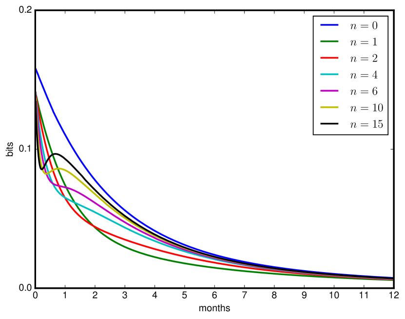
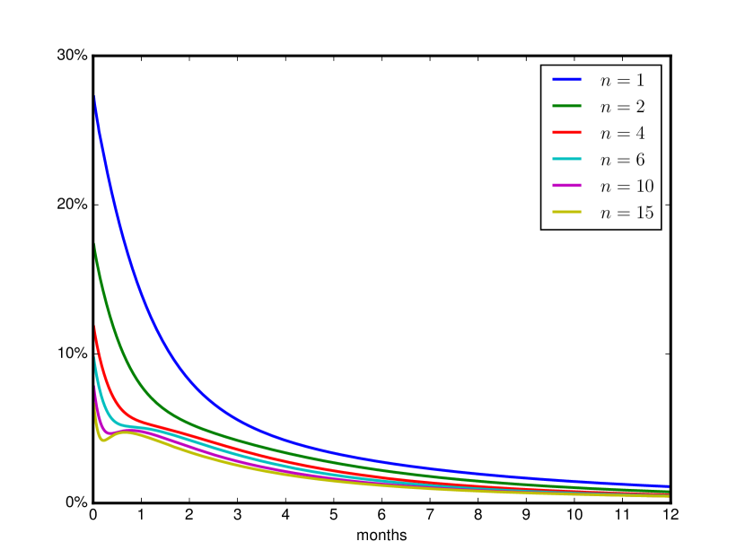
Several facts can be read off Fig. (4) and Fig. (5). First, the informational flow $I(S_{\tau}:\sigma_{0}|S_{0})=I(x_{\tau}:v_{0})$ is an upper bound of the general flow $I(S_{(n+1)\tau}:\sigma_{n\tau}|S_{n\tau})=I(x_{(n+1)\tau}:v_{n\tau}|x_{n\tau})$ for all $n\in\mathbb{N}_{0}$. Second, the incredible small amount of this flow: the knowledge of the joint state $(S_{n\tau},\sigma_{n\tau})$ will not remarkably improve predictions on the stock $S_{(n+1)\tau}$ at time $\tau$ if $S_{n\tau}$ is already known. The informational gain $I(S_{(n+1)\tau}:\sigma_{n\tau}|S_{n\tau})$ compared to the information $I(S_{(n+1)\tau}:S_{n\tau})$ we already have about $S_{(n+1)\tau}$ if we read off $S_{n\tau}$ is at most $27\%$ and vanishes if $\tau$ or $n$ increases. Diminishing informational gain on future returns from knowing the instantaneous volatility $v_{n\tau}$ if $n$ grows can be directly derived from Eq. (4.3): we already know from Fig. (4) that $I(S_{(n+1)\tau}:\sigma_{n\tau}|S_{n\tau})$ is upper bounded by $I(S_{\tau}:\sigma_{0}|S_{0})=h(x_{\tau})-h(x_{\tau}|v_{0})$ independent of $n$ whereas $h(x_{(n+1)\tau})$ is extensive in $n$ because the marginal distribution of $x_{(n+1)\tau}$ is roughly Gaussian with a variance proportional to $(n+1)\tau$. Hence, $h(x_{(n+1)\tau})\approx\mathcal{O}\left(\log\left((n+1)\tau\right)\right)$. The same argument yields $h(x_{\tau}|v_{0})\approx\mathcal{O}(\log\left(\tau)\right)$ and therefore

$$I(S_{(n+1)\tau}:S_{n\tau})=I(x_{(n+1)\tau}:x_{n\tau})\approx\log\left((n+1)\tau\right)-\log\tau=\log(n+1)\,,$$

that is, the denominator in Eq. (4.4) grows logarithmically in $n$. Overall, knowing the instantaneous volatility $\sigma_{n\tau}$ does not deliver considerably better estimations on future stock-returns than the knowledge of the stationary distribution $\pi_{\ast}(\sigma_{n})$ of the volatility does, which we know already from the model. Therefore, inferring the realized volatility from market data in financial markets subject to Heston’s model is not only hard, but also of limited value when predicting prices. Third, from theorem 3.4 follows that the stock process $S_{n\tau}\rightarrow S_{(n+1)\tau}$ is nearly Markovian for increasing $\tau$. Last, also the informational flow $I(S_{(n+1)\tau}:\sigma_{n\tau}|S_{n\tau})$ makes an instantaneous jump for $\tau\rightarrow 0$ with the same jump height for $n=0$ as the mutual information $I(x_{\tau}:v_{\tau})$ in Fig. (3).
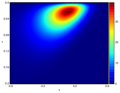
Finally, we investigate in this subsection the influence of the parameters $\rho$ on the mutual information $I(\sigma_{t},S_{t})$. Recall, $\rho$ is the instantaneous correlation between the two Brownian motions $W^{(1)}_{t}$ and $W^{(2)}_{t}$ driving the processes $S_{t}$ and $v_{t}$, respectively. $\rho$ is negative to capture the leverage effect [6], i.e., negative returns tend to increase volatility. The effect on the joint probability is nicely captured by figure Fig. (6). The joint distribution of the first figure is skewed towards negative returns if volatility increases whereas the second presents a nearly symmetric distribution, i.e., negative returns affect volatility not more than positive ones.

Leverage Effect Included	Leverage Effect Excluded

Figure 6: The joint distribution $p(x_{\tau},v_{\tau})$ of the Heston process with parameters as in Eq. (4.1) for $\tau=252$ trading days. If $\rho=-0.767$, the inclination shows the negative correlation between adjusted log-returns $x$ and variance $v$. If $\rho=0.0$ the distribution is nearly symmetric in the adjusted log returns $x$.

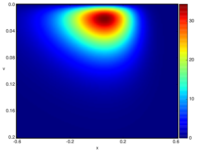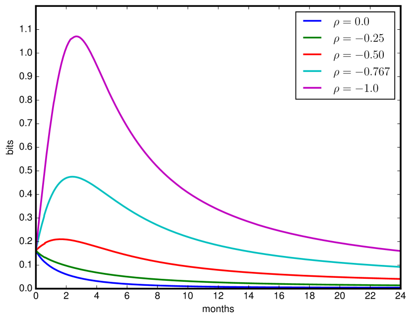
Figure Fig. (7) shows the mutual information $I(\sigma_{t}:S_{t})$ for different choices of the instantaneous correlation $\rho$. Two facts are remarkable. The growth of the information w.r.t. to $\rho$ and the negligible amount left if we choose $\rho=0.0$. In this case the stock and the volatility process are quasi independent and nearly no information about the instantaneous volatility can be obtained from stock data.

Figure 7: The evolution of the mutual information $I(\sigma_{t}:S_{t})$ for different values of the instantaneous correlation $\rho$.

4.2 Fitting Stochastic Volatility Models

The mutual information $I(S_{t}:\sigma_{t})$ quantifies the average dependence between the stock price and instantaneous volatility which we have evaluated for the Heston model above. When inferring volatility from actual stock price data we are usually less interested in the average behaviour over possible realizations of the price process $t\rightarrow S_{t}$. Rather, we want to estimate the volatility conditioned on the actual sequence of prices ${\bf S}=(S_{t_{1}},\ldots,S_{t_{n}})$ that were observed at times $t_{1}<\cdots<t_{n}$. Unfortunately, computing the full conditional distribution $p(\sigma_{t}\mid{\bf S})$ or even $p(\{\sigma_{t}\}_{t>0}:{\bf S})$ is infeasible in the Heston model. Thus, in this section we turn to a different class of models which is based on Gaussian processes. While exact inference is also infeasible in these models, Gaussian processes are heavily used in machine learning and a wide range of approximation algorithms is readily available. As described above, we consider generalizations of the exponential Ornstein-Uhlenbeck model. As before, the price process is given by

$$dS_{t}=\mu S_{t}dt+\sigma_{t}S_{t}dW_{t}^{(1)},$$

but now, the logarithm of the variance $y_{t}=\log\sigma^{2}_{t}$ is drawn from a Gaussian process. To fit such a model, we can represent the distribution of ${\bf y}=(y_{t_{1}},\ldots,y_{t_{n}})$ exactly by a multivariate Gaussian distribution. In addition, we need the likelihood of the observed prices ${\bf S}$ given ${\bf y}$, i.e., $p({\bf S}\mid{\bf y})$. Here, for simplicity, we use an Euler approximation to the stochastic differential equation for $S_{t}$ [37]:

$$S_{t+\Delta t}-S_{t}=\mu S_{t}\Delta t+\sigma_{t}S_{t}\sqrt{\Delta t}\epsilon_{t}$$

where $\epsilon_{t}\sim\mathcal{N}(0,1)$.

Thus, we assume that the observed daily return $r_{t}=\frac{S_{t+1}-S_{t}}{S_{t}}$ is drawn from a normal distribution with standard deviation $\sigma_{t}$, i.e., $r_{t}\sim\mathcal{N}(\mu,\sigma_{t})$. Since the drift of the price process is usually rather small compared to its volatility, we will assume $\mu=0$ for simplicity in the following.

In this formulation, our stochastic volatility model is a Gaussian process $y_{t}$ with a non-Gaussian likelihood model $p(r_{t}|y_{t})$. Similar models are well known and widely used in Gaussian process classification (see chapter 3 of [38]). In this context, several algorithms to approximate the posterior $p({\bf y}|{\bf r})$ have been developed. Here, we employ the Laplace approximation where the posterior is approximated by a multivariate Gaussian centred at the mode of the posterior, i.e., ${\bf y}_{\mathrm{Laplace}}=\operatorname{argmax}_{{\bf y}}p({\bf y}\mid{\bf r})=\operatorname{argmax}_{{\bf y}}\Psi({\bf y})$ where $\Psi({\bf y})=\log p({\bf r}|{\bf y})p({\bf y})$. The covariance for the approximate posterior is derived from the local curvature around the mode, i.e., $\Sigma_{\mathrm{Laplace}}^{-1}=-\nabla\nabla\log p({\bf y}_{\mathrm{Laplace}}\mid{\bf r})$.

Using the Laplace approximation it is also possible to compute an approximation to the marginal likelihood

$$p({\bf r}) = \int p({\bf r}\mid{\bf y})p({\bf y})d{\bf y}$$

$$\approx e^{\Psi({\bf y}_{\mathrm{Laplace}})}\int e^{-\frac{1}{2}({\bf y}-{\bf y}_{\mathrm{Laplace}})^{T}\Sigma_{\mathrm{Laplace}}^{-1}({\bf y}-{\bf y}_{\mathrm{Laplace}})}d{\bf y}$$

$$= p({\bf r}|{\bf y}_{\mathrm{Laplace}})p({\bf y}_{\mathrm{Laplace}})\int e^{-\frac{1}{2}({\bf y}-{\bf y}_{\mathrm{Laplace}})^{T}\Sigma_{\mathrm{Laplace}}^{-1}({\bf y}-{\bf y}_{\mathrm{Laplace}})}d{\bf y}$$

In contrast to a maximum likelihood solution, $p({\bf r})$ does not just depend on the goodness of fit, as captured by the likelihood $p({\bf r}|{\bf y}_{\mathrm{Laplace}})$. It also takes into account the prior probability $p({\bf y}_{\mathrm{Laplace}})$ as well as the uncertainty about the inferred volatility process ${\bf y}$. Thus, the marginal likelihood, automatically incorporates a trade-off between model fit and model complexity (see chapter 28 of [30] for details). For this reason, in Bayesian statistics, the marginal likelihood is often used in model selection.

Here, we use the marginal likelihood to compare different structural assumptions about the underlying volatility process. In the standard exponential stochastic volatility model $y_{t}$ is modelled as an Ornstein-Uhlenbeck process with covariance function $k^{OU}_{t,t^{\prime}}=\frac{\beta^{2}}{2\alpha}e^{-\alpha|t-t^{\prime}|}$. Here, $\frac{1}{\alpha}$ can be considered as a lengthscale as it gives the correlation time of the process. The Ornstein-Uhlenbeck process has continuous, but nowhere differentiable sample paths. In machine learning rather smooth Gaussian processes with differentiable sample paths are usually preferred. Table 1 gives some examples of popular Gaussian processes and their covariance functions.

More complex processes, combining the properties of different processes, can then for example be obtained by adding the corresponding covariance functions. In all our experiments below, we have added a bias covariance function to increase the probability to draw sample paths which are shifted away from zero. This allows our models to easily represent processes $y_{t}$ with a non-zero mean. Overall, we fit and compare processes based on the following covariance structures:

OU

Bias $+$ Ornstein-Uhlenbeck

RBF

Bias $+$ Squared exponential

RatQuad

Bias $+$ Rational quadratic

RBF_RBF

Bias $+$ Squared exponential $+$ Squared exponential

OU_OU

Bias $+$ Ornstein-Uhlenbeck $+$ Ornstein-Uhlenbeck

The model OU is just the standard exponential Ornstein-Uhlenbeck model [31], while OU_OU denotes a two-factor version of this model incorporating two independent volatility factors with different time scales. Similarly, the RBF_RBF model is a two-factor extension of the model RBF.

To fit the different models we have then optimized the kernel parameters, e.g. the lengthscale of the Ornstein-Uhlenbeck process, in order to maximize the marginal likelihood of the observed returns. Optimizations have been caried out using the Gaussian process toolbox GPy [3] with gradient descent using the Broyden–Fletcher–Goldfarb–Shanno (BFGS) algorithm from 100 different initial conditions. Using a range of different stock market data (all downloaded from Yahoo finance) we obtain results as shown in Table 2.

Our data sets cover very different time periods as well as sectors and no consistently best model can be indentified. Nevertheless, we see a preference for models including two different time scales as either RBF_RBF or OU_OU performs best, closely followed by the RatQuad kernel. The later model exhibits a power-law decay of volatility correlations which is considered as a stylized fact of stock market data. It remains to be investigated why we cannot conform this finding. Nevertheless, also the best fitting two-factor models have a long time scale implying that volatility is correlated over several weeks. In this regard our findings agree with previous results of econometric studies which strongly suggest the use of two-factor models which allow “breaking the link between tail thickness and volatility persistence” [10] as needed to fit empirical data.

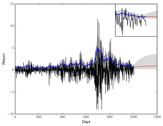
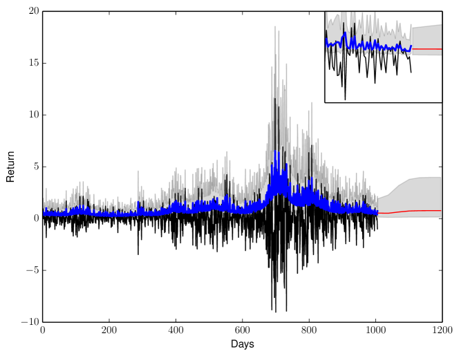
As an example, Fig. (8) shows the hidden volatility implied by the Ornstein-Uhlenbeck based (OU) as well as the best model (RBF_RBF) on the S&P 500 data. The shaded region shows the $95$% region ($\pm 2$ standard deviations from the mean) of the posterior and demonstrates the large uncertainty that remains about the volatility. When predicting the volatility for the next 100 days (red curve), the uncertainty is even more pronounced and increases quickly towards the a-priori uncertainty of the stationary volatility distribution. Note that this uncertainty is not due to parameter uncertainty which have been fixed after fitting. The situation is the same as in the Heston model were we also assumed the parameters known and the high uncertainty is due to the stochasticity of the underlying volatility process. It thus appears to be an intrinsic property of stochastic volatility models, especially if the volatility process varies quickly as in the case of realistic parameters.

Figure 8: Exponential stochastic volatility model with OU (top) and RBF_RBF (bottom) covariance function fitted to the S&P 500 data. The daily returns are shown in black with the infered volatility in blue. The grey region shows the large uncertainty ($95$% credibility region) which increases quickly when predicting into the future (red curve). The inset shows a zoom on the last 50 data points.

4.2.1 Information gain

As before, we can use information theory to quantify the amount of information obtained about the volatility. While the mutual information quantifies the average uncertainty, here we are interested in the information about ${\bf\sigma}$ that was obtained from the actually observed prices. In [13] it is suggested to consider the difference in entropy between the prior $p({\bf\sigma})$ and the posterior $p({\bf\sigma}|{\bf S})$ as the information gain from the actual prices ${\bf S}$. Thus, instead of averaging over all possible price realizations as in the conditional entropy $h({\bf\sigma}|{\bf S})$, one computes the entropy of the posterior distribution conditioned on the actually observed prices, i.e. $-\int p({\bf\sigma}|{\bf S})\log p({\bf\sigma}|{\bf S})d{\bf\sigma}$. In our case, these entropies can be evaluated since the posterior distribution $p({\bf y}|{\bf S})$ is approximated by a Gaussian and the prior $p({\bf y})$ was assumed to be a Gaussian in the first place. For a $d$-dimensional multivariate Gaussian with covariance matrix $\Sigma$ the differential entropy is given by $\frac{1}{2}\log(2\pi e)^{d}|\det\Sigma|$. To have a fair comparison with the results obtained for the Heston model, we have taken care that the uncertainty about the mean level of the volatility process did not contribute to the information gain. Thus, as in the Heston model, we assumed that the parameter specifying the stationary mean of the volatility process is known. Formally, we accomplish this by removing the bias component of the covariance function before computing the information gain. Note that the entropy of a Gaussian distribution does not depend on the mean of the distribution, and thus adjusting the mean of the prior distribution to its stationary value is not necessary when computing the information gain.

OU model	RBF_RBF model

Figure 9: Information gain about the instantaneous volatility $\sigma_{t}$ ($t=1006$) based on successively longer sequences of preceding daily returns $r_{t-\tau+1},\ldots,r_{t}$. In both models the information gain saturates after about 20 days.

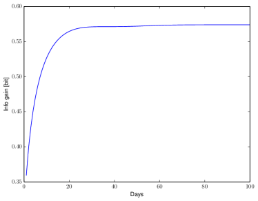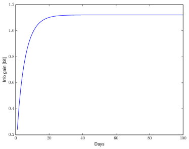
In the example shown in Fig. (8) fitted on $4$ years of data ($1006$ trading days) in total $64.5$ (OU) and $251$ bits (RBF_RBF) are obtained about the volatility ${\bf\sigma}$. The large difference reflects the fact that the OU model is less flexible and thus its a-priori uncertainty is already much smaller. Further, the results are consistent with the low information gain found for the Heston model as the above numbers correspond to just $0.06$ (OU) respectively $0.25$ (RBF_RBF) bits per observation. While this is comparable to the low values in the Heston model, especially when assuming $\rho=0$, the information about each single observation can well be larger due to the autocorrelation of the volatility process. To illustrate this effect, Fig. (9) shows the information gained about the instantaneous volatility $\sigma_{1006}$, corresponding to the last trading day in our data set, when observing the daily returns preceding it. One clearly sees that observing successive returns does reduce the uncertainty about the volatility, but after just about 20 days the information gain saturates. Thus, even observing years of data would not improve volatility estimates and just about 1 bit of information can be obtained. Again, we see that inferring volatility is notoriously hard in stochastic volatility models and volatility forecasts will be rather imprecise for quite fundamental information theoretic reasons.

Name	Covariance	Properties
Bias	1	constant sample paths
Squared Exponential	$e^{-\frac{(t-t^{\prime})^{2}}{l^{2}}}$	infinitely differentiable sample paths
Rational Quadratic	$\left(1+\frac{(t-t^{\prime})^{2}}{2\alpha l^{2}}\right)^{-\alpha}$	infinite mixture of lengthscales

Table 1: Gaussian processes that are popular in machine learning.

Description	Date	Model	log. marginal likelihood
Apple Inc.	2000-01-012003-01-01	RBF_RBF	1423.22
		RatQuad	1421.33
		OU_OU	1412.74
		OU	1412.23
		RBF	1403.32
DAX	1992-01-011995-01-01	OU_OU	2509.23
		RBF_RBF	2505.98
		RatQuad	2498.64
		RBF	2493.47
		OU	2486.51
Exxon Mobile	1986-01-011990-01-01	RBF_RBF	2923.20
		OU_OU	2921.43
		RatQuad	2906.43
		OU	2897.08
		RBF	2881.11
S&P 500	2006-01-012010-01-01	RBF_RBF	3129.78
		OU_OU	3129.58
		RatQuad	3093.42
		OU	3083.78
		RBF	3072.75

Table 2: Results of model comparison on different stock market data sets.

5 Conclusions

In this paper, we have analysed stochastic volatility models from an information theoretic perspective. In particular, we have asked how much information about the hidden volatility can be obtained from observing stock prices. First of all, the numerical results are rather surprising, at least for the authors. We have had some doubts on the information content of stocks about the volatility which is driving them in the Heston model and related stochastic volatility models, but we did not expect such a small residual value of at most $0.5$ bit for realistic parameters taken from the S&P 500. Second, mutual information $I(\sigma_{t},S_{t})$ seems to vanish in the long run or becomes at least meagre. Hence, the processes appear to be almost independent even though the adjusted log-return process $t\rightarrow x_{t}$ is entirely driven by its variance $v_{t}$, see Eq. (2.1). Third, it is not only difficult to infer the instantaneous volatility from stock data, it is mostly useless: Fig. (4) and Fig. (5) imply that knowledge of the instantaneous volatility $\sigma_{n\tau}$ just slightly improves the prediction of $S_{(n+1)\tau}$ given $S_{n\tau}$. Regarding our results in the third section, the stock process $S_{n}\rightarrow S_{(n+1)\tau}$ is almost a Markovian process in its own right. Fourth, the strong dependence of the mutual information on the instantaneous correlation $\rho$ is also surprising: again the stock and volatility processes are nearly independent if there is no correlation.
We find a similar behaviour in related stochastic volatility models which we fitted to actual stock price data. Again, we observe a large uncertainty when volatility is infered from market prices. This has severe implications for volatility forecasting and sheds doubt on the standard practice of comparing models based on their forecasting error [20]. In this case, due to uncertainty about the model parameters, forecasting should be even less precise than within a model that is perfectly specified. A possible remedy could be to incorporate option prices as well. Volatility is commonly inferred from options not from stocks. If Heston’s model holds true, what is the information between the price of an option and the volatility of the underlying stock. Furthermore, how does this value change if one increases the number of options considered? While we do not yet know the answer to these questions, it might well be that substantial uncertanties remain and volatility estimates, at least from stochastic volatility models, should be considered as unreliable for quite fundamental information theoretic reasons.

6 Funding

This work was supported by the European Research Council under the European Union’s Seventh Framework Programme (FP7/2007-2013)/ERC grant agreement no. 318723. Nils Bertschinger thanks Dr. h.c. Maucher for funding his position.

References

- [1] P. S. A. Cheng. Approximate inversion of the laplace transform. Mathematica Journal, 4(2), 1994.
- [2] Y. Aït-Sahalia and R. Kimmel. Maximum likelihood estimation of stochastic volatility models. Journal of Financial Economics, 83(2):413–452, 2007.
- [3] T. G. authors. GPy: A gaussian process framework in python. http://github.com/SheffieldML/GPy, 2012–2014.
- [4] F. Black and M. Scholes. The Pricing of Options and Corporate Liabilities. Journal of Political Economy, 81(3):637, 1973.
- [5] T. Bollerslev, J. Litvinova, and G. Tauchen. Leverage and volatility feedback effects in high-frequency data. Journal of Financial Econometrics, 4(3):353–384, 2006.
- [6] J. P. Bouchaud, a. Matacz, and M. Potters. Leverage effect in financial markets: the retarded volatility model. Physical review letters, 87(22):228701, 2001.
- [7] J.-P. Bouchaud and M. Potters. Theory of Financial Risk and Derivative Pricing. Theory of Financial Risk and Derivative Pricing, page 379, 2003.
- [8] M. Brenner and D. Galai. New financial instruments for hedging changes in volatility. Financial Analysts Journal, 45(4):61–65, 1989.
- [9] M. Brenner and D. Galai. Hedging Volatility in Foreign Currencies. The Journal of Derivatives, 1(1):53–59, 1993.
- [10] M. Chernov, A. R. Gallant, E. Ghysels, and G. Tauchen. Alternative models of stock price dynamics. Journal of Econometrics, 116:225–257, 2003.
- [11] T. M. Cover and J. A. Thomas. Elements of Information Theory. Wiley-Interscience, 2 edition, July 2006.
- [12] K. S. D. Duffie, J. Pan. Transform Analysis and Asset Pricing for Affine Jump-Diffusions. Econometrica, 68(6):1343–1376, 2000.
- [13] M. DeWeese and M. Meister. How to measure the information gained from one symbol. Network: Computation in Neural Systems, 10(4), 1999.
- [14] Z. Ding, C. W. Granger, and R. F. Engle. A long memory property of stock market returns and a new model. Journal of Empirical Finance, 1(1):83–106, 1993.
- [15] A. Dragulescu and V. M. Yakovenko. Probability distribution of returns in the Heston model with stochastic volatility. Quantitative Finance, 2(October):443–453, 2002.
- [16] O. Elerian, S. Chib, and N. Shephard. Likelihood inference for discretely observed non-linear diffusions. Econometrica, 69:959–993, 2001.
- [17] B. Eraker, M. Johannes, and N. G. Polson. The impact of jumps in returns and volatility. Journal of Finance, 53:1269–1300, 2003.
- [18] W. Feller. Two Singular Diffusion Problems. Annals of Mathematics, 54(2):286–295, 1951.
- [19] K. R. S. Fouque Jean-Pierre, George Papanicolaou. Mean-Reverting Stochastic Volatility. Cambridge University Press, 2000.
- [20] P. R. Hansen and A. Lunde. A forecast comparison of volatility models: does anything beat a garch(1,1)? Journal of Applied Econometrics, 20(7):873–889, 2005.
- [21] S. L. Heston. A Closed-Form Solution for Options with Stochastic Volatility with Applications to Bond and Currency Options. The Review of Financial Studies, 6(2):327–343, 1993.
- [22] J. Hull and A. White. The pricing of options on assets with stochastic volatilities. Journal of Finance, 42:281–300, 1987.
- [23] S. Hurn, K. Lindsay, and A. McClelland. Estimating the Parameters of Stochastic Volatility Models using Option Price Data. NCER Working Paper Seris, 87(October):35, 2012.
- [24] H. Johnson and D. Shanno. Option pricing when the variance is changing. Journal of Financial and Quantitative Analysis, 22:143–151, 1987.
- [25] T. H. M. Karlin S. A Second Course in Stochastic Processes. Academic Press, 1981.
- [26] A. Kraskov, H. Stögbauer, and P. Grassberger. Estimating mutual information. Phys. Rev. E, (69), 2004.
- [27] B. LeBaron. Stochastic Voltility as a Simple Generator of apparent financial power laws and long memory. Quantitative Finance, 6(1):627–631, 2001.
- [28] A. W. Lo. Long Term Memory in Stock Market Prices. Econometrica, 59(5):1279–1313, 1991.
- [29] V. Lucic. Boundary conditions for computing densities in hybrid models via PDE methods. Stochastics An International Journal of Probability and Stochastic Processes, 84(1951):705–718, 2012.
- [30] D. J. C. MacKay. Information Theory, Inference, and Learning Algorithms. Cambridge University Press, 2003. Available from http://www.inference.phy.cam.ac.uk/mackay/itila/.
- [31] J. Masoliver and J. Perello. Multiple time scales and the exponential Ornstein-Uhlenbeck stochastic volatility model. Quantitative Finance, 6:24, 2005.
- [32] J. F. Muzy, J. Delour, and E. Bacry. Modelling fluctuations of financial time series : from cascade process to stochastic volatility model. Eur. Phys. J. B, 17:537–548, 2000.
- [33] D. B. Nelson and D. P. Foster. Asymptotic filter theory for univariate arch models. Econometria, 62(1):1 – 41, 1994.
- [34] B. Øksendal. Stochastic Differential Equations. Springer, 2000.
- [35] J. Perello, R. Sircar, and J. Masoliver. Option pricing under stochastic volatility: the exponential Ornstein-Uhlenbeck model. page 26, 2008.
- [36] O. Pfante, E. Olbrich, N. Bertschinger, N. Ay, and J. Jost. Closure measures for coarse-graining of the tent map. Chaos (Woodbury, N.Y.), 24(1):013136, 2014.
- [37] P. C. B. Phillips and J. Yu. Maximum likelihood and gaussian estimation of continuous time models in finance. In T. Mikosch, J.-P. Kreiß, R. A. Davis, and T. G. Andersen, editors, Handbook of Financial Time Series, pages 497–530. Springer Berlin Heidelberg, 2009.
- [38] C. Rasmussen and C. Williams. Gaussian Processes for Machine Learning. Adaptive Computation and Machine Learning. MIT Press, Cambridge, MA, USA, Jan. 2006.
- [39] C. Shannon. A mathematical theory of communication. The Bell System Technical Journal, 27:379–423, 1948.
- [40] N. Shepard. Stochastic Volatility: Selected Readings. Oxford University Press, 1 edition, March 2005.
- [41] S. Shreve. Stochastic Calculus for Finance II. Number 3. Springer, 2004.
- [42] S. J. Taylor. Financial returns modelled by the product of two stochastic processes — a study of daily sugar prices 1961-79. Time Series Analysis: Theory and Practice, 1:203–226, 1982.
- [43] S. van der Walt, C. S. Colbert, and G. Varoquaux. The numpy array: A structure for efficient numerical computation. Computing in Science & Engineering, 13:22–30, 2011.