A Simple Parallel Algorithm with an O(1/t)𝑂1𝑡O(1/t) Convergence Rate for General Convex Programsthanks: Using the methodology initiated in the current paper, we further developed a different primal-dual type algorithm with the same O(1/t)𝑂1𝑡O(1/t) convergence rate in the extended work [24].

Hao Yu Department of Electrical Engineering, University of Southern California, Los Angeles, CA (, ). yuhao@usc.edu mjneely@usc.edu    Michael J. Neely22footnotemark: 2
Abstract

This paper considers convex programs with a general (possibly non-differentiable) convex objective function and Lipschitz continuous convex inequality constraint functions. A simple algorithm is developed and achieves an O(1/t)𝑂1𝑡O(1/t) convergence rate. Similar to the classical dual subgradient algorithm and the ADMM algorithm, the new algorithm has a parallel implementation when the objective and constraint functions are separable. However, the new algorithm has a faster O(1/t)𝑂1𝑡O(1/t) convergence rate compared with the best known O(1/t)𝑂1𝑡O(1/\sqrt{t}) convergence rate for the dual subgradient algorithm with primal averaging. Further, it can solve convex programs with nonlinear constraints, which cannot be handled by the ADMM algorithm. The new algorithm is applied to a multipath network utility maximization problem and yields a decentralized flow control algorithm with the fast O(1/t)𝑂1𝑡O(1/t) convergence rate.

keywords:
convex programs, parallel algorithms, convergence rates
{AMS}

90C25, 90C30

1 Introduction

Fix positive integers n𝑛n and m𝑚m. Consider the general convex program:

(1) minimize f(𝐱)𝑓𝐱\displaystyle f(\mathbf{x})
(2) subject to gk(𝐱)0,k{1,2,,m},formulae-sequencesubscript𝑔𝑘𝐱0for-all𝑘12𝑚\displaystyle g_{k}(\mathbf{x})\leq 0,\forall k\in\{1,2,\ldots,m\},
(3) 𝐱𝒳,𝐱𝒳\displaystyle\mathbf{x}\in\mathcal{X},

where set 𝒳n𝒳superscript𝑛\mathcal{X}\subseteq\mathbb{R}^{n} is a closed convex set; function f(𝐱)𝑓𝐱f(\mathbf{x}) is continuous and convex on 𝒳𝒳\mathcal{X}; and functions gk(𝐱),k{1,2,,m}subscript𝑔𝑘𝐱for-all𝑘12𝑚g_{k}(\mathbf{x}),\forall k\in\{1,2,\ldots,m\} are convex and Lipschitz continuous on 𝒳𝒳\mathcal{X}. Note that the functions f(𝐱),g1(𝐱),,gm(𝐱)𝑓𝐱subscript𝑔1𝐱subscript𝑔𝑚𝐱f(\mathbf{x}),g_{1}(\mathbf{x}),\ldots,g_{m}(\mathbf{x}) are not necessarily differentiable. Denote the stacked vector of multiple functions g1(𝐱),g2(𝐱),,gm(𝐱)subscript𝑔1𝐱subscript𝑔2𝐱subscript𝑔𝑚𝐱g_{1}(\mathbf{x}),g_{2}(\mathbf{x}),\ldots,g_{m}(\mathbf{x}) as 𝐠(𝐱)=[g1(𝐱),g2(𝐱),,gm(𝐱)]T𝐠𝐱superscriptsubscript𝑔1𝐱subscript𝑔2𝐱subscript𝑔𝑚𝐱𝑇\mathbf{g}(\mathbf{x})=\big{[}g_{1}(\mathbf{x}),g_{2}(\mathbf{x}),\ldots,g_{m}(\mathbf{x})\big{]}^{T}. The Lipschitz continuity of each gk(𝐱)subscript𝑔𝑘𝐱g_{k}(\mathbf{x}) implies that 𝐠(𝐱)𝐠𝐱\mathbf{g}(\mathbf{x}) is Lipschitz continuous on 𝒳𝒳\mathcal{X}. Throughout this paper, we use \|\cdot\| to denote the vector Euclidean norm and Lipschitz continuity is defined with respect to the Euclidean norm. The following assumptions are imposed on the convex program (1)-(3):

Assumption 1 (Basic Assumptions).
  • There exists a (possibly non-unique) optimal solution 𝐱𝒳superscript𝐱𝒳\mathbf{x}^{\ast}\in\mathcal{X} that solves the convex program (1)-(3).

  • There exists a constant β𝛽\beta such that 𝐠(𝐱1)𝐠(𝐱2)β𝐱1𝐱2norm𝐠subscript𝐱1𝐠subscript𝐱2𝛽normsubscript𝐱1subscript𝐱2\|\mathbf{g}(\mathbf{x}_{1})-\mathbf{g}(\mathbf{x}_{2})\|\leq\beta\|\mathbf{x}_{1}-\mathbf{x}_{2}\| for all 𝐱1,𝐱2𝒳subscript𝐱1subscript𝐱2𝒳\mathbf{x}_{1},\mathbf{x}_{2}\in\mathcal{X}, i.e., the Lipschitz continuous function 𝐠(𝐱)𝐠𝐱\mathbf{g}(\mathbf{x}) has modulus β𝛽\beta.

Assumption 2 (Existence of Lagrange Multipliers).

The convex program (1)-(3) has Lagrange multipliers attaining the strong duality. That is, there exists a Lagrange multiplier vector 𝛌=[λ1,λ2,,λm]T𝟎superscript𝛌superscriptsuperscriptsubscript𝜆1superscriptsubscript𝜆2superscriptsubscript𝜆𝑚𝑇0\boldsymbol{\lambda}^{\ast}=[\lambda_{1}^{\ast},\lambda_{2}^{\ast},\ldots,\lambda_{m}^{\ast}]^{T}\geq\mathbf{0} such that

q(𝝀)=min𝐱𝒳{f(𝐱):gk(𝐱)0,k{1,2,,m}},𝑞superscript𝝀subscript𝐱𝒳:𝑓𝐱formulae-sequencesubscript𝑔𝑘𝐱0for-all𝑘12𝑚\displaystyle q(\boldsymbol{\lambda}^{\ast})=\min\limits_{\mathbf{x}\in\mathcal{X}}\Big{\{}f(\mathbf{x}):g_{k}(\mathbf{x})\leq 0,\forall k\in\{1,2,\ldots,m\}\Big{\}},

where q(𝛌)=min𝐱𝒳{f(𝐱)+k=1mλkgk(𝐱)}𝑞𝛌subscript𝐱𝒳𝑓𝐱superscriptsubscript𝑘1𝑚subscript𝜆𝑘subscript𝑔𝑘𝐱q(\boldsymbol{\lambda})=\min\limits_{\mathbf{x}\in\mathcal{X}}\{f(\mathbf{x})+\sum_{k=1}^{m}\lambda_{k}g_{k}(\mathbf{x})\} is the Lagrangian dual function of problem (1)-(3).

2 is a mild assumption. For convex programs, 2 is implied by the existence of a vector 𝐬𝒳𝐬𝒳\mathbf{s}\in\mathcal{X} such that gk(𝐬)<0subscript𝑔𝑘𝐬0g_{k}(\mathbf{s})<0 for all k{1,,m}𝑘1𝑚k\in\{1,\ldots,m\}, called the Slater condition [1, 5]. However, there are convex programs where 2 holds but the Slater condition does not hold.

1.1 New Algorithm

Consider the following algorithm described in Algorithm 1. The algorithm computes vectors 𝐱(t)𝒳𝐱𝑡𝒳\mathbf{x}(t)\in\mathcal{X} for iterations t{0,1,2,}𝑡012t\in\{0,1,2,\ldots\}. Define the average over the first t>0𝑡0t>0 iterations as 𝐱¯(t)=1tτ=0t1𝐱(τ)¯𝐱𝑡1𝑡superscriptsubscript𝜏0𝑡1𝐱𝜏\overline{\mathbf{x}}(t)=\frac{1}{t}\sum_{\tau=0}^{t-1}\mathbf{x}(\tau). The algorithm uses an initial guess vector that is represented as 𝐱(1)𝐱1\mathbf{x}(-1) and that is chosen as any vector in 𝒳𝒳\mathcal{X}. The algorithm also uses vector variables 𝐐(t)=[Q1(t),,Qm(t)]T𝐐𝑡superscriptsubscript𝑄1𝑡subscript𝑄𝑚𝑡𝑇\mathbf{Q}(t)=\big{[}Q_{1}(t),\ldots,Q_{m}(t)\big{]}^{T} in the computations. The main result of this paper is that, whenever the parameter α𝛼\alpha is chosen to satisfy αβ2/2𝛼superscript𝛽22\alpha\geq\beta^{2}/2, the vector 𝐱¯(t)¯𝐱𝑡\overline{\mathbf{x}}(t) closely approximates a solution to the convex program and has an approximation error that decays like O(1/t)𝑂1𝑡O(1/t).

Algorithm 1

Let α>0𝛼0\alpha>0 be a constant parameter. Choose any 𝐱(1)𝒳𝐱1𝒳\mathbf{x}(-1)\in\mathcal{X}. Initialize Qk(0)=max{0,gk(𝐱(1))},k{1,2,,m}formulae-sequencesubscript𝑄𝑘00subscript𝑔𝑘𝐱1for-all𝑘12𝑚Q_{k}(0)=\max\{0,-g_{k}(\mathbf{x}(-1))\},\forall k\in\{1,2,\ldots,m\}. At each iteration t{0,1,2,}𝑡012t\in\{0,1,2,\ldots\}, observe 𝐱(t1)𝐱𝑡1\mathbf{x}(t-1) and 𝐐(t)𝐐𝑡\mathbf{Q}(t) and do the following:

  • Choose 𝐱(t)𝐱𝑡\mathbf{x}(t) as

    𝐱(t)=argmin𝐱𝒳{f(𝐱)+[𝐐(t)+𝐠(𝐱(t1))]T𝐠(𝐱)+α𝐱𝐱(t1)2},𝐱𝑡subscriptargmin𝐱𝒳𝑓𝐱superscriptdelimited-[]𝐐𝑡𝐠𝐱𝑡1𝑇𝐠𝐱𝛼superscriptnorm𝐱𝐱𝑡12\displaystyle\mathbf{x}(t)=\operatorname*{argmin}_{\mathbf{x}\in\mathcal{X}}\Big{\{}f(\mathbf{x})+\big{[}\mathbf{Q}(t)+\mathbf{g}(\mathbf{x}(t-1))\big{]}^{T}\mathbf{g}(\mathbf{x})+\alpha\|\mathbf{x}-\mathbf{x}(t-1)\|^{2}\Big{\}},
  • Update virtual queues via

    Qk(t+1)=max{gk(𝐱(t)),Qk(t)+gk(𝐱(t))},k{1,2,,m}.formulae-sequencesubscript𝑄𝑘𝑡1subscript𝑔𝑘𝐱𝑡subscript𝑄𝑘𝑡subscript𝑔𝑘𝐱𝑡for-all𝑘12𝑚Q_{k}(t+1)=\max\{-g_{k}(\mathbf{x}(t)),Q_{k}(t)+g_{k}(\mathbf{x}(t))\},\forall k\in\{1,2,\ldots,m\}.
  • Update the averages 𝐱¯(t)¯𝐱𝑡\overline{\mathbf{x}}(t) via

    𝐱¯(t+1)=1t+1τ=0t𝐱(τ)=𝐱¯(t)tt+1+𝐱(t)1t+1.¯𝐱𝑡11𝑡1superscriptsubscript𝜏0𝑡𝐱𝜏¯𝐱𝑡𝑡𝑡1𝐱𝑡1𝑡1\overline{\mathbf{x}}(t+1)=\frac{1}{t+1}\sum_{\tau=0}^{t}\mathbf{x}(\tau)=\overline{\mathbf{x}}(t)\frac{t}{t+1}+\mathbf{x}(t)\frac{1}{t+1}.

The variables 𝐱(t)𝐱𝑡\mathbf{x}(t) are called primal variables. The variables 𝐐(t)𝐐𝑡\mathbf{Q}(t) can be viewed as dual variables because they have a close connection to Lagrange multipliers. The variables 𝐐(t)𝐐𝑡\mathbf{Q}(t) shall be called virtual queues because their update rule resembles a queueing equation. The virtual queue update used by Algorithm 1 is related to traditional virtual queue and dual variable update rules. However, there is an important difference. A traditional update rule is Qk(t+1)=max{Qk(t)+gk(𝐱(t)),0}subscript𝑄𝑘𝑡1subscript𝑄𝑘𝑡subscript𝑔𝑘𝐱𝑡0Q_{k}(t+1)=\max\{Q_{k}(t)+g_{k}(\mathbf{x}(t)),0\} [3, 16]. In contrast, the new algorithm takes a max with gk(𝐱(t))subscript𝑔𝑘𝐱𝑡-g_{k}(\mathbf{x}(t)), rather than a max with 00. The primal update rule for 𝐱(t)𝐱𝑡\mathbf{x}(t) is also new and is discussed in more detail in the next subsection.

Algorithm 1 has the following desirable property: If the functions f(𝐱)𝑓𝐱f(\mathbf{x}) and 𝐠(𝐱)𝐠𝐱\mathbf{g}(\mathbf{x}) are separable with respect to components or blocks of 𝐱𝐱\mathbf{x}, then the primal updates for 𝐱(t)𝐱𝑡\mathbf{x}(t) can be decomposed into several smaller independent subproblems, each of which only involves a component or block of 𝐱(t)𝐱𝑡\mathbf{x}(t).

1.2 The Dual Subgradient Algorithm and the Drift-Plus-Penalty Algorithm

The dual subgradient algorithm is a well known iterative technique that approaches optimality for certain strictly convex problems [3]. A modification of the dual subgradient algorithm that averages the resulting sequence of primal estimates is known to solve general convex programs (without requiring strict convexity) and provides an O(1/t)𝑂1𝑡O(1/\sqrt{t}) convergence rate111In [15, 13, 17], the dual subgradient algorithm with primal averaging is proven to achieve an ϵitalic-ϵ\epsilon-approximate solution with O(1/ϵ2)𝑂1superscriptitalic-ϵ2O(1/\epsilon^{2}) iterations by using an O(ϵ)𝑂italic-ϵO(\epsilon) step size. We say that the dual subgradient algorithm with primal averaging has an O(1/t)𝑂1𝑡O(1/\sqrt{t}) convergence rate because an algorithm with O(1/t)𝑂1𝑡O(1/\sqrt{t}) convergence requires the same O(1/ϵ2)𝑂1superscriptitalic-ϵ2O(1/\epsilon^{2}) iterations to yield an ϵitalic-ϵ\epsilon-approximate solution. However, the dual subgradient algorithm in [15, 13, 17] does not have vanishing errors as does an algorithm with O(1/t)𝑂1𝑡O(1/\sqrt{t}) convergence. [15, 13, 17], where t𝑡t is the number of iterations. Work [12] improves the convergence rate of the dual subgradient algorithm to O(1/t)𝑂1𝑡O(1/t) in the special case when the objective function f(𝐱)𝑓𝐱f(\mathbf{x}) is strongly convex and second order differentiable and constraint functions gk(𝐱)subscript𝑔𝑘𝐱g_{k}(\mathbf{x}) are second order differentiable and have bounded Jacobians. A recent work in [23] shows that the convergence rate of the dual subgradient algorithm with primal averaging is O(1/t)𝑂1𝑡O(1/t) without requiring the differentiability of f(𝐱)𝑓𝐱f(\mathbf{x}) and gk(𝐱)subscript𝑔𝑘𝐱g_{k}(\mathbf{x}) but still requiring the strong convexity of f(𝐱)𝑓𝐱f(\mathbf{x}). (Further improvements are also possible under more restrictive assumptions, see [23].) The dual subgradient algorithm with primal averaging is also called the Drift-Plus-Penalty (DPP) algorithm. This is because it is a special case of a stochastic optimization procedure that minimizes a drift expression for a quadratic Lyapunov function [16]. One advantage of these dual subgradient and drift approaches is that the computations required at every iteration are simple and can yield parallel algorithms when f(𝐱)𝑓𝐱f(\mathbf{x}) and gk(𝐱)subscript𝑔𝑘𝐱g_{k}(\mathbf{x}) are separable.

Algorithm 1 developed in the current paper maintains this simplicity on every iteration, but provides fast O(1/t)𝑂1𝑡O(1/t) convergence for general convex programs, without requiring strict convexity or strong convexity. For example, the algorithm has the O(1/t)𝑂1𝑡O(1/t) convergence rate in the special case of linear f(𝐱)𝑓𝐱f(\mathbf{x}). Algorithm 1 is similar to a DPP algorithm, or equivalently, a classic dual subgradient algorithm with primal averaging, with the following distinctions:

  1. 1.

    The Lagrange multiplier (“virtual queue”) update equation for Qk(t)subscript𝑄𝑘𝑡Q_{k}(t) is modified to take a max with gk(𝐱(t))subscript𝑔𝑘𝐱𝑡-g_{k}(\mathbf{x}(t)), rather than simply project onto the nonnegative real numbers.

  2. 2.

    The minimization step augments the Qk(t)subscript𝑄𝑘𝑡Q_{k}(t) weights with gk(𝐱(t1))subscript𝑔𝑘𝐱𝑡1g_{k}(\mathbf{x}(t-1)) values obtained on the previous step. These gk(𝐱(t1))subscript𝑔𝑘𝐱𝑡1g_{k}(\mathbf{x}(t-1)) quantities, when multiplied by constraint functions gk(𝐱)subscript𝑔𝑘𝐱g_{k}(\mathbf{x}), yield a cross-product term in the primal update. This cross term together with another newly introduced quadratic term in the primal update can cancel a quadratic term in an upper bound of the Lyapunov drift such that a finer analysis of the drift-plus-penalty leads to the fast O(1/t)𝑂1𝑡O(1/t) convergence rate.

  3. 3.

    A quadratic term, which is similar to a term used in proximal algorithms [19], is introduced. This provides a strong convexity “pushback”. The pushback is not sufficient to alone cancel the main drift components, but it cancels residual components introduced by the new gk(𝐱(t1))subscript𝑔𝑘𝐱𝑡1g_{k}(\mathbf{x}(t-1)) weight.

1.3 The ADMM Algorithm

The Alternating Direction Method of Multipliers (ADMM) is an algorithm used to solve linear equality constrained convex programs in the following form:

(4) minimize f1(𝐱)+f2(𝐲)subscript𝑓1𝐱subscript𝑓2𝐲\displaystyle f_{1}(\mathbf{x})+f_{2}(\mathbf{y})
(5) subject to 𝐀𝐱+𝐁𝐲=𝐜,𝐀𝐱𝐁𝐲𝐜\displaystyle\mathbf{A}\mathbf{x}+\mathbf{B}\mathbf{y}=\mathbf{c},
(6) 𝐱𝒳,𝐲𝒴.formulae-sequence𝐱𝒳𝐲𝒴\displaystyle\mathbf{x}\in\mathcal{X},\mathbf{y}\in\mathcal{Y}.

Define the augmented Lagrangian as Lρ(𝐱,𝐲,𝝀)=f1(𝐱)+f2(𝐲)+𝝀T(𝐀𝐱+𝐁𝐲𝐜)+ρ2𝐀𝐱+𝐁𝐲𝐜2subscript𝐿𝜌𝐱𝐲𝝀subscript𝑓1𝐱subscript𝑓2𝐲superscript𝝀𝑇𝐀𝐱𝐁𝐲𝐜𝜌2superscriptnorm𝐀𝐱𝐁𝐲𝐜2L_{\rho}(\mathbf{x},\mathbf{y},\boldsymbol{\lambda})=f_{1}(\mathbf{x})+f_{2}(\mathbf{y})+\boldsymbol{\lambda}^{T}\big{(}\mathbf{A}\mathbf{x}+\mathbf{B}\mathbf{y}-\mathbf{c}\big{)}+\frac{\rho}{2}\|\mathbf{A}\mathbf{x}+\mathbf{B}\mathbf{y}-\mathbf{c}\|^{2}. At each iteration t𝑡t, the ADMM algorithm consists of the following steps:

  • Update 𝐱(t)=argmin𝐱𝒳Lρ(𝐱,𝐲(t1),𝝀(t1))𝐱𝑡subscriptargmin𝐱𝒳subscript𝐿𝜌𝐱𝐲𝑡1𝝀𝑡1\mathbf{x}(t)=\operatorname*{argmin}_{\mathbf{x}\in\mathcal{X}}L_{\rho}(\mathbf{x},\mathbf{y}(t-1),\boldsymbol{\lambda}(t-1)).

  • Update 𝐲(t)=argmin𝐲𝒴Lρ(𝐱(t),𝐲,𝝀(t1))𝐲𝑡subscriptargmin𝐲𝒴subscript𝐿𝜌𝐱𝑡𝐲𝝀𝑡1\mathbf{y}(t)=\operatorname*{argmin}_{\mathbf{y}\in\mathcal{Y}}L_{\rho}(\mathbf{x}(t),\mathbf{y},\boldsymbol{\lambda}(t-1)).

  • Update 𝝀(t)=𝝀(t1)+ρ(𝐀𝐱(t)+𝐁𝐲(t)𝐜)𝝀𝑡𝝀𝑡1𝜌𝐀𝐱𝑡𝐁𝐲𝑡𝐜\boldsymbol{\lambda}(t)=\boldsymbol{\lambda}(t-1)+\rho\big{(}\mathbf{A}\mathbf{x}(t)+\mathbf{B}\mathbf{y}(t)-\mathbf{c}\big{)}.

Thus, the ADMM algorithm yields a distributed algorithm where the updates of 𝐱𝐱\mathbf{x} and 𝐲𝐲\mathbf{y} only involve local sub-problems and is suitable to solve large scale convex programs in machine learning, network scheduling, computational biology and finance [4].

The best known convergence rate of ADMM algorithm for convex program with general convex f1()subscript𝑓1f_{1}(\cdot) and f2()subscript𝑓2f_{2}(\cdot) is recently shown to be O(1/t)𝑂1𝑡O(1/t) [6, 9]. An asynchronous ADMM algorithm with the same O(1/t)𝑂1𝑡O(1/t) convergence rate is studied in [21]. Note that we can apply Algorithm 1 to solve the problem (4)-(6) after replacing the equality constraint 𝐀𝐱+𝐁𝐲=𝐜𝐀𝐱𝐁𝐲𝐜\mathbf{A}\mathbf{x}+\mathbf{B}\mathbf{y}=\mathbf{c} by two linear inequality constraints 𝐀𝐱+𝐁𝐲𝐜𝐀𝐱𝐁𝐲𝐜\mathbf{A}\mathbf{x}+\mathbf{B}\mathbf{y}\leq\mathbf{c} and 𝐀𝐱+𝐁𝐲𝐜𝐀𝐱𝐁𝐲𝐜\mathbf{A}\mathbf{x}+\mathbf{B}\mathbf{y}\geq\mathbf{c}.222In fact, we do not need to replace the linear equality constraint with two inequality constraints. We can apply Algorithm 1 to problem (4)-(6) directly by modifying the virtual queue update equations as Qk(t+1)=Qk(t)+gk(𝐱(t)),k{1,2,,m}formulae-sequencesubscript𝑄𝑘𝑡1subscript𝑄𝑘𝑡subscript𝑔𝑘𝐱𝑡for-all𝑘12𝑚Q_{k}(t+1)=Q_{k}(t)+g_{k}(\mathbf{x}(t)),\forall k\in\{1,2,\ldots,m\}. In this case, a simple adaption of the convergence rate analysis in this paper can establish the same O(1/t)𝑂1𝑡O(1/t) convergence rate. However, to simplify the presentation, this paper just considers the general convex program in the form of (1)-(3) since any linear equality can be equivalently represented by two linear inequalities. It can be observed that the algorithm yielded by Algorithm 1 is also separable for 𝐱𝐱\mathbf{x} and 𝐲𝐲\mathbf{y}. In fact, the updates of 𝐱𝐱\mathbf{x} and 𝐲𝐲\mathbf{y} in Algorithm 1 are fully parallel while the ADMM algorithm updates 𝐱𝐱\mathbf{x} and 𝐲𝐲\mathbf{y} sequentially. The remaining part of this paper shows that the convergence rate of Algorithm 1 is also O(1/t)𝑂1𝑡O(1/t).

However, a significant limitation of the ADMM algorithm is that it can only solve problems with linear constraints. In contrast, Algorithm 1 proposed in this paper can solve general convex programs with non-linear constraints.

1.4 Decentralized Multipath Network Flow Control Problems

Section 4 presents an example application to multipath network flow control problems. The algorithm has a queue-based interpretation that is natural for networks. Prior work on distributed optimization for networks is in [11, 15, 2, 23, 22]. It is known that the DPP algorithm achieves O(1/t)𝑂1𝑡O(1/\sqrt{t}) convergence for general networks [15], and several algorithms show faster O(1/t)𝑂1𝑡O(1/t) convergence for special classes of strongly convex problems [2, 23]. However, multipath network flow problems fundamentally fail to satisfy the strong convexity property because they have routing variables that participate in the constraints but not in the objective function. The algorithm of the current paper does not require strong convexity. It easily solves this multi-path scenario with fast O(1/t)𝑂1𝑡O(1/t) convergence. The algorithm also has a simple distributed implementation and allows for general convex but nonlinear constraint functions.

2 Preliminaries and Basic Analysis

This section presents useful preliminaries in convex analysis and important facts of Algorithm 1.

2.1 Preliminaries

Definition 1 (Lipschitz Continuity).

Let 𝒳n𝒳superscript𝑛\mathcal{X}\subseteq\mathbb{R}^{n} be a convex set. Function h:𝒳m:𝒳superscript𝑚h:\mathcal{X}\rightarrow\mathbb{R}^{m} is said to be Lipschitz continuous on 𝒳𝒳\mathcal{X} with modulus L𝐿L if there exists L>0𝐿0L>0 such that h(𝐲)h(𝐱)L𝐲𝐱norm𝐲𝐱𝐿norm𝐲𝐱\|h(\mathbf{y})-h(\mathbf{x})\|\leq L\|\mathbf{y}-\mathbf{x}\| for all 𝐱,𝐲𝒳𝐱𝐲𝒳\mathbf{x},\mathbf{y}\in\mathcal{X}.

Definition 2 (Strongly Convex Functions).

Let 𝒳n𝒳superscript𝑛\mathcal{X}\subseteq\mathbb{R}^{n} be a convex set. Function hh is said to be strongly convex on 𝒳𝒳\mathcal{X} with modulus α𝛼\alpha if there exists a constant α>0𝛼0\alpha>0 such that h(𝐱)12α𝐱2𝐱12𝛼superscriptnorm𝐱2h(\mathbf{x})-\frac{1}{2}\alpha\|\mathbf{x}\|^{2} is convex on 𝒳𝒳\mathcal{X}.

By the definition of strongly convex functions, it is easy to show that if h(𝐱)𝐱h(\mathbf{x}) is convex and α>0𝛼0\alpha>0, then h(𝐱)+α𝐱𝐱02𝐱𝛼superscriptnorm𝐱subscript𝐱02h(\mathbf{x})+\alpha\|\mathbf{x}-\mathbf{x}_{0}\|^{2} is strongly convex with modulus 2α2𝛼2\alpha for any constant 𝐱0subscript𝐱0\mathbf{x}_{0}.

Lemma 1 (Theorem 6.1.2 in [7]).

Let h(𝐱)𝐱h(\mathbf{x}) be strongly convex on 𝒳𝒳\mathcal{X} with modulus α𝛼\alpha. Let h(𝐱)𝐱\partial h(\mathbf{x}) be the set of all subgradients of hh at point 𝐱𝐱\mathbf{x}. Then h(𝐲)h(𝐱)+𝐝T(𝐲𝐱)+α2𝐲𝐱2𝐲𝐱superscript𝐝𝑇𝐲𝐱𝛼2superscriptnorm𝐲𝐱2h(\mathbf{y})\geq h(\mathbf{x})+\mathbf{d}^{T}(\mathbf{y}-\mathbf{x})+\frac{\alpha}{2}\|\mathbf{y}-\mathbf{x}\|^{2} for all 𝐱,𝐲𝒳𝐱𝐲𝒳\mathbf{x},\mathbf{y}\in\mathcal{X} and all 𝐝h(𝐱)𝐝𝐱\mathbf{d}\in\partial h(\mathbf{x}).

Lemma 2 (Proposition B.24 (f) in [3]).

Let 𝒳n𝒳superscript𝑛\mathcal{X}\subseteq\mathbb{R}^{n} be a convex set. Let function hh be convex on 𝒳𝒳\mathcal{X} and 𝐱optsuperscript𝐱𝑜𝑝𝑡\mathbf{x}^{opt} be a global minimum of hh on 𝒳𝒳\mathcal{X}. Let h(𝐱)𝐱\partial h(\mathbf{x}) be the set of all subgradients of hh at point 𝐱𝐱\mathbf{x}. Then, there exists 𝐝h(𝐱opt)𝐝superscript𝐱𝑜𝑝𝑡\mathbf{d}\in\partial h(\mathbf{x}^{opt}) such that 𝐝T(𝐱𝐱opt)0superscript𝐝𝑇𝐱superscript𝐱𝑜𝑝𝑡0\mathbf{d}^{T}(\mathbf{x}-\mathbf{x}^{opt})\geq 0 for all 𝐱𝒳𝐱𝒳\mathbf{x}\in\mathcal{X}.

Corollary 1.

Let 𝒳n𝒳superscript𝑛\mathcal{X}\subseteq\mathbb{R}^{n} be a convex set. Let function hh be strongly convex on 𝒳𝒳\mathcal{X} with modulus α𝛼\alpha and 𝐱optsuperscript𝐱𝑜𝑝𝑡\mathbf{x}^{opt} be a global minimum of hh on 𝒳𝒳\mathcal{X}. Then, h(𝐱opt)h(𝐱)α2𝐱opt𝐱2superscript𝐱𝑜𝑝𝑡𝐱𝛼2superscriptnormsuperscript𝐱𝑜𝑝𝑡𝐱2h(\mathbf{x}^{opt})\leq h(\mathbf{x})-\frac{\alpha}{2}\|\mathbf{x}^{opt}-\mathbf{x}\|^{2} for all 𝐱𝒳𝐱𝒳\mathbf{x}\in\mathcal{X}.

Proof.

A special case when hh is differentiable and 𝒳=n𝒳superscript𝑛\mathcal{X}=\mathbb{R}^{n} is Theorem 2.1.8 in [18]. The proof for general hh and 𝒳𝒳\mathcal{X} is as follows: Fix 𝐱𝒳𝐱𝒳\mathbf{x}\in\mathcal{X}. By 2, there exists 𝐝h(𝐱opt)𝐝superscript𝐱𝑜𝑝𝑡\mathbf{d}\in\partial h(\mathbf{x}^{opt}) such that 𝐝T(𝐱𝐱opt)0superscript𝐝𝑇𝐱superscript𝐱𝑜𝑝𝑡0\mathbf{d}^{T}(\mathbf{x}-\mathbf{x}^{opt})\geq 0. By 1, we also have

h(𝐱)𝐱\displaystyle h(\mathbf{x}) h(𝐱opt)+𝐝T(𝐱𝐱opt)+α2𝐱𝐱opt2absentsuperscript𝐱𝑜𝑝𝑡superscript𝐝𝑇𝐱superscript𝐱𝑜𝑝𝑡𝛼2superscriptnorm𝐱superscript𝐱𝑜𝑝𝑡2\displaystyle\geq h(\mathbf{x}^{opt})+\mathbf{d}^{T}(\mathbf{x}-\mathbf{x}^{opt})+\frac{\alpha}{2}\|\mathbf{x}-\mathbf{x}^{opt}\|^{2}
(a)h(𝐱opt)+α2𝐱𝐱opt2,𝑎superscript𝐱𝑜𝑝𝑡𝛼2superscriptnorm𝐱superscript𝐱𝑜𝑝𝑡2\displaystyle\overset{(a)}{\geq}h(\mathbf{x}^{opt})+\frac{\alpha}{2}\|\mathbf{x}-\mathbf{x}^{opt}\|^{2},

where (a)𝑎(a) follows from the fact that 𝐝T(𝐱𝐱opt)0superscript𝐝𝑇𝐱superscript𝐱𝑜𝑝𝑡0\mathbf{d}^{T}(\mathbf{x}-\mathbf{x}^{opt})\geq 0.

2.2 Properties of the Virtual Queues

Lemma 3.

In Algorithm 1, we have

  1. 1.

    At each iteration t{0,1,2,}𝑡012t\in\{0,1,2,\ldots\}, Qk(t)0subscript𝑄𝑘𝑡0Q_{k}(t)\geq 0 for all k{1,2,,m}𝑘12𝑚k\in\{1,2,\ldots,m\}.

  2. 2.

    At each iteration t{0,1,2,}𝑡012t\in\{0,1,2,\ldots\}, Qk(t)+gk(𝐱(t1))0subscript𝑄𝑘𝑡subscript𝑔𝑘𝐱𝑡10Q_{k}(t)+g_{k}(\mathbf{x}(t-1))\geq 0 for all k{1,2,m}𝑘12𝑚k\in\{1,2\ldots,m\}.

  3. 3.

    At iteration t=0𝑡0t=0, 𝐐(0)2𝐠(𝐱(1))2superscriptnorm𝐐02superscriptnorm𝐠𝐱12\|\mathbf{Q}(0)\|^{2}\leq\|\mathbf{g}(\mathbf{x}(-1))\|^{2}. At each iteration t{1,2,}𝑡12t\in\{1,2,\ldots\}, 𝐐(t)2𝐠(𝐱(t1))2superscriptnorm𝐐𝑡2superscriptnorm𝐠𝐱𝑡12\|\mathbf{Q}(t)\|^{2}\geq\|\mathbf{g}(\mathbf{x}(t-1))\|^{2}.

Proof.
  1. 1.

    Fix k{1,2,,m}𝑘12𝑚k\in\{1,2,\ldots,m\}. Note that Qk(0)0subscript𝑄𝑘00Q_{k}(0)\geq 0 by the initialization rule Qk(0)=max{0,gk(𝐱(1))}subscript𝑄𝑘00subscript𝑔𝑘𝐱1Q_{k}(0)=\max\{0,-g_{k}(\mathbf{x}(-1))\}. Assume Qk(t)0subscript𝑄𝑘𝑡0Q_{k}(t)\geq 0 and consider time t+1𝑡1t+1. If gk(𝐱(t))0subscript𝑔𝑘𝐱𝑡0g_{k}(\mathbf{x}(t))\geq 0, then Qk(t+1)=max{gk(𝐱(t)),Qk(t)+gk(𝐱(t))}Qk(t)+gk(𝐱(t))0subscript𝑄𝑘𝑡1subscript𝑔𝑘𝐱𝑡subscript𝑄𝑘𝑡subscript𝑔𝑘𝐱𝑡subscript𝑄𝑘𝑡subscript𝑔𝑘𝐱𝑡0Q_{k}(t+1)=\max\{-g_{k}(\mathbf{x}(t)),Q_{k}(t)+g_{k}(\mathbf{x}(t))\}\geq Q_{k}(t)+g_{k}(\mathbf{x}(t))\geq 0. If gk(𝐱(t))<0subscript𝑔𝑘𝐱𝑡0g_{k}(\mathbf{x}(t))<0, then Qk(t+1)=max{gk(𝐱(t)),Qk(t)+gk(𝐱(t))}gk(𝐱(t))>0subscript𝑄𝑘𝑡1subscript𝑔𝑘𝐱𝑡subscript𝑄𝑘𝑡subscript𝑔𝑘𝐱𝑡subscript𝑔𝑘𝐱𝑡0Q_{k}(t+1)=\max\{-g_{k}(\mathbf{x}(t)),Q_{k}(t)+g_{k}(\mathbf{x}(t))\}\geq-g_{k}(\mathbf{x}(t))>0. Thus, Qk(t+1)0subscript𝑄𝑘𝑡10Q_{k}(t+1)\geq 0. The result follows by induction.

  2. 2.

    Fix k{1,2,,m}𝑘12𝑚k\in\{1,2,\ldots,m\}. Note that Qk(0)+gk(𝐱(1))0subscript𝑄𝑘0subscript𝑔𝑘𝐱10Q_{k}(0)+g_{k}(\mathbf{x}(-1))\geq 0 by the initialization rule Qk(0)=max{0,gk(𝐱(1))}gk(𝐱(1))subscript𝑄𝑘00subscript𝑔𝑘𝐱1subscript𝑔𝑘𝐱1Q_{k}(0)=\max\{0,-g_{k}(\mathbf{x}(-1))\}\geq-g_{k}(\mathbf{x}(-1)). For t1𝑡1t\geq 1, by the virtual queue update equation, we have

    Qk(t)=max{gk(𝐱(t1)),Qk(t1)+gk(𝐱(t1))}gk(𝐱(t1)),subscript𝑄𝑘𝑡subscript𝑔𝑘𝐱𝑡1subscript𝑄𝑘𝑡1subscript𝑔𝑘𝐱𝑡1subscript𝑔𝑘𝐱𝑡1Q_{k}(t)=\max\{-g_{k}(\mathbf{x}(t-1)),Q_{k}(t-1)+g_{k}(\mathbf{x}(t-1))\}\geq-g_{k}(\mathbf{x}(t-1)),

    which implies that Qk(t)+gk(𝐱(t1))0subscript𝑄𝑘𝑡subscript𝑔𝑘𝐱𝑡10Q_{k}(t)+g_{k}(\mathbf{x}(t-1))\geq 0.

  3. 3.
    • For t=0𝑡0t=0. Fix k{1,2,,m}𝑘12𝑚k\in\{1,2,\ldots,m\}. Consider the cases gk(𝐱(1))0subscript𝑔𝑘𝐱10g_{k}(\mathbf{x}(-1))\geq 0 and gk(𝐱(1))<0subscript𝑔𝑘𝐱10g_{k}(\mathbf{x}(-1))<0 separately. If gk(𝐱(1))0subscript𝑔𝑘𝐱10g_{k}(\mathbf{x}(-1))\geq 0, then Qk(0)=max{0,gk(𝐱(1))}=0subscript𝑄𝑘00subscript𝑔𝑘𝐱10Q_{k}(0)=\max\{0,-g_{k}(\mathbf{x}(-1))\}=0 and so |Qk(0)||gk(𝐱(1))|subscript𝑄𝑘0subscript𝑔𝑘𝐱1|Q_{k}(0)|\leq|g_{k}(\mathbf{x}(-1))|. If gk(𝐱(1))<0subscript𝑔𝑘𝐱10g_{k}(\mathbf{x}(-1))<0, then Qk(0)=max{0,gk(𝐱(1))}=gk(𝐱(1))subscript𝑄𝑘00subscript𝑔𝑘𝐱1subscript𝑔𝑘𝐱1Q_{k}(0)=\max\{0,-g_{k}(\mathbf{x}(-1))\}=-g_{k}(\mathbf{x}(-1)). Thus, in both cases, we have |Qk(0)||gk(𝐱(1))|subscript𝑄𝑘0subscript𝑔𝑘𝐱1|Q_{k}(0)|\leq|g_{k}(\mathbf{x}(-1))|. Squaring both sides and summing over k{1,2,,m}𝑘12𝑚k\in\{1,2,\ldots,m\} yields 𝐐(0)2𝐠(𝐱(1))2superscriptnorm𝐐02superscriptnorm𝐠𝐱12\|\mathbf{Q}(0)\|^{2}\leq\|\mathbf{g}(\mathbf{x}(-1))\|^{2}.

    • For t1𝑡1t\geq 1. Fix k{1,2,,m}𝑘12𝑚k\in\{1,2,\ldots,m\}. Consider the cases gk(𝐱(t1))0subscript𝑔𝑘𝐱𝑡10g_{k}(\mathbf{x}(t-1))\geq 0 and gk(𝐱(t1))<0subscript𝑔𝑘𝐱𝑡10g_{k}(\mathbf{x}(t-1))<0 separately. If gk(𝐱(t1))0subscript𝑔𝑘𝐱𝑡10g_{k}(\mathbf{x}(t-1))\geq 0, then

      Qk(t)subscript𝑄𝑘𝑡\displaystyle Q_{k}(t) =max{gk(𝐱(t1)),Qk(t1)+gk(𝐱(t1))}absentsubscript𝑔𝑘𝐱𝑡1subscript𝑄𝑘𝑡1subscript𝑔𝑘𝐱𝑡1\displaystyle=\max\{-g_{k}(\mathbf{x}(t-1)),Q_{k}(t-1)+g_{k}(\mathbf{x}(t-1))\}
      Qk(t1)+gk(𝐱(t1))absentsubscript𝑄𝑘𝑡1subscript𝑔𝑘𝐱𝑡1\displaystyle\geq Q_{k}(t-1)+g_{k}(\mathbf{x}(t-1))
      (a)gk(𝐱(t1))𝑎subscript𝑔𝑘𝐱𝑡1\displaystyle\overset{(a)}{\geq}g_{k}(\mathbf{x}(t-1))
      =|gk(𝐱(t1))|,absentsubscript𝑔𝑘𝐱𝑡1\displaystyle=|g_{k}(\mathbf{x}(t-1))|,

      where (a) follows from part 1. If gk(𝐱(t1))<0subscript𝑔𝑘𝐱𝑡10g_{k}(\mathbf{x}(t-1))<0, then

      Qk(t)subscript𝑄𝑘𝑡\displaystyle Q_{k}(t) =max{gk(𝐱(t1)),Qk(t1)+gk(𝐱(t1))}absentsubscript𝑔𝑘𝐱𝑡1subscript𝑄𝑘𝑡1subscript𝑔𝑘𝐱𝑡1\displaystyle=\max\{-g_{k}(\mathbf{x}(t-1)),Q_{k}(t-1)+g_{k}(\mathbf{x}(t-1))\}
      gk(𝐱(t1))absentsubscript𝑔𝑘𝐱𝑡1\displaystyle\geq-g_{k}(\mathbf{x}(t-1))
      =|gk(𝐱(t1))|.absentsubscript𝑔𝑘𝐱𝑡1\displaystyle=|g_{k}(\mathbf{x}(t-1))|.

      Thus, in both cases, we have |Qk(t)||gk(𝐱(t1))|subscript𝑄𝑘𝑡subscript𝑔𝑘𝐱𝑡1|Q_{k}(t)|\geq|g_{k}(\mathbf{x}(t-1))|. Squaring both sides and summing over k{1,2,,m}𝑘12𝑚k\in\{1,2,\ldots,m\} yields 𝐐(t)2𝐠(𝐱(t1))2superscriptnorm𝐐𝑡2superscriptnorm𝐠𝐱𝑡12\|\mathbf{Q}(t)\|^{2}\geq\|\mathbf{g}(\mathbf{x}(t-1))\|^{2}.

2.3 Properties of the Drift

Recall that 𝐐(t)=[Q1(t),,Qm(t)]T𝐐𝑡superscriptsubscript𝑄1𝑡subscript𝑄𝑚𝑡𝑇\mathbf{Q}(t)=\big{[}Q_{1}(t),\ldots,Q_{m}(t)\big{]}^{T} is the vector of virtual queue backlogs. Define L(t)=12𝐐(t)2𝐿𝑡12superscriptnorm𝐐𝑡2L(t)=\frac{1}{2}\|\mathbf{Q}(t)\|^{2}. The function L(t)𝐿𝑡L(t) shall be called a Lyapunov function. Define the Lyapunov drift as

(7) Δ(t)=L(t+1)L(t)=12[𝐐(t+1)2𝐐(t)2].Δ𝑡𝐿𝑡1𝐿𝑡12delimited-[]superscriptnorm𝐐𝑡12superscriptnorm𝐐𝑡2\displaystyle\Delta(t)=L(t+1)-L(t)=\frac{1}{2}\big{[}\|\mathbf{Q}(t+1)\|^{2}-\|\mathbf{Q}(t)\|^{2}\big{]}.
Lemma 4.

At each iteration t{0,1,2,}𝑡012t\in\{0,1,2,\ldots\} in Algorithm 1, an upper bound of the Lyapunov drift is given by

(8) Δ(t)𝐐T(t)𝐠(𝐱(t))+𝐠(𝐱(t))2.Δ𝑡superscript𝐐𝑇𝑡𝐠𝐱𝑡superscriptnorm𝐠𝐱𝑡2\displaystyle\Delta(t)\leq\mathbf{Q}^{T}(t)\mathbf{g}(\mathbf{x}(t))+\|\mathbf{g}(\mathbf{x}(t))\|^{2}.

Proof.

The virtual queue update equations Qk(t+1)=max{gk(𝐱(t)),Qk(t)+gk(𝐱(t))},k{1,2,,m}formulae-sequencesubscript𝑄𝑘𝑡1subscript𝑔𝑘𝐱𝑡subscript𝑄𝑘𝑡subscript𝑔𝑘𝐱𝑡for-all𝑘12𝑚Q_{k}(t+1)=\max\{-g_{k}(\mathbf{x}(t)),Q_{k}(t)+g_{k}(\mathbf{x}(t))\},\forall k\in\{1,2,\ldots,m\} can be rewritten as

(9) Qk(t+1)=Qk(t)+g~k(𝐱(t)),k{1,2,,m},formulae-sequencesubscript𝑄𝑘𝑡1subscript𝑄𝑘𝑡subscript~𝑔𝑘𝐱𝑡for-all𝑘12𝑚\displaystyle Q_{k}(t+1)=Q_{k}(t)+\tilde{g}_{k}(\mathbf{x}(t)),\forall k\in\{1,2,\ldots,m\},

where

g~k(𝐱(t))={gk(𝐱(t)),ifQk(t)+gk(𝐱(t))gk(𝐱(t))Qk(t)gk(𝐱(t)),elsek.subscript~𝑔𝑘𝐱𝑡casessubscript𝑔𝑘𝐱𝑡ifsubscript𝑄𝑘𝑡subscript𝑔𝑘𝐱𝑡subscript𝑔𝑘𝐱𝑡subscript𝑄𝑘𝑡subscript𝑔𝑘𝐱𝑡elsefor-all𝑘\tilde{g}_{k}(\mathbf{x}(t))=\left\{\begin{array}[]{cl}g_{k}(\mathbf{x}(t)),&\text{if}~{}Q_{k}(t)+g_{k}(\mathbf{x}(t))\geq-g_{k}(\mathbf{x}(t))\\ -Q_{k}(t)-g_{k}(\mathbf{x}(t)),&\text{else}\end{array}\right.\forall k.

Fix k{1,2,,m}𝑘12𝑚k\in\{1,2,\ldots,m\}. Squaring both sides of (9) and dividing by 222 yields:

12(Qk(t+1))212superscriptsubscript𝑄𝑘𝑡12\displaystyle\frac{1}{2}(Q_{k}(t+1))^{2}
=\displaystyle= 12(Qk(t))2+12(g~k(𝐱(t)))2+Qk(t)g~k(𝐱(t))12superscriptsubscript𝑄𝑘𝑡212superscriptsubscript~𝑔𝑘𝐱𝑡2subscript𝑄𝑘𝑡subscript~𝑔𝑘𝐱𝑡\displaystyle\frac{1}{2}(Q_{k}(t))^{2}+\frac{1}{2}\big{(}\tilde{g}_{k}(\mathbf{x}(t))\big{)}^{2}+Q_{k}(t)\tilde{g}_{k}(\mathbf{x}(t))
=\displaystyle= 12(Qk(t))2+12(g~k(𝐱(t)))2+Qk(t)gk(𝐱(t))+Qk(t)(g~k(𝐱(t))gk(𝐱(t)))12superscriptsubscript𝑄𝑘𝑡212superscriptsubscript~𝑔𝑘𝐱𝑡2subscript𝑄𝑘𝑡subscript𝑔𝑘𝐱𝑡subscript𝑄𝑘𝑡subscript~𝑔𝑘𝐱𝑡subscript𝑔𝑘𝐱𝑡\displaystyle\frac{1}{2}(Q_{k}(t))^{2}+\frac{1}{2}\big{(}\tilde{g}_{k}(\mathbf{x}(t))\big{)}^{2}+Q_{k}(t)g_{k}(\mathbf{x}(t))+Q_{k}(t)\big{(}\tilde{g}_{k}(\mathbf{x}(t))-g_{k}(\mathbf{x}(t))\big{)}
=(a)𝑎\displaystyle\overset{(a)}{=} 12(Qk(t))2+12(g~k(𝐱(t)))2+Qk(t)gk(𝐱(t))12superscriptsubscript𝑄𝑘𝑡212superscriptsubscript~𝑔𝑘𝐱𝑡2subscript𝑄𝑘𝑡subscript𝑔𝑘𝐱𝑡\displaystyle\frac{1}{2}(Q_{k}(t))^{2}+\frac{1}{2}\big{(}\tilde{g}_{k}(\mathbf{x}(t))\big{)}^{2}+Q_{k}(t)g_{k}(\mathbf{x}(t))
(g~k(𝐱(t))+gk(𝐱(t)))(g~k(𝐱(t))gk(𝐱(t)))subscript~𝑔𝑘𝐱𝑡subscript𝑔𝑘𝐱𝑡subscript~𝑔𝑘𝐱𝑡subscript𝑔𝑘𝐱𝑡\displaystyle-\big{(}\tilde{g}_{k}(\mathbf{x}(t))+g_{k}(\mathbf{x}(t))\big{)}\big{(}\tilde{g}_{k}(\mathbf{x}(t))-g_{k}(\mathbf{x}(t))\big{)}
=\displaystyle= 12(Qk(t))212(g~k(𝐱(t)))2+Qk(t)gk(𝐱(t))+(gk(𝐱(t)))212superscriptsubscript𝑄𝑘𝑡212superscriptsubscript~𝑔𝑘𝐱𝑡2subscript𝑄𝑘𝑡subscript𝑔𝑘𝐱𝑡superscriptsubscript𝑔𝑘𝐱𝑡2\displaystyle\frac{1}{2}(Q_{k}(t))^{2}-\frac{1}{2}\big{(}\tilde{g}_{k}(\mathbf{x}(t))\big{)}^{2}+Q_{k}(t)g_{k}(\mathbf{x}(t))+\big{(}g_{k}(\mathbf{x}(t))\big{)}^{2}
\displaystyle\leq 12(Qk(t))2+Qk(t)gk(𝐱(t))+(gk(𝐱(t)))2,12superscriptsubscript𝑄𝑘𝑡2subscript𝑄𝑘𝑡subscript𝑔𝑘𝐱𝑡superscriptsubscript𝑔𝑘𝐱𝑡2\displaystyle\frac{1}{2}(Q_{k}(t))^{2}+Q_{k}(t)g_{k}(\mathbf{x}(t))+\big{(}g_{k}(\mathbf{x}(t))\big{)}^{2},

where (a)𝑎(a) follows from the fact that Qk(t)(g~k(𝐱(t))gk(𝐱(t)))=(g~k(𝐱(t))+gk(𝐱(t)))(g~k(𝐱(t))gk(𝐱(t)))subscript𝑄𝑘𝑡subscript~𝑔𝑘𝐱𝑡subscript𝑔𝑘𝐱𝑡subscript~𝑔𝑘𝐱𝑡subscript𝑔𝑘𝐱𝑡subscript~𝑔𝑘𝐱𝑡subscript𝑔𝑘𝐱𝑡Q_{k}(t)\big{(}\tilde{g}_{k}(\mathbf{x}(t))-g_{k}(\mathbf{x}(t))\big{)}=-\big{(}\tilde{g}_{k}(\mathbf{x}(t))+g_{k}(\mathbf{x}(t))\big{)}\big{(}\tilde{g}_{k}(\mathbf{x}(t))-g_{k}(\mathbf{x}(t))\big{)}, which can be shown by considering g~k(𝐱(t))=gk(𝐱(t))subscript~𝑔𝑘𝐱𝑡subscript𝑔𝑘𝐱𝑡\tilde{g}_{k}(\mathbf{x}(t))=g_{k}(\mathbf{x}(t)) and g~k(𝐱(t))gk(𝐱(t))subscript~𝑔𝑘𝐱𝑡subscript𝑔𝑘𝐱𝑡\tilde{g}_{k}(\mathbf{x}(t))\neq g_{k}(\mathbf{x}(t)). Summing over k{1,2,,m}𝑘12𝑚k\in\{1,2,\ldots,m\} yields

12𝐐(t+1)212𝐐(t)2+𝐐T(t)𝐠(𝐱(t))+𝐠(𝐱(t))2.12superscriptnorm𝐐𝑡1212superscriptnorm𝐐𝑡2superscript𝐐𝑇𝑡𝐠𝐱𝑡superscriptnorm𝐠𝐱𝑡2\displaystyle\frac{1}{2}\|\mathbf{Q}(t+1)\|^{2}\leq\frac{1}{2}\|\mathbf{Q}(t)\|^{2}+\mathbf{Q}^{T}(t)\mathbf{g}(\mathbf{x}(t))+\|\mathbf{g}(\mathbf{x}(t))\|^{2}.

Rearranging the terms yields the desired result.

3 Convergence Rate Analysis of Algorithm 1

This section analyzes the convergence rate of Algorithm 1 for the problem (1)-(3).

3.1 An Upper Bound of the Drift-Plus-Penalty Expression

Lemma 5.

Let 𝐱superscript𝐱\mathbf{x}^{\ast} be an optimal solution of the problem (1)-(3). If α12β2𝛼12superscript𝛽2\alpha\geq\frac{1}{2}\beta^{2} in Algorithm 1, then for all t0𝑡0t\geq 0, we have

Δ(t)+f(𝐱(t))Δ𝑡𝑓𝐱𝑡\displaystyle\Delta(t)+f(\mathbf{x}(t))
\displaystyle\leq f(𝐱)+α[𝐱𝐱(t1)2𝐱𝐱(t)2]+12[𝐠(𝐱(t))2𝐠(𝐱(t1))2],𝑓superscript𝐱𝛼delimited-[]superscriptnormsuperscript𝐱𝐱𝑡12superscriptnormsuperscript𝐱𝐱𝑡212delimited-[]superscriptnorm𝐠𝐱𝑡2superscriptnorm𝐠𝐱𝑡12\displaystyle f(\mathbf{x}^{\ast})+\alpha\big{[}\|\mathbf{x}^{\ast}-\mathbf{x}(t-1)\|^{2}-\|\mathbf{x}^{\ast}-\mathbf{x}(t)\|^{2}\big{]}+\frac{1}{2}\big{[}\|\mathbf{g}(\mathbf{x}(t))\|^{2}-\|\mathbf{g}(\mathbf{x}(t-1))\|^{2}\big{]},

where β𝛽\beta is defined in 1.

Proof.

Fix t0𝑡0t\geq 0. Note that 3 implies that 𝐐(t)+𝐠(𝐱(t1))𝐐𝑡𝐠𝐱𝑡1\mathbf{Q}(t)+\mathbf{g}(\mathbf{x}(t-1)) is component-wise nonnegative. Hence, the function f(𝐱)+[𝐐(t)+𝐠(𝐱(t1))]T𝐠(𝐱)𝑓𝐱superscriptdelimited-[]𝐐𝑡𝐠𝐱𝑡1𝑇𝐠𝐱f(\mathbf{x})+\big{[}\mathbf{Q}(t)+\mathbf{g}(\mathbf{x}(t-1))\big{]}^{T}\mathbf{g}(\mathbf{x}) is convex with respect to 𝐱𝐱\mathbf{x} on 𝒳𝒳\mathcal{X}. Since α𝐱𝐱(t1)2𝛼superscriptnorm𝐱𝐱𝑡12\alpha\|\mathbf{x}-\mathbf{x}(t-1)\|^{2} is strongly convex with respect to 𝐱𝐱\mathbf{x} with modulus 2α2𝛼2\alpha, it follows that

f(𝐱)+[𝐐(t)+𝐠(𝐱(t1))]T𝐠(𝐱)+α𝐱𝐱(t1)2𝑓𝐱superscriptdelimited-[]𝐐𝑡𝐠𝐱𝑡1𝑇𝐠𝐱𝛼superscriptnorm𝐱𝐱𝑡12\displaystyle f(\mathbf{x})+\big{[}\mathbf{Q}(t)+\mathbf{g}(\mathbf{x}(t-1))\big{]}^{T}\mathbf{g}(\mathbf{x})+\alpha\|\mathbf{x}-\mathbf{x}(t-1)\|^{2}

is strongly convex with respect to 𝐱𝐱\mathbf{x} with modulus 2α2𝛼2\alpha.

Since 𝐱(t)𝐱𝑡\mathbf{x}(t) is chosen to minimize the above strongly convex function, by 1, we have

f(𝐱(t))+[𝐐(t)+𝐠(𝐱(t1))]T𝐠(𝐱(t))+α𝐱(t)𝐱(t1)2𝑓𝐱𝑡superscriptdelimited-[]𝐐𝑡𝐠𝐱𝑡1𝑇𝐠𝐱𝑡𝛼superscriptnorm𝐱𝑡𝐱𝑡12\displaystyle f(\mathbf{x}(t))+\big{[}\mathbf{Q}(t)+\mathbf{g}(\mathbf{x}(t-1))\big{]}^{T}\mathbf{g}(\mathbf{x}(t))+\alpha\|\mathbf{x}(t)-\mathbf{x}(t-1)\|^{2}
\displaystyle\leq f(𝐱)+[𝐐(t)+𝐠(𝐱(t1))]T𝐠(𝐱)0+α𝐱𝐱(t1)2α𝐱𝐱(t)2𝑓superscript𝐱subscriptsuperscriptdelimited-[]𝐐𝑡𝐠𝐱𝑡1𝑇𝐠superscript𝐱absent0𝛼superscriptnormsuperscript𝐱𝐱𝑡12𝛼superscriptnormsuperscript𝐱𝐱𝑡2\displaystyle f(\mathbf{x}^{\ast})+\underbrace{\big{[}\mathbf{Q}(t)+\mathbf{g}(\mathbf{x}(t-1))\big{]}^{T}\mathbf{g}(\mathbf{x}^{\ast})}_{\leq 0}+\alpha\|\mathbf{x}^{\ast}-\mathbf{x}(t-1)\|^{2}-\alpha\|\mathbf{x}^{\ast}-\mathbf{x}(t)\|^{2}
(10) (a)𝑎\displaystyle\overset{(a)}{\leq} f(𝐱)+α𝐱𝐱(t1)2α𝐱𝐱(t)2,𝑓superscript𝐱𝛼superscriptnormsuperscript𝐱𝐱𝑡12𝛼superscriptnormsuperscript𝐱𝐱𝑡2\displaystyle f(\mathbf{x}^{\ast})+\alpha\|\mathbf{x}^{\ast}-\mathbf{x}(t-1)\|^{2}-\alpha\|\mathbf{x}^{\ast}-\mathbf{x}(t)\|^{2},

where (a) follows by using the fact that gk(𝐱)0subscript𝑔𝑘superscript𝐱0g_{k}(\mathbf{x}^{\ast})\leq 0 for all k{1,2,,m}𝑘12𝑚k\in\{1,2,\ldots,m\} and Qk(t)+gk(𝐱(t1))0subscript𝑄𝑘𝑡subscript𝑔𝑘𝐱𝑡10Q_{k}(t)+g_{k}(\mathbf{x}(t-1))\geq 0 (i.e., part 2 in 3) to eliminate the term marked by an underbrace.

Note that 𝐮1T𝐮2=12[𝐮12+𝐮22𝐮1𝐮22]superscriptsubscript𝐮1𝑇subscript𝐮212delimited-[]superscriptnormsubscript𝐮12superscriptnormsubscript𝐮22superscriptnormsubscript𝐮1subscript𝐮22\mathbf{u}_{1}^{T}\mathbf{u}_{2}=\frac{1}{2}\big{[}\|\mathbf{u}_{1}\|^{2}+\|\mathbf{u}_{2}\|^{2}-\|\mathbf{u}_{1}-\mathbf{u}_{2}\|^{2}\big{]} for any 𝐮1,𝐮2msubscript𝐮1subscript𝐮2superscript𝑚\mathbf{u}_{1},\mathbf{u}_{2}\in\mathbb{R}^{m}. Thus, we have

(11) 𝐠(𝐱(t1))T𝐠(𝐱(t))=12[𝐠(𝐱(t1))2+𝐠(𝐱(t))2𝐠(𝐱(t1))𝐠(𝐱(t))2].𝐠superscript𝐱𝑡1𝑇𝐠𝐱𝑡12delimited-[]superscriptnorm𝐠𝐱𝑡12superscriptnorm𝐠𝐱𝑡2superscriptnorm𝐠𝐱𝑡1𝐠𝐱𝑡2\displaystyle\mathbf{g}(\mathbf{x}(t-1))^{T}\mathbf{g}(\mathbf{x}(t))=\frac{1}{2}\big{[}\|\mathbf{g}(\mathbf{x}(t-1))\|^{2}+\|\mathbf{g}(\mathbf{x}(t))\|^{2}-\|\mathbf{g}(\mathbf{x}(t-1))-\mathbf{g}(\mathbf{x}(t))\|^{2}\big{]}.

Substituting (11) into (10) and rearranging terms yields

f(𝐱(t))+𝐐T(t)𝐠(𝐱(t))𝑓𝐱𝑡superscript𝐐𝑇𝑡𝐠𝐱𝑡\displaystyle f(\mathbf{x}(t))+\mathbf{Q}^{T}(t)\mathbf{g}(\mathbf{x}(t))
\displaystyle\leq f(𝐱)+α𝐱𝐱(t1)2α𝐱𝐱(t)2α𝐱(t)𝐱(t1)2𝑓superscript𝐱𝛼superscriptnormsuperscript𝐱𝐱𝑡12𝛼superscriptnormsuperscript𝐱𝐱𝑡2𝛼superscriptnorm𝐱𝑡𝐱𝑡12\displaystyle f(\mathbf{x}^{\ast})+\alpha\|\mathbf{x}^{\ast}-\mathbf{x}(t-1)\|^{2}-\alpha\|\mathbf{x}^{\ast}-\mathbf{x}(t)\|^{2}-\alpha\|\mathbf{x}(t)-\mathbf{x}(t-1)\|^{2}
+12𝐠(𝐱(t1))𝐠(𝐱(t))212𝐠(𝐱(t1))212𝐠(𝐱(t))212superscriptnorm𝐠𝐱𝑡1𝐠𝐱𝑡212superscriptnorm𝐠𝐱𝑡1212superscriptnorm𝐠𝐱𝑡2\displaystyle+\frac{1}{2}\|\mathbf{g}(\mathbf{x}(t-1))-\mathbf{g}(\mathbf{x}(t))\|^{2}-\frac{1}{2}\|\mathbf{g}(\mathbf{x}(t-1))\|^{2}-\frac{1}{2}\|\mathbf{g}(\mathbf{x}(t))\|^{2}
(a)𝑎\displaystyle\overset{(a)}{\leq} f(𝐱)+α𝐱𝐱(t1)2α𝐱𝐱(t)2+(12β2α)𝐱(t)𝐱(t1)2𝑓superscript𝐱𝛼superscriptnormsuperscript𝐱𝐱𝑡12𝛼superscriptnormsuperscript𝐱𝐱𝑡212superscript𝛽2𝛼superscriptnorm𝐱𝑡𝐱𝑡12\displaystyle f(\mathbf{x}^{\ast})+\alpha\|\mathbf{x}^{\ast}-\mathbf{x}(t-1)\|^{2}-\alpha\|\mathbf{x}^{\ast}-\mathbf{x}(t)\|^{2}+(\frac{1}{2}\beta^{2}-\alpha)\|\mathbf{x}(t)-\mathbf{x}(t-1)\|^{2}
12𝐠(𝐱(t1))212𝐠(𝐱(t))212superscriptnorm𝐠𝐱𝑡1212superscriptnorm𝐠𝐱𝑡2\displaystyle-\frac{1}{2}\|\mathbf{g}(\mathbf{x}(t-1))\|^{2}-\frac{1}{2}\|\mathbf{g}(\mathbf{x}(t))\|^{2}
(b)𝑏\displaystyle\overset{(b)}{\leq} f(𝐱)+α𝐱𝐱(t1)2α𝐱𝐱(t)212𝐠(𝐱(t1))212𝐠(𝐱(t))2,𝑓superscript𝐱𝛼superscriptnormsuperscript𝐱𝐱𝑡12𝛼superscriptnormsuperscript𝐱𝐱𝑡212superscriptnorm𝐠𝐱𝑡1212superscriptnorm𝐠𝐱𝑡2\displaystyle f(\mathbf{x}^{\ast})+\alpha\|\mathbf{x}^{\ast}-\mathbf{x}(t-1)\|^{2}-\alpha\|\mathbf{x}^{\ast}-\mathbf{x}(t)\|^{2}-\frac{1}{2}\|\mathbf{g}(\mathbf{x}(t-1))\|^{2}-\frac{1}{2}\|\mathbf{g}(\mathbf{x}(t))\|^{2},

where (a) follows from the fact that 𝐠(𝐱(t1))𝐠(𝐱(t))β𝐱(t)𝐱(t1)norm𝐠𝐱𝑡1𝐠𝐱𝑡𝛽norm𝐱𝑡𝐱𝑡1\|\mathbf{g}(\mathbf{x}(t-1))-\mathbf{g}(\mathbf{x}(t))\|\leq\beta\|\mathbf{x}(t)-\mathbf{x}(t-1)\|, which further follows from the assumption that 𝐠(𝐱)𝐠𝐱\mathbf{g}(\mathbf{x}) is Lipschitz continuous with modulus β𝛽\beta; and (b) follows from the fact α12β2𝛼12superscript𝛽2\alpha\geq\frac{1}{2}\beta^{2}.

Summing (8) with the above inequality yields

Δ(t)+f(𝐱(t))Δ𝑡𝑓𝐱𝑡\displaystyle\Delta(t)+f(\mathbf{x}(t))
\displaystyle\leq f(𝐱)+α[𝐱𝐱(t1)2𝐱𝐱(t)2]+12[𝐠(𝐱(t))2𝐠(𝐱(t1))2].𝑓superscript𝐱𝛼delimited-[]superscriptnormsuperscript𝐱𝐱𝑡12superscriptnormsuperscript𝐱𝐱𝑡212delimited-[]superscriptnorm𝐠𝐱𝑡2superscriptnorm𝐠𝐱𝑡12\displaystyle f(\mathbf{x}^{\ast})+\alpha\big{[}\|\mathbf{x}^{\ast}-\mathbf{x}(t-1)\|^{2}-\|\mathbf{x}^{\ast}-\mathbf{x}(t)\|^{2}\big{]}+\frac{1}{2}\big{[}\|\mathbf{g}(\mathbf{x}(t))\|^{2}-\|\mathbf{g}(\mathbf{x}(t-1))\|^{2}\big{]}.

3.2 Objective Value Violations

Lemma 6.

Let 𝐱superscript𝐱\mathbf{x}^{\ast} be an optimal solution of the problem (1)-(3) and β𝛽\beta be defined in 1.

  1. 1.

    If α12β2𝛼12superscript𝛽2\alpha\geq\frac{1}{2}\beta^{2} in Algorithm 1, then for all t1𝑡1t\geq 1, we have τ=0t1f(𝐱(τ))tf(𝐱)+α𝐱𝐱(1)2superscriptsubscript𝜏0𝑡1𝑓𝐱𝜏𝑡𝑓superscript𝐱𝛼superscriptnormsuperscript𝐱𝐱12\sum_{\tau=0}^{t-1}f(\mathbf{x}(\tau))\leq tf(\mathbf{x}^{\ast})+\alpha\|\mathbf{x}^{\ast}-\mathbf{x}(-1)\|^{2}.

  2. 2.

    If α>12β2𝛼12superscript𝛽2\alpha>\frac{1}{2}\beta^{2} in Algorithm 1, then for all t1𝑡1t\geq 1, we have τ=0t1f(𝐱(τ))tf(𝐱)+α𝐱𝐱(1)2+α2αβ2𝐠(𝐱)212𝐐(t)2superscriptsubscript𝜏0𝑡1𝑓𝐱𝜏𝑡𝑓superscript𝐱𝛼superscriptnormsuperscript𝐱𝐱12𝛼2𝛼superscript𝛽2superscriptnorm𝐠superscript𝐱212superscriptnorm𝐐𝑡2\sum_{\tau=0}^{t-1}f(\mathbf{x}(\tau))\leq tf(\mathbf{x}^{\ast})+\alpha\|\mathbf{x}^{\ast}-\mathbf{x}(-1)\|^{2}+\frac{\alpha}{2\alpha-\beta^{2}}\|\mathbf{g}(\mathbf{x}^{\ast})\|^{2}-\frac{1}{2}\|\mathbf{Q}(t)\|^{2}.

Proof.

By 5, we have Δ(τ)+f(𝐱(τ))f(𝐱)+α[𝐱𝐱(τ1)2𝐱𝐱(τ)]+12[𝐠(𝐱(τ))2𝐠(𝐱(τ1))2]Δ𝜏𝑓𝐱𝜏𝑓superscript𝐱𝛼delimited-[]superscriptnormsuperscript𝐱𝐱𝜏12normsuperscript𝐱𝐱𝜏12delimited-[]superscriptnorm𝐠𝐱𝜏2superscriptnorm𝐠𝐱𝜏12\Delta(\tau)+f(\mathbf{x}(\tau))\leq f(\mathbf{x}^{\ast})+\alpha[\|\mathbf{x}^{\ast}-\mathbf{x}(\tau-1)\|^{2}-\|\mathbf{x}^{\ast}-\mathbf{x}(\tau)\|]+\frac{1}{2}[\|\mathbf{g}(\mathbf{x}(\tau))\|^{2}-\|\mathbf{g}(\mathbf{x}(\tau-1))\|^{2}] for all τ{0,1,2,}𝜏012\tau\in\{0,1,2,\ldots\}. Summing over τ{0,1,,t1}𝜏01𝑡1\tau\in\{0,1,\ldots,t-1\} yields

τ=0t1Δ(τ)+τ=0t1f(𝐱(τ))tf(𝐱)+ατ=0t1[𝐱𝐱(τ1)2𝐱𝐱(τ)2]superscriptsubscript𝜏0𝑡1Δ𝜏superscriptsubscript𝜏0𝑡1𝑓𝐱𝜏𝑡𝑓superscript𝐱𝛼superscriptsubscript𝜏0𝑡1delimited-[]superscriptnormsuperscript𝐱𝐱𝜏12superscriptnormsuperscript𝐱𝐱𝜏2\displaystyle\sum_{\tau=0}^{t-1}\Delta(\tau)+\sum_{\tau=0}^{t-1}f(\mathbf{x}(\tau))\leq tf(\mathbf{x}^{\ast})+\alpha\sum_{\tau=0}^{t-1}[\|\mathbf{x}^{\ast}-\mathbf{x}(\tau-1)\|^{2}-\|\mathbf{x}^{\ast}-\mathbf{x}(\tau)\|^{2}]
+12τ=0t1[𝐠(𝐱(τ))2𝐠(𝐱(τ1))2].12superscriptsubscript𝜏0𝑡1delimited-[]superscriptnorm𝐠𝐱𝜏2superscriptnorm𝐠𝐱𝜏12\displaystyle\qquad\qquad\qquad\qquad\qquad\quad+\frac{1}{2}\sum_{\tau=0}^{t-1}[\|\mathbf{g}(\mathbf{x}(\tau))\|^{2}-\|\mathbf{g}(\mathbf{x}(\tau-1))\|^{2}].

Recalling that Δ(τ)=L(τ+1)L(τ)Δ𝜏𝐿𝜏1𝐿𝜏\Delta(\tau)=L(\tau+1)-L(\tau) and simplifying summations yields

L(t)L(0)+τ=0t1f(𝐱(τ))𝐿𝑡𝐿0superscriptsubscript𝜏0𝑡1𝑓𝐱𝜏\displaystyle L(t)-L(0)+\sum_{\tau=0}^{t-1}f(\mathbf{x}(\tau))
\displaystyle\leq tf(𝐱)+α𝐱𝐱(1)2α𝐱𝐱(t1)2+12𝐠(𝐱(t1))212𝐠(𝐱(1))2.𝑡𝑓superscript𝐱𝛼superscriptnormsuperscript𝐱𝐱12𝛼superscriptnormsuperscript𝐱𝐱𝑡1212superscriptnorm𝐠𝐱𝑡1212superscriptnorm𝐠𝐱12\displaystyle tf(\mathbf{x}^{\ast})+\alpha\|\mathbf{x}^{\ast}-\mathbf{x}(-1)\|^{2}-\alpha\|\mathbf{x}^{\ast}-\mathbf{x}(t-1)\|^{2}+\frac{1}{2}\|\mathbf{g}(\mathbf{x}(t-1))\|^{2}-\frac{1}{2}\|\mathbf{g}(\mathbf{x}(-1))\|^{2}.

Rearranging terms; and substituting L(0)=12𝐐(0)2𝐿012superscriptnorm𝐐02L(0)=\frac{1}{2}\|\mathbf{Q}(0)\|^{2} and L(t)=12𝐐(t)2𝐿𝑡12superscriptnorm𝐐𝑡2L(t)=\frac{1}{2}\|\mathbf{Q}(t)\|^{2} yields

τ=0t1f(𝐱(τ))superscriptsubscript𝜏0𝑡1𝑓𝐱𝜏\displaystyle\sum_{\tau=0}^{t-1}f(\mathbf{x}(\tau))
\displaystyle\leq tf(𝐱)+α𝐱𝐱(1)2α𝐱𝐱(t1)2+12𝐠(𝐱(t1))2𝑡𝑓superscript𝐱𝛼superscriptnormsuperscript𝐱𝐱12𝛼superscriptnormsuperscript𝐱𝐱𝑡1212superscriptnorm𝐠𝐱𝑡12\displaystyle tf(\mathbf{x}^{\ast})+\alpha\|\mathbf{x}^{\ast}-\mathbf{x}(-1)\|^{2}-\alpha\|\mathbf{x}^{\ast}-\mathbf{x}(t-1)\|^{2}+\frac{1}{2}\|\mathbf{g}(\mathbf{x}(t-1))\|^{2}
12𝐠(𝐱(1))2+12𝐐(0)212𝐐(t)212superscriptnorm𝐠𝐱1212superscriptnorm𝐐0212superscriptnorm𝐐𝑡2\displaystyle-\frac{1}{2}\|\mathbf{g}(\mathbf{x}(-1))\|^{2}+\frac{1}{2}\|\mathbf{Q}(0)\|^{2}-\frac{1}{2}\|\mathbf{Q}(t)\|^{2}
(12) (a)𝑎\displaystyle\overset{(a)}{\leq} tf(𝐱)+α𝐱𝐱(1)2α𝐱𝐱(t1)2+12𝐠(𝐱(t1))212𝐐(t)2,𝑡𝑓superscript𝐱𝛼superscriptnormsuperscript𝐱𝐱12𝛼superscriptnormsuperscript𝐱𝐱𝑡1212superscriptnorm𝐠𝐱𝑡1212superscriptnorm𝐐𝑡2\displaystyle tf(\mathbf{x}^{\ast})+\alpha\|\mathbf{x}^{\ast}-\mathbf{x}(-1)\|^{2}-\alpha\|\mathbf{x}^{\ast}-\mathbf{x}(t-1)\|^{2}+\frac{1}{2}\|\mathbf{g}(\mathbf{x}(t-1))\|^{2}-\frac{1}{2}\|\mathbf{Q}(t)\|^{2},

where (a) follows from the fact that 𝐐(0)𝐠(𝐱(1))norm𝐐0norm𝐠𝐱1\|\mathbf{Q}(0)\|\leq\|\mathbf{g}(\mathbf{x}(-1))\|, i.e., part 3 in 3.

Next, we present the proof of both parts:

  1. 1.

    This part follows from the observation that the equation (12) can be further simplified as

    τ=0t1f(𝐱(τ))(a)superscriptsubscript𝜏0𝑡1𝑓𝐱𝜏𝑎\displaystyle\sum_{\tau=0}^{t-1}f(\mathbf{x}(\tau))\overset{(a)}{\leq} tf(𝐱)+α𝐱𝐱(1)2+12𝐠(𝐱(t1))212𝐐(t)2𝑡𝑓superscript𝐱𝛼superscriptnormsuperscript𝐱𝐱1212superscriptnorm𝐠𝐱𝑡1212superscriptnorm𝐐𝑡2\displaystyle tf(\mathbf{x}^{\ast})+\alpha\|\mathbf{x}^{\ast}-\mathbf{x}(-1)\|^{2}+\frac{1}{2}\|\mathbf{g}(\mathbf{x}(t-1))\|^{2}-\frac{1}{2}\|\mathbf{Q}(t)\|^{2}
    (b)𝑏\displaystyle\overset{(b)}{\leq} tf(𝐱)+α𝐱𝐱(1)2,𝑡𝑓superscript𝐱𝛼superscriptnormsuperscript𝐱𝐱12\displaystyle tf(\mathbf{x}^{\ast})+\alpha\|\mathbf{x}^{\ast}-\mathbf{x}(-1)\|^{2},

    where (a) follows by ignoring the non-positive term α𝐱𝐱(t1)2𝛼superscriptnormsuperscript𝐱𝐱𝑡12-\alpha\|\mathbf{x}^{\ast}-\mathbf{x}(t-1)\|^{2} on the right side and (b) follows from the fact that 𝐐(t)𝐠(𝐱(t1))norm𝐐𝑡norm𝐠𝐱𝑡1\|\mathbf{Q}(t)\|\geq\|\mathbf{g}(\mathbf{x}(t-1))\|, i.e., part 3 in 3.

  2. 2.

    This part follows by rewriting the equation (12) as

    τ=0t1f(𝐱(τ))superscriptsubscript𝜏0𝑡1𝑓𝐱𝜏\displaystyle\sum_{\tau=0}^{t-1}f(\mathbf{x}(\tau))
    \displaystyle\leq tf(𝐱)+α𝐱𝐱(1)2α𝐱𝐱(t1)2+12𝐠(𝐱(t1))𝐠(𝐱)+𝐠(𝐱)2𝑡𝑓superscript𝐱𝛼superscriptnormsuperscript𝐱𝐱12𝛼superscriptnormsuperscript𝐱𝐱𝑡1212superscriptnorm𝐠𝐱𝑡1𝐠superscript𝐱𝐠superscript𝐱2\displaystyle tf(\mathbf{x}^{\ast})+\alpha\|\mathbf{x}^{\ast}-\mathbf{x}(-1)\|^{2}-\alpha\|\mathbf{x}^{\ast}-\mathbf{x}(t-1)\|^{2}+\frac{1}{2}\|\mathbf{g}(\mathbf{x}(t-1))-\mathbf{g}(\mathbf{x}^{\ast})+\mathbf{g}(\mathbf{x}^{\ast})\|^{2}
    12𝐐(t)212superscriptnorm𝐐𝑡2\displaystyle-\frac{1}{2}\|\mathbf{Q}(t)\|^{2}
    =\displaystyle= tf(𝐱)+α𝐱𝐱(1)2α𝐱𝐱(t1)2+12𝐠(𝐱(t1))𝐠(𝐱)2𝑡𝑓superscript𝐱𝛼superscriptnormsuperscript𝐱𝐱12𝛼superscriptnormsuperscript𝐱𝐱𝑡1212superscriptnorm𝐠𝐱𝑡1𝐠superscript𝐱2\displaystyle tf(\mathbf{x}^{\ast})+\alpha\|\mathbf{x}^{\ast}-\mathbf{x}(-1)\|^{2}-\alpha\|\mathbf{x}^{\ast}-\mathbf{x}(t-1)\|^{2}+\frac{1}{2}\|\mathbf{g}(\mathbf{x}(t-1))-\mathbf{g}(\mathbf{x}^{\ast})\|^{2}
    +𝐠T(𝐱)[𝐠(𝐱(t1))𝐠(𝐱)]+12𝐠(𝐱)212𝐐(t)2superscript𝐠𝑇superscript𝐱delimited-[]𝐠𝐱𝑡1𝐠superscript𝐱12superscriptnorm𝐠superscript𝐱212superscriptnorm𝐐𝑡2\displaystyle+\mathbf{g}^{T}(\mathbf{x}^{\ast})[\mathbf{g}(\mathbf{x}(t-1))-\mathbf{g}(\mathbf{x}^{\ast})]+\frac{1}{2}\|\mathbf{g}(\mathbf{x}^{\ast})\|^{2}-\frac{1}{2}\|\mathbf{Q}(t)\|^{2}
    (a)𝑎\displaystyle\overset{(a)}{\leq} tf(𝐱)+α𝐱𝐱(1)2α𝐱𝐱(t1)2+12𝐠(𝐱(t1))𝐠(𝐱)2𝑡𝑓superscript𝐱𝛼superscriptnormsuperscript𝐱𝐱12𝛼superscriptnormsuperscript𝐱𝐱𝑡1212superscriptnorm𝐠𝐱𝑡1𝐠superscript𝐱2\displaystyle tf(\mathbf{x}^{\ast})+\alpha\|\mathbf{x}^{\ast}-\mathbf{x}(-1)\|^{2}-\alpha\|\mathbf{x}^{\ast}-\mathbf{x}(t-1)\|^{2}+\frac{1}{2}\|\mathbf{g}(\mathbf{x}(t-1))-\mathbf{g}(\mathbf{x}^{\ast})\|^{2}
    +𝐠(𝐱)𝐠(𝐱(t1))𝐠(𝐱)+12𝐠(𝐱)212𝐐(t)2norm𝐠superscript𝐱norm𝐠𝐱𝑡1𝐠superscript𝐱12superscriptnorm𝐠superscript𝐱212superscriptnorm𝐐𝑡2\displaystyle+\|\mathbf{g}(\mathbf{x}^{\ast})\|\|\mathbf{g}(\mathbf{x}(t-1))-\mathbf{g}(\mathbf{x}^{\ast})\|+\frac{1}{2}\|\mathbf{g}(\mathbf{x}^{\ast})\|^{2}-\frac{1}{2}\|\mathbf{Q}(t)\|^{2}
    (b)𝑏\displaystyle\overset{(b)}{\leq} tf(𝐱)+α𝐱𝐱(1)2α𝐱𝐱(t1)2+12β2𝐱𝐱(t1)2𝑡𝑓superscript𝐱𝛼superscriptnormsuperscript𝐱𝐱12𝛼superscriptnormsuperscript𝐱𝐱𝑡1212superscript𝛽2superscriptnormsuperscript𝐱𝐱𝑡12\displaystyle tf(\mathbf{x}^{\ast})+\alpha\|\mathbf{x}^{\ast}-\mathbf{x}(-1)\|^{2}-\alpha\|\mathbf{x}^{\ast}-\mathbf{x}(t-1)\|^{2}+\frac{1}{2}\beta^{2}\|\mathbf{x}^{\ast}-\mathbf{x}(t-1)\|^{2}
    +β𝐠(𝐱)𝐱𝐱(t1)+12𝐠(𝐱)212𝐐(t)2𝛽norm𝐠superscript𝐱normsuperscript𝐱𝐱𝑡112superscriptnorm𝐠superscript𝐱212superscriptnorm𝐐𝑡2\displaystyle+\beta\|\mathbf{g}(\mathbf{x}^{\ast})\|\|\mathbf{x}^{\ast}-\mathbf{x}(t-1)\|+\frac{1}{2}\|\mathbf{g}(\mathbf{x}^{\ast})\|^{2}-\frac{1}{2}\|\mathbf{Q}(t)\|^{2}
    =\displaystyle= tf(𝐱)+α𝐱𝐱(1)2(α12β2)[𝐱𝐱(t1)12βα12β2𝐠(𝐱)]2𝑡𝑓superscript𝐱𝛼superscriptnormsuperscript𝐱𝐱12𝛼12superscript𝛽2superscriptdelimited-[]normsuperscript𝐱𝐱𝑡112𝛽𝛼12superscript𝛽2norm𝐠superscript𝐱2\displaystyle tf(\mathbf{x}^{\ast})+\alpha\|\mathbf{x}^{\ast}-\mathbf{x}(-1)\|^{2}-\big{(}\alpha-\frac{1}{2}\beta^{2}\big{)}\Big{[}\|\mathbf{x}^{\ast}-\mathbf{x}(t-1)\|-\frac{1}{2}\frac{\beta}{\alpha-\frac{1}{2}\beta^{2}}\|\mathbf{g}(\mathbf{x}^{\ast})\|\Big{]}^{2}
    +α2αβ2𝐠(𝐱)212𝐐(t)2𝛼2𝛼superscript𝛽2superscriptnorm𝐠superscript𝐱212superscriptnorm𝐐𝑡2\displaystyle+\frac{\alpha}{2\alpha-\beta^{2}}\|\mathbf{g}(\mathbf{x}^{\ast})\|^{2}-\frac{1}{2}\|\mathbf{Q}(t)\|^{2}
    (c)𝑐\displaystyle\overset{(c)}{\leq} tf(𝐱)+α𝐱𝐱(1)2+α2αβ2𝐠(𝐱)212𝐐(t)2,𝑡𝑓superscript𝐱𝛼superscriptnormsuperscript𝐱𝐱12𝛼2𝛼superscript𝛽2superscriptnorm𝐠superscript𝐱212superscriptnorm𝐐𝑡2\displaystyle tf(\mathbf{x}^{\ast})+\alpha\|\mathbf{x}^{\ast}-\mathbf{x}(-1)\|^{2}+\frac{\alpha}{2\alpha-\beta^{2}}\|\mathbf{g}(\mathbf{x}^{\ast})\|^{2}-\frac{1}{2}\|\mathbf{Q}(t)\|^{2},

    where (a) follows from Cauchy-Schwarz inequality; (b) follows from the fact that 𝐠(𝐱(t1))𝐠(𝐱)β𝐱𝐱(t1)norm𝐠𝐱𝑡1𝐠superscript𝐱𝛽normsuperscript𝐱𝐱𝑡1\|\mathbf{g}(\mathbf{x}(t-1))-\mathbf{g}(\mathbf{x}^{\ast})\|\leq\beta\|\mathbf{x}^{\ast}-\mathbf{x}(t-1)\|, which further follows from the assumption that 𝐠(𝐱)𝐠𝐱\mathbf{g}(\mathbf{x}) is Lipschitz continuous with modulus β𝛽\beta; and (c) follows from the fact that α>12β2𝛼12superscript𝛽2\alpha>\frac{1}{2}\beta^{2}.

Theorem 1 (Objective Value Violations).

Let 𝐱superscript𝐱\mathbf{x}^{\ast} be an optimal solution of the problem (1)-(3). If α12β2𝛼12superscript𝛽2\alpha\geq\frac{1}{2}\beta^{2} in Algorithm 1, for all t1𝑡1t\geq 1, we have

f(𝐱¯(t))f(𝐱)+αt𝐱𝐱(1)2,𝑓¯𝐱𝑡𝑓superscript𝐱𝛼𝑡superscriptnormsuperscript𝐱𝐱12\displaystyle f(\overline{\mathbf{x}}(t))\leq f(\mathbf{x}^{\ast})+\frac{\alpha}{t}\|\mathbf{x}^{\ast}-\mathbf{x}(-1)\|^{2},

where β𝛽\beta is defined in 1.

Proof.

Fix t𝑡absentt\geq1. By part 1 in 6, we have

τ=0t1f(𝐱(τ))tf(𝐱)+α𝐱𝐱(1)2superscriptsubscript𝜏0𝑡1𝑓𝐱𝜏𝑡𝑓superscript𝐱𝛼superscriptnormsuperscript𝐱𝐱12\displaystyle\sum_{\tau=0}^{t-1}f(\mathbf{x}(\tau))\leq tf(\mathbf{x}^{\ast})+\alpha\|\mathbf{x}^{\ast}-\mathbf{x}(-1)\|^{2}
\displaystyle\Rightarrow 1tτ=0t1f(𝐱(τ))f(𝐱)+αt𝐱𝐱(1)2.1𝑡superscriptsubscript𝜏0𝑡1𝑓𝐱𝜏𝑓superscript𝐱𝛼𝑡superscriptnormsuperscript𝐱𝐱12\displaystyle\frac{1}{t}\sum_{\tau=0}^{t-1}f(\mathbf{x}(\tau))\leq f(\mathbf{x}^{\ast})+\frac{\alpha}{t}\|\mathbf{x}^{\ast}-\mathbf{x}(-1)\|^{2}.

Since 𝐱¯(t)=1tτ=0t1𝐱(τ)¯𝐱𝑡1𝑡superscriptsubscript𝜏0𝑡1𝐱𝜏\overline{\mathbf{x}}(t)=\frac{1}{t}\sum_{\tau=0}^{t-1}\mathbf{x}(\tau) and f(𝐱)𝑓𝐱f(\mathbf{x}) is convex, by Jensen’s inequality it follows that

f(𝐱¯(t))1tτ=0t1f(𝐱(τ)).𝑓¯𝐱𝑡1𝑡superscriptsubscript𝜏0𝑡1𝑓𝐱𝜏\displaystyle f(\overline{\mathbf{x}}(t))\leq\frac{1}{t}\sum_{\tau=0}^{t-1}f(\mathbf{x}(\tau)).

The above theorem shows that the error gap between f(𝐱¯(t))𝑓¯𝐱𝑡f(\overline{\mathbf{x}}(t)) and the optimal value f(𝐱)𝑓superscript𝐱f(\mathbf{x}^{*}) is at most O(1/t)𝑂1𝑡O(1/t). This holds for any initial guess vector 𝐱(1)𝒳𝐱1𝒳\mathbf{x}(-1)\in\mathcal{X}. Of course, choosing 𝐱(1)𝐱1\mathbf{x}(-1) close to 𝐱superscript𝐱\mathbf{x}^{*} is desirable because it reduces the coefficient α𝐱𝐱(1)2𝛼superscriptnormsuperscript𝐱𝐱12\alpha\|\mathbf{x}^{*}-\mathbf{x}(-1)\|^{2}.

3.3 Constraint Violations

Lemma 7.

Let 𝐐(t),t{0,1,}𝐐𝑡𝑡01\mathbf{Q}(t),t\in\{0,1,\ldots\} be the sequence generated by Algorithm 1. For any t1𝑡1t\geq 1,

Qk(t)τ=0t1gk(𝐱(τ)),k{1,2,,m}.formulae-sequencesubscript𝑄𝑘𝑡superscriptsubscript𝜏0𝑡1subscript𝑔𝑘𝐱𝜏for-all𝑘12𝑚Q_{k}(t)\geq\displaystyle{\sum_{\tau=0}^{t-1}g_{k}(\mathbf{x}(\tau))},\forall k\in\{1,2,\ldots,m\}.

Proof.

Fix k{1,2,,m}𝑘12𝑚k\in\{1,2,\ldots,m\} and t1𝑡1t\geq 1. For any τ{0,,t1}𝜏0𝑡1\tau\in\{0,\ldots,t-1\} the update rule of Algorithm 1 gives:

Qk(τ+1)subscript𝑄𝑘𝜏1\displaystyle Q_{k}(\tau+1) =max{gk(𝐱(τ)),Qk(τ)+gk(𝐱(τ))}absentsubscript𝑔𝑘𝐱𝜏subscript𝑄𝑘𝜏subscript𝑔𝑘𝐱𝜏\displaystyle=\max\{-g_{k}(\mathbf{x}(\tau)),Q_{k}(\tau)+g_{k}(\mathbf{x}(\tau))\}
Qk(τ)+gk(𝐱(τ)).absentsubscript𝑄𝑘𝜏subscript𝑔𝑘𝐱𝜏\displaystyle\geq Q_{k}(\tau)+g_{k}(\mathbf{x}(\tau)).

Hence, Qk(τ+1)Qk(τ)gk(𝐱(τ))subscript𝑄𝑘𝜏1subscript𝑄𝑘𝜏subscript𝑔𝑘𝐱𝜏Q_{k}(\tau+1)-Q_{k}(\tau)\geq g_{k}(\mathbf{x}(\tau)). Summing over τ{0,,t1}𝜏0𝑡1\tau\in\{0,\ldots,t-1\} and using Qk(0)0subscript𝑄𝑘00Q_{k}(0)\geq 0 gives the result.

Lemma 8.

Let 𝐱superscript𝐱\mathbf{x}^{\ast} be an optimal solution of the problem (1)-(3) and 𝛌superscript𝛌\boldsymbol{\lambda}^{\ast} be a Lagrange multiplier vector satisfying 2. Let 𝐱(t),𝐐(t),t{0,1,}𝐱𝑡𝐐𝑡𝑡01\mathbf{x}(t),\mathbf{Q}(t),t\in\{0,1,\ldots\} be sequences generated by Algorithm 1. Then,

τ=0t1f(𝐱(τ))tf(𝐱)𝝀𝐐(t),t1.formulae-sequencesuperscriptsubscript𝜏0𝑡1𝑓𝐱𝜏𝑡𝑓superscript𝐱normsuperscript𝝀norm𝐐𝑡for-all𝑡1\displaystyle\sum_{\tau=0}^{t-1}f(\mathbf{x}(\tau))\geq tf(\mathbf{x}^{\ast})-\|\boldsymbol{\lambda}^{\ast}\|\|\mathbf{Q}(t)\|,\quad\forall t\geq 1.

Proof.

The proof is similar to a related result in [23] for the DPP algorithm. Define Lagrangian dual function q(𝝀)=min𝐱𝒳{f(𝐱)+k=1mλkgk(𝐱)}𝑞𝝀subscript𝐱𝒳𝑓𝐱superscriptsubscript𝑘1𝑚subscript𝜆𝑘subscript𝑔𝑘𝐱q(\boldsymbol{\lambda})=\min\limits_{\mathbf{x}\in\mathcal{X}}\{f(\mathbf{x})+\sum_{k=1}^{m}\lambda_{k}g_{k}(\mathbf{x})\}. For all τ{0,1,}𝜏01\tau\in\{0,1,\ldots\}, by 2, we have

f(𝐱)=q(𝝀)(a)f(𝐱(τ))+k=1mλkgk(𝐱(τ)),𝑓superscript𝐱𝑞superscript𝝀𝑎𝑓𝐱𝜏superscriptsubscript𝑘1𝑚superscriptsubscript𝜆𝑘subscript𝑔𝑘𝐱𝜏\displaystyle f(\mathbf{x}^{\ast})=q(\boldsymbol{\lambda}^{\ast})\overset{(a)}{\leq}f(\mathbf{x}(\tau))+\sum_{k=1}^{m}\lambda_{k}^{\ast}g_{k}(\mathbf{x}(\tau)),

where (a) follows the definition of q(𝝀)𝑞superscript𝝀q(\boldsymbol{\lambda}^{\ast}). Thus, we have

f(𝐱(τ))f(𝐱)k=1mλkgk(𝐱(τ)),τ{0,1,}.formulae-sequence𝑓𝐱𝜏𝑓superscript𝐱superscriptsubscript𝑘1𝑚superscriptsubscript𝜆𝑘subscript𝑔𝑘𝐱𝜏for-all𝜏01\displaystyle f(\mathbf{x}(\tau))\geq f(\mathbf{x}^{\ast})-\sum_{k=1}^{m}\lambda_{k}^{\ast}g_{k}(\mathbf{x}(\tau)),\forall\tau\in\{0,1,\ldots\}.

Summing over τ{0,1,,t1}𝜏01𝑡1\tau\in\{0,1,\ldots,t-1\} yields

τ=0t1f(𝐱(τ))superscriptsubscript𝜏0𝑡1𝑓𝐱𝜏absent\displaystyle\sum_{\tau=0}^{t-1}f(\mathbf{x}(\tau))\geq tf(𝐱)τ=0t1k=1mλkgk(𝐱(τ))𝑡𝑓superscript𝐱superscriptsubscript𝜏0𝑡1superscriptsubscript𝑘1𝑚superscriptsubscript𝜆𝑘subscript𝑔𝑘𝐱𝜏\displaystyle tf(\mathbf{x}^{\ast})-\sum_{\tau=0}^{t-1}\sum_{k=1}^{m}\lambda_{k}^{\ast}g_{k}(\mathbf{x}(\tau))
=\displaystyle= tf(𝐱)k=1mλk[τ=0t1gk(𝐱(τ))]𝑡𝑓superscript𝐱superscriptsubscript𝑘1𝑚superscriptsubscript𝜆𝑘delimited-[]superscriptsubscript𝜏0𝑡1subscript𝑔𝑘𝐱𝜏\displaystyle tf(\mathbf{x}^{\ast})-\sum_{k=1}^{m}\lambda_{k}^{\ast}\Big{[}\sum_{\tau=0}^{t-1}g_{k}(\mathbf{x}(\tau))\Big{]}
(a)𝑎\displaystyle\overset{(a)}{\geq} tf(𝐱)k=1mλkQk(t)𝑡𝑓superscript𝐱superscriptsubscript𝑘1𝑚superscriptsubscript𝜆𝑘subscript𝑄𝑘𝑡\displaystyle tf(\mathbf{x}^{\ast})-\sum_{k=1}^{m}\lambda_{k}^{\ast}Q_{k}(t)
(b)𝑏\displaystyle\overset{(b)}{\geq} tf(𝐱)𝝀𝐐(t),𝑡𝑓superscript𝐱normsuperscript𝝀norm𝐐𝑡\displaystyle tf(\mathbf{x}^{\ast})-\|\boldsymbol{\lambda}^{\ast}\|\|\mathbf{Q}(t)\|,

where (a)𝑎(a) follows from 7 and the fact that λk0,k{1,2,,m}formulae-sequencesuperscriptsubscript𝜆𝑘0for-all𝑘12𝑚\lambda_{k}^{\ast}\geq 0,\forall k\in\{1,2,\ldots,m\}; and (b)𝑏(b) follows from the Cauchy-Schwarz inequality.

Lemma 9.

Let 𝐱superscript𝐱\mathbf{x}^{\ast} be an optimal solution of the problem (1)-(3) and 𝛌superscript𝛌\boldsymbol{\lambda}^{\ast} be a Lagrange multiplier vector satisfying 2. If α>β22𝛼superscript𝛽22\alpha>\frac{\beta^{2}}{2} in Algorithm 1, then for all t1𝑡1t\geq 1, the virtual queue vector satisfies

𝐐(t)2𝝀+2α𝐱𝐱(1)+αα12β2𝐠(𝐱),norm𝐐𝑡2normsuperscript𝝀2𝛼normsuperscript𝐱𝐱1𝛼𝛼12superscript𝛽2norm𝐠superscript𝐱\displaystyle\|\mathbf{Q}(t)\|\leq 2\|\boldsymbol{\lambda}^{\ast}\|+\sqrt{2\alpha}\|\mathbf{x}^{\ast}-\mathbf{x}(-1)\|+\sqrt{\frac{\alpha}{\alpha-\frac{1}{2}\beta^{2}}}\|\mathbf{g}(\mathbf{x}^{\ast})\|,

where β𝛽\beta is defined in 1.

Proof.

Fix t1𝑡1t\geq 1. By part 2 in 6, we have

τ=0t1f(𝐱(τ))superscriptsubscript𝜏0𝑡1𝑓𝐱𝜏absent\displaystyle\sum_{\tau=0}^{t-1}f(\mathbf{x}(\tau))\leq tf(𝐱)+α𝐱𝐱(1)2+α2αβ2𝐠(𝐱)212𝐐(t)2.𝑡𝑓superscript𝐱𝛼superscriptnormsuperscript𝐱𝐱12𝛼2𝛼superscript𝛽2superscriptnorm𝐠superscript𝐱212superscriptnorm𝐐𝑡2\displaystyle tf(\mathbf{x}^{\ast})+\alpha\|\mathbf{x}^{\ast}-\mathbf{x}(-1)\|^{2}+\frac{\alpha}{2\alpha-\beta^{2}}\|\mathbf{g}(\mathbf{x}^{\ast})\|^{2}-\frac{1}{2}\|\mathbf{Q}(t)\|^{2}.

By 8, we have

τ=0t1f(𝐱(τ))tf(𝐱)𝝀𝐐(t).superscriptsubscript𝜏0𝑡1𝑓𝐱𝜏𝑡𝑓superscript𝐱normsuperscript𝝀norm𝐐𝑡\displaystyle\sum_{\tau=0}^{t-1}f(\mathbf{x}(\tau))\geq tf(\mathbf{x}^{\ast})-\|\boldsymbol{\lambda}^{\ast}\|\|\mathbf{Q}(t)\|.

Combining the last two inequalities and cancelling the common term tf(𝐱)𝑡𝑓superscript𝐱tf(\mathbf{x}^{\ast}) on both sides yields

12𝐐(t)2(α𝐱𝐱(1)2+α2αβ2𝐠(𝐱)2)𝝀𝐐(t)12superscriptnorm𝐐𝑡2𝛼superscriptnormsuperscript𝐱𝐱12𝛼2𝛼superscript𝛽2superscriptnorm𝐠superscript𝐱2normsuperscript𝝀norm𝐐𝑡\displaystyle\frac{1}{2}\|\mathbf{Q}(t)\|^{2}-\big{(}\alpha\|\mathbf{x}^{\ast}-\mathbf{x}(-1)\|^{2}+\frac{\alpha}{2\alpha-\beta^{2}}\|\mathbf{g}(\mathbf{x}^{\ast})\|^{2}\big{)}\leq\|\boldsymbol{\lambda}^{\ast}\|\|\mathbf{Q}(t)\|
\displaystyle\Rightarrow (𝐐(t)𝝀)2𝝀2+2α𝐱𝐱(1)2+αα12β2𝐠(𝐱)2superscriptnorm𝐐𝑡normsuperscript𝝀2superscriptnormsuperscript𝝀22𝛼superscriptnormsuperscript𝐱𝐱12𝛼𝛼12superscript𝛽2superscriptnorm𝐠superscript𝐱2\displaystyle\big{(}\|\mathbf{Q}(t)\|-\|\boldsymbol{\lambda}^{\ast}\|\big{)}^{2}\leq\|\boldsymbol{\lambda}^{\ast}\|^{2}+2\alpha\|\mathbf{x}^{\ast}-\mathbf{x}(-1)\|^{2}+\frac{\alpha}{\alpha-\frac{1}{2}\beta^{2}}\|\mathbf{g}(\mathbf{x}^{\ast})\|^{2}
\displaystyle\Rightarrow 𝐐(t)𝝀+𝝀2+2α𝐱𝐱(1)2+αα12β2𝐠(𝐱)2norm𝐐𝑡normsuperscript𝝀superscriptnormsuperscript𝝀22𝛼superscriptnormsuperscript𝐱𝐱12𝛼𝛼12superscript𝛽2superscriptnorm𝐠superscript𝐱2\displaystyle\|\mathbf{Q}(t)\|\leq\|\boldsymbol{\lambda}^{\ast}\|+\sqrt{\|\boldsymbol{\lambda}^{\ast}\|^{2}+2\alpha\|\mathbf{x}^{\ast}-\mathbf{x}(-1)\|^{2}+\frac{\alpha}{\alpha-\frac{1}{2}\beta^{2}}\|\mathbf{g}(\mathbf{x}^{\ast})\|^{2}}
(a)𝑎\displaystyle\overset{(a)}{\Rightarrow} 𝐐(t)2𝝀+2α𝐱𝐱(1)+αα12β2𝐠(𝐱),norm𝐐𝑡2normsuperscript𝝀2𝛼normsuperscript𝐱𝐱1𝛼𝛼12superscript𝛽2norm𝐠superscript𝐱\displaystyle\|\mathbf{Q}(t)\|\leq 2\|\boldsymbol{\lambda}^{\ast}\|+\sqrt{2\alpha}\|\mathbf{x}^{\ast}-\mathbf{x}(-1)\|+\sqrt{\frac{\alpha}{\alpha-\frac{1}{2}\beta^{2}}}\|\mathbf{g}(\mathbf{x}^{\ast})\|,

where (a) follows from the basic inequality a+b+ca+b+c𝑎𝑏𝑐𝑎𝑏𝑐\sqrt{a+b+c}\leq\sqrt{a}+\sqrt{b}+\sqrt{c} for any a,b,c0𝑎𝑏𝑐0a,b,c\geq 0.

Theorem 2 (Constraint Violations).

Let 𝐱superscript𝐱\mathbf{x}^{\ast} be an optimal solution of the problem (1)-(3) and 𝛌superscript𝛌\boldsymbol{\lambda}^{\ast} be a Lagrange multiplier vector satisfying 2. If α>β22𝛼superscript𝛽22\alpha>\frac{\beta^{2}}{2} in Algorithm 1, then for all t1𝑡1t\geq 1, the constraint functions satisfy

gk(𝐱¯(t))1t(2𝝀+2α𝐱𝐱(1)+αα12β2𝐠(𝐱)),k{1,2,,m},formulae-sequencesubscript𝑔𝑘¯𝐱𝑡1𝑡2normsuperscript𝝀2𝛼normsuperscript𝐱𝐱1𝛼𝛼12superscript𝛽2norm𝐠superscript𝐱for-all𝑘12𝑚\displaystyle g_{k}(\overline{\mathbf{x}}(t))\leq\frac{1}{t}\Big{(}2\|\boldsymbol{\lambda}^{\ast}\|+\sqrt{2\alpha}\|\mathbf{x}^{\ast}-\mathbf{x}(-1)\|+\sqrt{\frac{\alpha}{\alpha-\frac{1}{2}\beta^{2}}}\|\mathbf{g}(\mathbf{x}^{\ast})\|\Big{)},\forall k\in\{1,2,\ldots,m\},

where β𝛽\beta is defined in 1.

Proof.

Fix t1𝑡1t\geq 1 and k{1,2,,m}𝑘12𝑚k\in\{1,2,\ldots,m\}. Recall that 𝐱¯(t)=1tτ=0t1𝐱(τ)¯𝐱𝑡1𝑡superscriptsubscript𝜏0𝑡1𝐱𝜏\overline{\mathbf{x}}(t)=\frac{1}{t}\sum_{\tau=0}^{t-1}\mathbf{x}(\tau). Thus,

gk(𝐱¯(t))subscript𝑔𝑘¯𝐱𝑡\displaystyle g_{k}(\overline{\mathbf{x}}(t)) (a)1tτ=0t1gk(𝐱(τ))𝑎1𝑡superscriptsubscript𝜏0𝑡1subscript𝑔𝑘𝐱𝜏\displaystyle\overset{(a)}{\leq}\frac{1}{t}\sum_{\tau=0}^{t-1}g_{k}(\mathbf{x}(\tau))
(b)Qk(t)t𝑏subscript𝑄𝑘𝑡𝑡\displaystyle\overset{(b)}{\leq}\frac{Q_{k}(t)}{t}
𝐐(t)tabsentnorm𝐐𝑡𝑡\displaystyle\leq\frac{\|\mathbf{Q}(t)\|}{t}
(c)1t(2𝝀+2α𝐱𝐱(1)+αα12β2𝐠(𝐱)),𝑐1𝑡2normsuperscript𝝀2𝛼normsuperscript𝐱𝐱1𝛼𝛼12superscript𝛽2norm𝐠superscript𝐱\displaystyle\overset{(c)}{\leq}\frac{1}{t}\Big{(}2\|\boldsymbol{\lambda}^{\ast}\|+\sqrt{2\alpha}\|\mathbf{x}^{\ast}-\mathbf{x}(-1)\|+\sqrt{\frac{\alpha}{\alpha-\frac{1}{2}\beta^{2}}}\|\mathbf{g}(\mathbf{x}^{\ast})\|\Big{)},

where (a) follows from the convexity of gk(𝐱),k{1,2,,m}subscript𝑔𝑘𝐱𝑘12𝑚g_{k}(\mathbf{x}),k\in\{1,2,\ldots,m\} and Jensen’s inequality; (b) follows from 7; and (c) follows from 9.

3.4 Convergence Rate of Algorithm 1

The next theorem summarizes the last two subsections.

Theorem 3.

Let 𝐱superscript𝐱\mathbf{x}^{\ast} be an optimal solution of the problem (1)-(3) and 𝛌superscript𝛌\boldsymbol{\lambda}^{\ast} be a Lagrange multiplier vector satisfying 2. If α>β22𝛼superscript𝛽22\alpha>\frac{\beta^{2}}{2} in Algorithm 1, then for all t1𝑡1t\geq 1, we have

f(𝐱¯(t))𝑓¯𝐱𝑡absent\displaystyle f(\overline{\mathbf{x}}(t))\leq f(𝐱)+αt𝐱𝐱(1)2,𝑓superscript𝐱𝛼𝑡superscriptnormsuperscript𝐱𝐱12\displaystyle f(\mathbf{x}^{\ast})+\frac{\alpha}{t}\|\mathbf{x}^{\ast}-\mathbf{x}(-1)\|^{2},
gk(𝐱¯(t))subscript𝑔𝑘¯𝐱𝑡absent\displaystyle g_{k}(\overline{\mathbf{x}}(t))\leq 1t(2𝝀+2α𝐱𝐱(1)+αα12β2𝐠(𝐱)),k{1,2,,m},1𝑡2normsuperscript𝝀2𝛼normsuperscript𝐱𝐱1𝛼𝛼12superscript𝛽2norm𝐠superscript𝐱for-all𝑘12𝑚\displaystyle\frac{1}{t}\Big{(}2\|\boldsymbol{\lambda}^{\ast}\|+\sqrt{2\alpha}\|\mathbf{x}^{\ast}-\mathbf{x}(-1)\|+\sqrt{\frac{\alpha}{\alpha-\frac{1}{2}\beta^{2}}}\|\mathbf{g}(\mathbf{x}^{\ast})\|\Big{)},\forall k\in\{1,2,\ldots,m\},

where β𝛽\beta is defined in 1. In summary, Algorithm 1 ensures error decays like O(1/t)𝑂1𝑡O(1/t) and provides an ϵitalic-ϵ\epsilon-approximate solution with convergence time O(1/ϵ)𝑂1italic-ϵO(1/\epsilon).

4 Application: Decentralized Network Utility Maximization

This section considers the application of Algorithm 1 to decentralized multipath network utility maximization problems.

4.1 Decentralized Multipath Flow Control

Network flow control can be formulated as the convex optimization of maximizing network utility subject to link capacity constraints [8]. In this view, many existing TCP protocols can be interpreted as distributed solutions to network utility maximization (NUM) problems [10].

In single path network flow control problems, if the utility functions are strictly convex, work [11] shows that the dual subgradient algorithm (with convergence rate O(1/t)𝑂1𝑡O(1/\sqrt{t})) can yield a distributed flow control algorithm. If the utility functions are only convex but not necessarily strictly convex, the DPP algorithm (or dual subgradient algorithm with primal averaging) can yield a distributed flow control algorithm with an O(1/t)𝑂1𝑡O(1/\sqrt{t}) convergence rate [15, 13, 17]. If utility functions are strongly convex, a faster network flow control algorithm with an O(1/t)𝑂1𝑡O(1/t) convergence rate is proposed in [2]. A recent work [23] shows that the distributed network flow control based on the DPP algorithm also has convergence rate O(1/t)𝑂1𝑡O(1/t) if utility functions are strongly convex. Other Newton method based distributed algorithms for network flow control with strictly convex utility functions are considered in [22].

However, in multipath network flow control problems, even if the utility function is strictly or strongly convex with respect to the source rate, it is no longer strictly or strongly convex with respect to path rates. Thus, many of the above algorithms requiring strict or strong convexity can no longer be applied. The DPP algorithm can still be applied but the convergence rate is only O(1/t)𝑂1𝑡O(1/\sqrt{t}). Distributed algorithms based on the primal-dual subgradient method, also known as the Arrow-Hurwicz-Uzawa subgradient method, have been considered in [20]. However, the convergence rate333Similar to the dual subgradient method, the primal-dual subgradient method has an O(1/t)𝑂1𝑡O(1/\sqrt{t}) convergence rate for general convex programs in the sense that O(1/ϵ2)𝑂1superscriptitalic-ϵ2O(1/\epsilon^{2}) iterations are required to obtain an ϵitalic-ϵ\epsilon-approximate solution. However, the primal-dual subgradient method does not have vanishing errors. of the primal-dual subgradient method for general convex programs without strong convexity is known to be O(1/t)𝑂1𝑡O(1/\sqrt{t}) [14].

As shown in the previous sections, Algorithm 1 has an O(1/t)𝑂1𝑡O(1/t) convergence rate for general convex programs and yields a distributed algorithm if the objective function and constraint functions are separable. The next subsection applies Algorithm 1 to the multipath network flow control problem. The resulting algorithm has structural properties and implementation characteristics similar to the subgradient-based algorithm of [10] and to the DPP algorithm of [23], but has additional decision variables due to the multipath formulation. (The algorithms in [10, 23] rely on strict and strong convexity of the objective function, respectively, and apply only to single path situations.)

4.2 Decentralized Multipath Flow Control Based on Algorithm 1

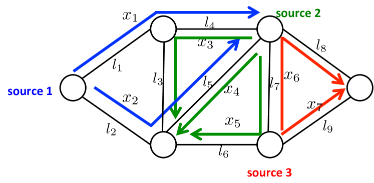
Suppose there are S𝑆S sources enumerated by 𝒮={1,2,,S}𝒮12𝑆\mathcal{S}=\{1,2,\ldots,S\} and L𝐿L links enumerated by ={1,2,,L}12𝐿\mathcal{L}=\{1,2,\ldots,L\}. Each link l𝑙l\in\mathcal{L} has a link capacity of clsubscript𝑐𝑙c_{l} bits/slot. Each source sends data from a specific origin to a specific destination, and has multiple path options. The paths for each source can use overlapping links, and they can also overlap with paths of other sources. Further, two distinct sources can have identical paths. However, it is useful to give distinct path indices to paths associated with each source (even if their corresponding paths are physically the same). Specifically, for each source s𝑠s, define 𝒫ssubscript𝒫𝑠\mathcal{P}_{s} as the set of path indices used by source s𝑠s. The index sets 𝒫1,,𝒫Ssubscript𝒫1subscript𝒫𝑆\mathcal{P}_{1},\ldots,\mathcal{P}_{S} are disjoint and 𝒫1𝒫2𝒫S=𝒦={1,2,,K}subscript𝒫1subscript𝒫2subscript𝒫𝑆𝒦12𝐾\mathcal{P}_{1}\cup\mathcal{P}_{2}\cup\cdots\cup\mathcal{P}_{S}=\mathcal{K}=\{1,2,\ldots,K\}, where K𝐾K is the number of path indices.

For each source s𝑠s, let Us(ys)subscript𝑈𝑠subscript𝑦𝑠U_{s}(y_{s}) be a real-valued, concave, continuous and nondecreasing utility function defined for ys0subscript𝑦𝑠0y_{s}\geq 0. This represents the satisfaction source s𝑠s receives by communicating with a total rate of yssubscript𝑦𝑠y_{s}, where the total rate sums over all paths it used.

Note that different paths can share links in common. Define 𝒟l𝒦subscript𝒟𝑙𝒦\mathcal{D}_{l}\subseteq\mathcal{K} as the set of paths that use link l𝑙l and ksubscript𝑘\mathcal{E}_{k}\subseteq\mathcal{L} as the set of links used by path k𝑘k. Let 𝐱=[x1,,xK]T𝐱superscriptsubscript𝑥1subscript𝑥𝐾𝑇\mathbf{x}=[x_{1},\ldots,x_{K}]^{T} be the vector that specifies the flow rate on each path; and 𝐲=[y1,,yS]T𝐲superscriptsubscript𝑦1subscript𝑦𝑆𝑇\mathbf{y}=[y_{1},\ldots,y_{S}]^{T} be the vector that specifies the rate of each source.

The goal is to allocate flow rates on each path so that no link is overloaded and network utility is maximized. This multipath network utility maximization problem can be formulated as follows:

(13) maximize s=1SUs(ys)superscriptsubscript𝑠1𝑆subscript𝑈𝑠subscript𝑦𝑠\displaystyle\sum_{s=1}^{S}U_{s}(y_{s})
(14) subject to k𝒟lxkcl,l,formulae-sequencesubscript𝑘subscript𝒟𝑙subscript𝑥𝑘subscript𝑐𝑙for-all𝑙\displaystyle\sum_{k\in\mathcal{D}_{l}}x_{k}\leq c_{l},\forall l\in\mathcal{L},
(15) ys=k𝒫sxk,s𝒮,formulae-sequencesubscript𝑦𝑠subscript𝑘subscript𝒫𝑠subscript𝑥𝑘for-all𝑠𝒮\displaystyle y_{s}=\sum_{k\in\mathcal{P}_{s}}x_{k},\forall s\in\mathcal{S},
(16) 0xkxkmax,k𝒦,formulae-sequence0subscript𝑥𝑘superscriptsubscript𝑥𝑘for-all𝑘𝒦\displaystyle 0\leq x_{k}\leq x_{k}^{\max},\forall k\in\mathcal{K},
(17) 0ysysmax,s𝒮,formulae-sequence0subscript𝑦𝑠superscriptsubscript𝑦𝑠for-all𝑠𝒮\displaystyle 0\leq y_{s}\leq y_{s}^{\max},\forall s\in\mathcal{S},

where xmaxsuperscript𝑥x^{\max} and ymaxsuperscript𝑦y^{\max} are the allowed maximum path rate and maximum source rate, respectively. The expression (13) represents the network utility; inequality (14) specifies the link capacity constraints; and equality (15) enforces the definition of yssubscript𝑦𝑠y_{s}. The linear equality constraints (15) can be formally treated by writing each one as two linear inequality constraints. However, since the utility functions Us()subscript𝑈𝑠U_{s}(\cdot) are nondecreasing and seek to maximize the yssubscript𝑦𝑠y_{s} values, it is clear that the above problem is equivalent to the following:

(18) minimize s=1SUs(ys)superscriptsubscript𝑠1𝑆subscript𝑈𝑠subscript𝑦𝑠\displaystyle-\sum_{s=1}^{S}U_{s}(y_{s})
(19) subject to k𝒟lxkcl,l,formulae-sequencesubscript𝑘subscript𝒟𝑙subscript𝑥𝑘subscript𝑐𝑙for-all𝑙\displaystyle\sum_{k\in\mathcal{D}_{l}}x_{k}\leq c_{l},\forall l\in\mathcal{L},
(20) ysk𝒫sxk,s𝒮,formulae-sequencesubscript𝑦𝑠subscript𝑘subscript𝒫𝑠subscript𝑥𝑘for-all𝑠𝒮\displaystyle y_{s}\leq\sum_{k\in\mathcal{P}_{s}}x_{k},\forall s\in\mathcal{S},
(21) 0xkxkmax,k𝒦,formulae-sequence0subscript𝑥𝑘superscriptsubscript𝑥𝑘for-all𝑘𝒦\displaystyle 0\leq x_{k}\leq x_{k}^{\max},\forall k\in\mathcal{K},
(22) 0ysysmax,s𝒮.formulae-sequence0subscript𝑦𝑠superscriptsubscript𝑦𝑠for-all𝑠𝒮\displaystyle 0\leq y_{s}\leq y_{s}^{\max},\forall s\in\mathcal{S}.

Note that the constraints (19)-(20) are linear and can be written as 𝐀[𝐱𝐲][𝐜𝟎]𝐀delimited-[]𝐱𝐲delimited-[]𝐜0\mathbf{A}\left[\begin{array}[]{c}\mathbf{x}\\ \mathbf{y}\end{array}\right]\leq\left[\begin{array}[]{c}\mathbf{c}\\ \mathbf{0}\end{array}\right], where 𝐀𝐀\mathbf{A} is an (L+S)×(K+S)𝐿𝑆𝐾𝑆(L+S)\times(K+S) matrix of which each entry is in {0,±1}0plus-or-minus1\{0,\pm 1\}. This inequality constraint 𝐀[𝐱𝐲][𝐜𝟎]𝐀delimited-[]𝐱𝐲delimited-[]𝐜0\mathbf{A}\left[\begin{array}[]{c}\mathbf{x}\\ \mathbf{y}\end{array}\right]\leq\left[\begin{array}[]{c}\mathbf{c}\\ \mathbf{0}\end{array}\right] can be treated as the inequality constraint (2) defined as 𝐠(𝐳)=𝐀𝐳𝐛𝟎𝐠𝐳𝐀𝐳𝐛0\mathbf{g}(\mathbf{z})=\mathbf{A}\mathbf{z}-\mathbf{b}\leq\mathbf{0} with 𝐳=[𝐱𝐲]𝐳delimited-[]𝐱𝐲\mathbf{z}=\left[\begin{array}[]{c}\mathbf{x}\\ \mathbf{y}\end{array}\right] and 𝐛=[𝐜𝟎]𝐛delimited-[]𝐜0\mathbf{b}=\left[\begin{array}[]{c}\mathbf{c}\\ \mathbf{0}\end{array}\right] in the general convex program (1)-(3). The box constraints (21)-(22) can be treated as the set constraint (3) in the general convex program (1)-(3). Thus, the multipath network utility maximization problem (18)-(22) is a special case of the general convex program (1)-(3).

The Lipschitz continuity of 𝐠(𝐳)𝐠𝐳\mathbf{g}(\mathbf{z}) is summarized in the next lemma.

Lemma 10.

If the constraints (19)-(20) are written as 𝐠(𝐳)𝟎𝐠𝐳0\mathbf{g}(\mathbf{z})\leq\mathbf{0}, then we have

  1. 1.

    The function 𝐠(𝐳)𝐠𝐳\mathbf{g}(\mathbf{z}) is Lipschitz continuous with modulus

    βS+K+k𝒦dk,𝛽𝑆𝐾subscript𝑘𝒦subscript𝑑𝑘\displaystyle\beta\leq\sqrt{S+K+\sum_{k\in\mathcal{K}}d_{k}},

    where dksubscript𝑑𝑘d_{k} is the length, i.e., number of hops, of path k𝒦𝑘𝒦k\in\mathcal{K}.

  2. 2.

    The function 𝐠(𝐳)𝐠𝐳\mathbf{g}(\mathbf{z}) is Lipschitz continuous with modulus β(L+1)K+S𝛽𝐿1𝐾𝑆\beta\leq\sqrt{(L+1)K+S}.

Proof.
  1. 1.

    Recall that 𝐠(𝐳)=𝐀𝐳𝐛𝐠𝐳𝐀𝐳𝐛\mathbf{g}(\mathbf{z})=\mathbf{A}\mathbf{z}-\mathbf{b} is Lipschitz continuous with modulus β=σmax(𝐀)𝛽subscript𝜎𝐀\beta=\sigma_{\max}(\mathbf{A}), where σmax(𝐀)subscript𝜎𝐀\sigma_{\max}(\mathbf{A}) is the maximum singular value of matrix 𝐀𝐀\mathbf{A}, and a simple upper bound of σmax(𝐀)subscript𝜎𝐀\sigma_{\max}(\mathbf{A}) is the Frobenius norm given by 𝐀F=tr(𝐀T𝐀)=i,jAij2subscriptnorm𝐀𝐹trsuperscript𝐀𝑇𝐀subscript𝑖𝑗superscriptsubscript𝐴𝑖𝑗2\|\mathbf{A}\|_{F}=\text{tr}(\mathbf{A}^{T}\mathbf{A})=\sqrt{\sum_{i,j}A_{ij}^{2}}. Note that 𝐀𝐀\mathbf{A} can be written as

    𝐀=[𝐑𝟎L×S𝐓𝐈S],𝐀delimited-[]𝐑subscript0𝐿𝑆𝐓subscript𝐈𝑆\displaystyle\mathbf{A}=\left[\begin{array}[]{cc}\mathbf{R}&\mathbf{0}_{L\times S}\\ -\mathbf{T}&\mathbf{I}_{S}\end{array}\right],

    where 𝐑𝐑\mathbf{R} is a {0,1}01\{0,1\} matrix of size L×K𝐿𝐾L\times K , 𝟎L×Ssubscript0𝐿𝑆\mathbf{0}_{L\times S} is an L×S𝐿𝑆L\times S zero matrix, 𝐓𝐓\mathbf{T} is a {0,1}01\{0,1\} matrix of size S×K𝑆𝐾S\times K and 𝐈Ssubscript𝐈𝑆\mathbf{I}_{S} is an S×S𝑆𝑆S\times S identity matrix. Note that the (l,k)𝑙𝑘(l,k)-th entry of 𝐑𝐑\mathbf{R} is 111 if and only if path k𝑘k uses link l𝑙l; the (s,k)𝑠𝑘(s,k)-th entry of 𝐓𝐓\mathbf{T} is 111 if and only if path k𝑘k is a path for source s𝑠s, i.e, k𝒫s𝑘subscript𝒫𝑠k\in\mathcal{P}_{s}. Matrix 𝐑𝐑\mathbf{R} has k𝒦dksubscript𝑘𝒦subscript𝑑𝑘\sum_{k\in\mathcal{K}}d_{k} non-zero entries since each column has exactly dksubscript𝑑𝑘d_{k} non-zero entries. Matrix 𝐓𝐓\mathbf{T} has K𝐾K non-zero entries since there are in total K𝐾K network paths. Thus, matrix 𝐀𝐀\mathbf{A} in total has S+K+k𝒦dk𝑆𝐾subscript𝑘𝒦subscript𝑑𝑘S+K+\sum_{k\in\mathcal{K}}d_{k} non-zero entries whose absolute values are equal to 111. It follows that βS+K+k𝒦dk𝛽𝑆𝐾subscript𝑘𝒦subscript𝑑𝑘\beta\leq\sqrt{S+K+\sum_{k\in\mathcal{K}}d_{k}}.

  2. 2.

    This part follows from the fact that the length of each path is at most L𝐿L.

Note that the second bound in the above lemma is more loose than the first one but holds regardless of the flow path configurations in the network. A straightforward application of Algorithm 1 yields the following decentralized network flow control algorithm described in Algorithm 2. Similar to the flow control based on the dual subgradient algorithm, Algorithm 2 is decentralized and can be easily implemented within the current TCP protocols [10].

Algorithm 2
  • Initialization: Let xk(1)[0,xkmax],ksubscript𝑥𝑘10superscriptsubscript𝑥𝑘for-all𝑘x_{k}(-1)\in[0,x_{k}^{\max}],\forall k be arbitrary, ys(1)[0,ysmax],ssubscript𝑦𝑠10superscriptsubscript𝑦𝑠for-all𝑠y_{s}(-1)\in[0,y_{s}^{\max}],\forall s be arbitrary, Ql(0)=max{0,k𝒟lxk(1)+cl},lformulae-sequencesubscript𝑄𝑙00subscript𝑘subscript𝒟𝑙subscript𝑥𝑘1subscript𝑐𝑙for-all𝑙Q_{l}(0)=\max\{0,-\sum_{k\in\mathcal{D}_{l}}x_{k}(-1)+c_{l}\},\forall l\in\mathcal{L}, Yl(0)=Ql(0)+k𝒟lxk(1)cl,lformulae-sequencesubscript𝑌𝑙0subscript𝑄𝑙0subscript𝑘subscript𝒟𝑙subscript𝑥𝑘1subscript𝑐𝑙for-all𝑙Y_{l}(0)=Q_{l}(0)+\sum_{k\in\mathcal{D}_{l}}x_{k}(-1)-c_{l},\forall l\in\mathcal{L}, Rs(0)=max{0,k𝒫sxk(1)ys(1)},s𝒮formulae-sequencesubscript𝑅𝑠00subscript𝑘subscript𝒫𝑠subscript𝑥𝑘1subscript𝑦𝑠1for-all𝑠𝒮R_{s}(0)=\max\{0,\sum_{k\in\mathcal{P}_{s}}x_{k}(-1)-y_{s}(-1)\},\forall s\in\mathcal{S} and Zs(0)=Rs(0)+ys(1)k𝒫sxk(1),s𝒮formulae-sequencesubscript𝑍𝑠0subscript𝑅𝑠0subscript𝑦𝑠1subscript𝑘subscript𝒫𝑠subscript𝑥𝑘1for-all𝑠𝒮Z_{s}(0)=R_{s}(0)+y_{s}(-1)-\sum_{k\in\mathcal{P}_{s}}x_{k}(-1),\forall s\in\mathcal{S}.

  • Each link l𝑙l’s algorithm: At each time t{0,1,}𝑡01t\in\{0,1,\ldots\}, link l𝑙l does the following:

    1. 1.

      Receive the path rates xk(t)subscript𝑥𝑘𝑡x_{k}(t) that use link l𝑙l. Update Ql(t)subscript𝑄𝑙𝑡Q_{l}(t) via:

      Ql(t+1)=max{k𝒟lxk(t)+cl,Ql(t)+k𝒟lxk(t)cl}.subscript𝑄𝑙𝑡1subscript𝑘subscript𝒟𝑙subscript𝑥𝑘𝑡subscript𝑐𝑙subscript𝑄𝑙𝑡subscript𝑘subscript𝒟𝑙subscript𝑥𝑘𝑡subscript𝑐𝑙\displaystyle Q_{l}(t+1)=\max\Big{\{}-\sum_{k\in\mathcal{D}_{l}}x_{k}(t)+c_{l},Q_{l}(t)+\sum_{k\in\mathcal{D}_{l}}x_{k}(t)-c_{l}\Big{\}}.
    2. 2.

      The price of this link is given by Yl(t+1)=Ql(t+1)+k𝒟lxk(t)clsubscript𝑌𝑙𝑡1subscript𝑄𝑙𝑡1subscript𝑘subscript𝒟𝑙subscript𝑥𝑘𝑡subscript𝑐𝑙Y_{l}(t+1)=Q_{l}(t+1)+\sum_{k\in\mathcal{D}_{l}}x_{k}(t)-c_{l}.

    3. 3.

      Communicate the link price Yl(t+1)subscript𝑌𝑙𝑡1Y_{l}(t+1) to sources that use link l𝑙l.

  • Each source s𝑠s’s algorithm: At each time t{0,1,}𝑡01t\in\{0,1,\ldots\}, source s𝑠s does the following:

    1. 1.

      Receive from the network the link prices Yl(t)subscript𝑌𝑙𝑡Y_{l}(t) for all links l𝑙l that are used by any path of source s𝑠s.

    2. 2.

      Update the path rates xk,k𝒫ssubscript𝑥𝑘𝑘subscript𝒫𝑠x_{k},k\in\mathcal{P}_{s} by

      xk(t)subscript𝑥𝑘𝑡\displaystyle x_{k}(t) =argmin0xkxkmax{[lkYl(t)Zs(t)]xk+α(xkxk(t1))2}absentsubscriptargmin0subscript𝑥𝑘superscriptsubscript𝑥𝑘delimited-[]subscript𝑙subscript𝑘subscript𝑌𝑙𝑡subscript𝑍𝑠𝑡subscript𝑥𝑘𝛼superscriptsubscript𝑥𝑘subscript𝑥𝑘𝑡12\displaystyle=\operatorname*{argmin}_{0\leq x_{k}\leq x_{k}^{\max}}\Big{\{}\big{[}\sum_{l\in\mathcal{E}_{k}}Y_{l}(t)-Z_{s}(t)\big{]}x_{k}+\alpha(x_{k}-x_{k}(t-1))^{2}\Big{\}}
      =[xk(t1)12α(lkYl(t)Zs(t))]0xkmax,absentsuperscriptsubscriptdelimited-[]subscript𝑥𝑘𝑡112𝛼subscript𝑙subscript𝑘subscript𝑌𝑙𝑡subscript𝑍𝑠𝑡0superscriptsubscript𝑥𝑘\displaystyle=\Big{[}x_{k}(t-1)-\frac{1}{2\alpha}\big{(}\sum_{l\in\mathcal{E}_{k}}Y_{l}(t)-Z_{s}(t)\big{)}\Big{]}_{0}^{x_{k}^{\max}},

      where [z]ab=min{max{z,a},b}subscriptsuperscriptdelimited-[]𝑧𝑏𝑎𝑧𝑎𝑏[z]^{b}_{a}=\min\{\max\{z,a\},b\}.

    3. 3.

      Communicate the path rates xk(t),k𝒫ssubscript𝑥𝑘𝑡𝑘subscript𝒫𝑠x_{k}(t),k\in\mathcal{P}_{s} to all links that are used by path k𝑘k.

    4. 4.

      Update the source rate ys(t)subscript𝑦𝑠𝑡y_{s}(t) by

      ys(t)=argmin0ysysmax{Us(ys)+Zs(t)ys+α(ysys(t1))2},subscript𝑦𝑠𝑡subscriptargmin0subscript𝑦𝑠superscriptsubscript𝑦𝑠subscript𝑈𝑠subscript𝑦𝑠subscript𝑍𝑠𝑡subscript𝑦𝑠𝛼superscriptsubscript𝑦𝑠subscript𝑦𝑠𝑡12\displaystyle y_{s}(t)=\operatorname*{argmin}_{0\leq y_{s}\leq y_{s}^{\max}}\Big{\{}-U_{s}(y_{s})+Z_{s}(t)y_{s}+\alpha(y_{s}-y_{s}(t-1))^{2}\Big{\}},

      which usually has a closed form solution for differentiable utilities by taking derivatives.

    5. 5.

      Update virtual queue Rs(t)subscript𝑅𝑠𝑡R_{s}(t) and source price Zs(t)subscript𝑍𝑠𝑡Z_{s}(t) locally by

      Rs(t+1)subscript𝑅𝑠𝑡1\displaystyle R_{s}(t+1) =max{ys(t)+k𝒫sxk(t),Rs(t)+ys(t)k𝒫sxk(t)},absentsubscript𝑦𝑠𝑡subscript𝑘subscript𝒫𝑠subscript𝑥𝑘𝑡subscript𝑅𝑠𝑡subscript𝑦𝑠𝑡subscript𝑘subscript𝒫𝑠subscript𝑥𝑘𝑡\displaystyle=\max\Big{\{}-y_{s}(t)+\sum_{k\in\mathcal{P}_{s}}x_{k}(t),R_{s}(t)+y_{s}(t)-\sum_{k\in\mathcal{P}_{s}}x_{k}(t)\Big{\}},
      Zs(t+1)subscript𝑍𝑠𝑡1\displaystyle Z_{s}(t+1) =Rs(t+1)+ys(t)k𝒫sxk(t).absentsubscript𝑅𝑠𝑡1subscript𝑦𝑠𝑡subscript𝑘subscript𝒫𝑠subscript𝑥𝑘𝑡\displaystyle=R_{s}(t+1)+y_{s}(t)-\sum_{k\in\mathcal{P}_{s}}x_{k}(t).

By 3, if we choose α12(S+K+k𝒦dk)𝛼12𝑆𝐾subscript𝑘𝒦subscript𝑑𝑘\alpha\geq\frac{1}{2}\big{(}S+K+\sum_{k\in\mathcal{K}}d_{k}\big{)}, then for any t1𝑡1t\geq 1,

(23) s=1SUs(y¯s(t))superscriptsubscript𝑠1𝑆subscript𝑈𝑠subscript¯𝑦𝑠𝑡\displaystyle\sum_{s=1}^{S}U_{s}(\overline{y}_{s}(t)) s=1SUs(ys)O(1/t),absentsuperscriptsubscript𝑠1𝑆subscript𝑈𝑠superscriptsubscript𝑦𝑠𝑂1𝑡\displaystyle\geq\sum_{s=1}^{S}U_{s}(y_{s}^{\ast})-O(1/t),
(24) k𝒟lx¯k(t)subscript𝑘subscript𝒟𝑙subscript¯𝑥𝑘𝑡\displaystyle\sum_{k\in\mathcal{D}_{l}}\overline{x}_{k}(t) cl+O(1/t),l,formulae-sequenceabsentsubscript𝑐𝑙𝑂1𝑡for-all𝑙\displaystyle\leq c_{l}+O(1/t),\qquad\qquad\quad~{}~{}\forall l\in\mathcal{L},
(25) y¯s(t)subscript¯𝑦𝑠𝑡\displaystyle\overline{y}_{s}(t) k𝒫sx¯k(t)+O(1/t),s𝒮,formulae-sequenceabsentsubscript𝑘subscript𝒫𝑠subscript¯𝑥𝑘𝑡𝑂1𝑡for-all𝑠𝒮\displaystyle\leq\sum_{k\in\mathcal{P}_{s}}\overline{x}_{k}(t)+O(1/t),\qquad\forall s\in\mathcal{S},

where (𝐱,𝐲)superscript𝐱superscript𝐲(\mathbf{x}^{\ast},\mathbf{y}^{\ast}) is an optimal solution of the problem (18)-(22). Note that if Algorithm 2 has been run for a sufficiently long time and we are satisfied with the current performance, then we can fix 𝐱=1tτ=0t1𝐱(τ)𝐱1𝑡superscriptsubscript𝜏0𝑡1𝐱𝜏\mathbf{x}=\frac{1}{t}\sum_{\tau=0}^{t-1}\mathbf{x}(\tau) and 𝐲=1tτ=0t1𝐲(τ)𝐲1𝑡superscriptsubscript𝜏0𝑡1𝐲𝜏\mathbf{y}=\frac{1}{t}\sum_{\tau=0}^{t-1}\mathbf{y}(\tau) such that the performance is still within O(1/t)𝑂1𝑡O(1/t) sub-optimality for all future time.

4.3 Decentralized Joint Flow and Power Control

Since Algorithm 1 allows for general nonlinear convex constraint functions, it can also be applied to solve the joint flow and power control problem. In this case, the capacity of each link l𝑙l is not fixed but depends concavely on a power allocation variable plsubscript𝑝𝑙p_{l}. Assuming each link capacity is logarithmic in plsubscript𝑝𝑙p_{l} results in the following problem:

(26) maximize s=1SUs(ys)l=1LVl(pl)superscriptsubscript𝑠1𝑆subscript𝑈𝑠subscript𝑦𝑠superscriptsubscript𝑙1𝐿subscript𝑉𝑙subscript𝑝𝑙\displaystyle\sum_{s=1}^{S}U_{s}(y_{s})-\sum_{l=1}^{L}V_{l}(p_{l})
(27) subject to k𝒟lxklog(1+pl),l,formulae-sequencesubscript𝑘subscript𝒟𝑙subscript𝑥𝑘1subscript𝑝𝑙for-all𝑙\displaystyle\sum_{k\in\mathcal{D}_{l}}x_{k}\leq\log(1+p_{l}),\forall l\in\mathcal{L},
(28) ysk𝒫sxk,s𝒮,formulae-sequencesubscript𝑦𝑠subscript𝑘subscript𝒫𝑠subscript𝑥𝑘for-all𝑠𝒮\displaystyle y_{s}\leq\sum_{k\in\mathcal{P}_{s}}x_{k},\forall s\in\mathcal{S},
(29) 0xkxkmax,k𝒦,formulae-sequence0subscript𝑥𝑘superscriptsubscript𝑥𝑘for-all𝑘𝒦\displaystyle 0\leq x_{k}\leq x_{k}^{\max},\forall k\in\mathcal{K},
(30) 0ysysmax,s𝒮,formulae-sequence0subscript𝑦𝑠superscriptsubscript𝑦𝑠for-all𝑠𝒮\displaystyle 0\leq y_{s}\leq y_{s}^{\max},\forall s\in\mathcal{S},
(31) 0plplmax,l,formulae-sequence0subscript𝑝𝑙superscriptsubscript𝑝𝑙for-all𝑙\displaystyle 0\leq p_{l}\leq p_{l}^{\max},\forall l\in\mathcal{L},

where plsubscript𝑝𝑙p_{l} is the power allocated at link l𝑙l, log(1+pl)1subscript𝑝𝑙\log(1+p_{l}) is the corresponding link capacity as a function of plsubscript𝑝𝑙p_{l}, and Vl(pl)subscript𝑉𝑙subscript𝑝𝑙V_{l}(p_{l}) is the associated power cost (assumed to be a convex function of plsubscript𝑝𝑙p_{l}). A decentralized joint flow and power control algorithm for this problem can be similarly developed by applying Algorithm 1.

5 Numerical Results

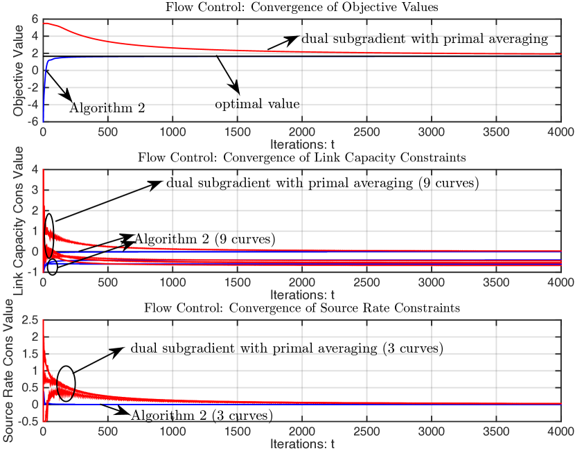
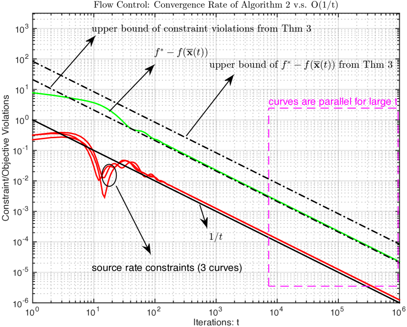
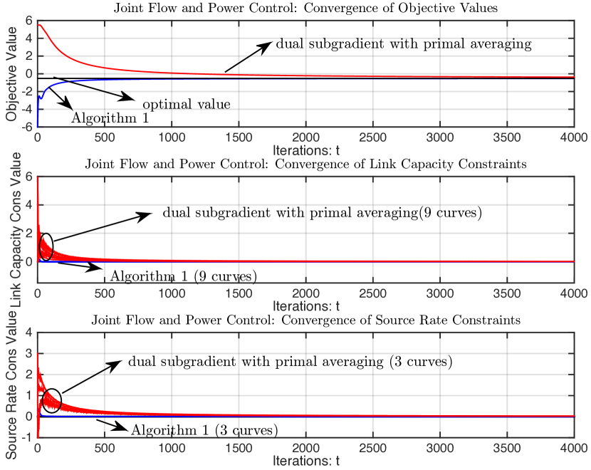
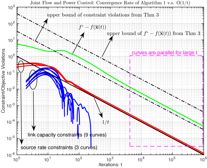
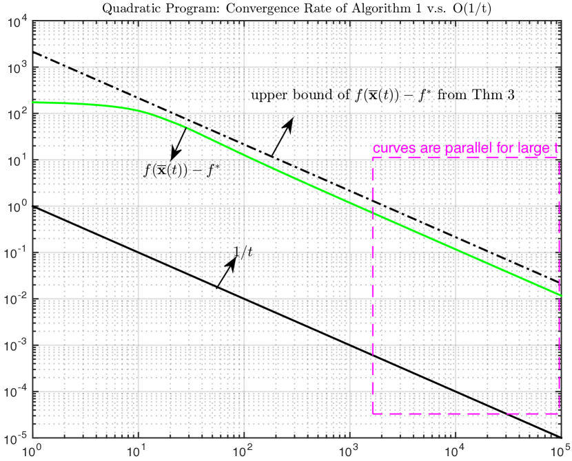
This section considers numerical experiments to verify the convergence rate results shown in this paper.

5.1 Decentralized Multiplath Flow Control

Consider the simple multipath network flow problem described in Fig. 1. Assume each link has capacity 111. Let y1,y2subscript𝑦1subscript𝑦2y_{1},y_{2} and y3subscript𝑦3y_{3} be the data rates of source 1,2121,2 and 333; x1,x2,x3,x4,x5,x6subscript𝑥1subscript𝑥2subscript𝑥3subscript𝑥4subscript𝑥5subscript𝑥6x_{1},x_{2},x_{3},x_{4},x_{5},x_{6} and x7subscript𝑥7x_{7} be the data rates of the paths indicated in the figure; and the network utility be maximizing log(y1)+2log(y2)+2log(y3)subscript𝑦12subscript𝑦22subscript𝑦3\log(y_{1})+2\log(y_{2})+2\log(y_{3}). The NUM problem can be formulated as follows:

maximize log(y1)+2log(y2)+2log(y3)subscript𝑦12subscript𝑦22subscript𝑦3\displaystyle\log(y_{1})+2\log(y_{2})+2\log(y_{3})
subject to 𝐑𝐱𝐜,𝐑𝐱𝐜\displaystyle\mathbf{R}\mathbf{x}\leq\mathbf{c},
𝐲𝐓𝐱,𝐲𝐓𝐱\displaystyle\mathbf{y}\leq\mathbf{T}\mathbf{x},
0xiximax,i{1,2,,4},formulae-sequence0subscript𝑥𝑖superscriptsubscript𝑥𝑖𝑖124\displaystyle 0\leq x_{i}\leq x_{i}^{\max},i\in\{1,2,\ldots,4\},
0yiyimax,i{1,2,3},formulae-sequence0subscript𝑦𝑖superscriptsubscript𝑦𝑖𝑖123\displaystyle 0\leq y_{i}\leq y_{i}^{\max},i\in\{1,2,3\},

where 𝐑=[100000001000000010000101000001010000000100000011000000100000001],𝐜=[111111111]formulae-sequence𝐑delimited-[]100000001000000010000101000001010000000100000011000000100000001𝐜delimited-[]111111111\mathbf{R}=\left[\begin{array}[]{ccccccc}1&0&0&0&0&0&0\\ 0&1&0&0&0&0&0\\ 0&0&1&0&0&0&0\\ 1&0&1&0&0&0&0\\ 0&1&0&1&0&0&0\\ 0&0&0&0&1&0&0\\ 0&0&0&0&1&1&0\\ 0&0&0&0&0&1&0\\ 0&0&0&0&0&0&1\end{array}\right],\mathbf{c}=\left[\begin{array}[]{c}1\\ 1\\ 1\\ 1\\ 1\\ 1\\ 1\\ 1\\ 1\end{array}\right], 𝐓=[110000000111000000011]𝐓delimited-[]110000000111000000011\mathbf{T}=\left[\begin{array}[]{ccccccc}1&1&0&0&0&0&0\\ 0&0&1&1&1&0&0\\ 0&0&0&0&0&1&1\end{array}\right]. The optimal value to this NUM problem is f=1.65687superscript𝑓1.65687f^{\ast}=1.65687.

To verify the convergence of Algorithm 2, Fig. 2 shows the values of objective and constraint functions yielded by Algorithm 2 with α=12(K+S+k𝒦dk)+1=10𝛼12𝐾𝑆subscript𝑘𝒦subscript𝑑𝑘110\alpha=\frac{1}{2}\big{(}K+S+\sum_{k\in\mathcal{K}}d_{k}\big{)}+1=10 and 𝐱(1)=𝟎𝐱10\mathbf{x}(-1)=\mathbf{0}. (By writing constraints 𝐑𝐱𝐜𝐑𝐱𝐜\mathbf{R}\mathbf{x}\leq\mathbf{c} and 𝐲𝐓𝐱𝐲𝐓𝐱\mathbf{y}\leq\mathbf{T}\mathbf{x} in the compact form 𝐀𝐳𝐛𝐀𝐳𝐛\mathbf{A}\mathbf{z}\leq\mathbf{b}, it can be checked that β=σmax(𝐀)=2.4307𝛽subscript𝜎𝐀2.4307\beta=\sigma_{\max}(\mathbf{A})=2.4307. If we choose a smaller α𝛼\alpha, e.g., α=12β2+1=3.9543𝛼12superscript𝛽213.9543\alpha=\frac{1}{2}\beta^{2}+1=3.9543, then Algorithm 2 converges even faster. In this simulation, we choose a loose α𝛼\alpha whose value can be easily estimated from 10 without knowing the detailed network topology.) We also compare our algorithm with the dual subgradient algorithm (with primal averaging) with step size 0.010.010.01 in [13]. (Or equivalently, the DPP algorithm with V=100𝑉100V=100 in [15, 17, 23].) Recall that the dual subgradient algorithm in [15, 13, 17, 23] does not converge to an exact optimal solution but only converges to an approximate solution with an error level determined by the step size. In contrast, our algorithm can eventually converge to the exact optimality. Fig. 2 shows that Algorithm 2 converges faster than the dual subgradient algorithm with primal averaging.

To verify the convergence rate of Algorithm 2, Fig. 3 plots f(𝐱¯(t))f𝑓¯𝐱𝑡superscript𝑓f(\overline{\mathbf{x}}(t))-f^{\ast}, all constraint values, function 1/t1𝑡1/t, and bounds from 3 with both x-axis and y-axis in log10subscript10\log_{10} scales. It can be observed that the curves of f(𝐱¯(t))f𝑓¯𝐱𝑡superscript𝑓f(\overline{\mathbf{x}}(t))-f^{\ast} and all the source rate constraint values are parallel to the curve of 1/t1𝑡1/t for large t𝑡t. Note that all the link capacity constraints are satisfied early (i.e., negative), and hence are not drawn in log10subscript10\log_{10} scales. Fig. 3 verifies that the error of Algorithm 2 decays like O(1/t)𝑂1𝑡O(1/t) and suggests that it is actually Θ(1/t)Θ1𝑡\Theta(1/t) for this multipath NUM problem.

Refer to caption
Figure 1: A simple multipath NUM problem with 333 sources and 777 paths.
Refer to caption
Figure 2: The convergence of Algorithm 2 and the dual subgradient algorithm with primal averaging for a multipath flow control problem.
Refer to caption
Figure 3: The convergence rate of Algorithm 2 for a multipath flow control problem.

5.2 Decentralized Joint Flow and Power Control

Consider the joint flow and power control over the same network described in Fig. 1. We assume the power cost of each link is given by Vl(pl)=0.25plsubscript𝑉𝑙subscript𝑝𝑙0.25subscript𝑝𝑙V_{l}(p_{l})=0.25p_{l}. The optimal value of this joint flow and power control problem is f=0.521318superscript𝑓0.521318f^{\ast}=-0.521318.

To verify the convergence of Algorithm 1, Fig. 4 shows the values of objective and constraint functions yielded by Algorithm 1 with α=10𝛼10\alpha=10, 𝐱(1)=𝟎𝐱10\mathbf{x}(-1)=\mathbf{0}, 𝐲(1)=𝟎𝐲10\mathbf{y}(-1)=\mathbf{0} and 𝐩(1)=𝟎𝐩10\mathbf{p}(-1)=\mathbf{0}. (In fact, by writing constraints 𝐑𝐱log(1+𝐩)𝐑𝐱1𝐩\mathbf{R}\mathbf{x}\leq\log(1+\mathbf{p}) and 𝐲𝐓𝐱𝐲𝐓𝐱\mathbf{y}\leq\mathbf{T}\mathbf{x} in the compact form 𝐠(𝐳)𝟎𝐠𝐳0\mathbf{g}(\mathbf{z})\leq\mathbf{0}, it can be checked that β=2.5229𝛽2.5229\beta=2.5229. If we choose a smaller α𝛼\alpha, e.g., α=12β2+1=4.1826𝛼12superscript𝛽214.1826\alpha=\frac{1}{2}\beta^{2}+1=4.1826, then Algorithm 1 converges even faster.) We also compare our algorithm with the dual subgradient algorithm (with primal averaging) with step size 0.010.010.01 in [15, 13, 17, 23]. Fig. 4 shows that Algorithm 1 converges faster than the dual subgradient algorithm with primal averaging.

To verify the convergence rate of Algorithm 1, Fig. 5 plots f(𝐱¯(t))f𝑓¯𝐱𝑡superscript𝑓f(\overline{\mathbf{x}}(t))-f^{\ast}, all constraint values, function 1/t1𝑡1/t, and bounds from 3 with both x-axis and y-axis in log10subscript10\log_{10} scales. It can be observed that the curves of f(𝐱¯(t))f𝑓¯𝐱𝑡superscript𝑓f(\overline{\mathbf{x}}(t))-f^{\ast} and all the source rate constraint values are parallel to the curve of 1/t1𝑡1/t for large t𝑡t.

Refer to caption
Figure 4: The convergence of Algorithm 1 and the dual subgradient algorithm with primal averaging for a multipath joint flow and power control problem.
Refer to caption
Figure 5: The convergence rate of Algorithm 1 for a multipath joint flow and power control problem.

5.3 Quadratic Programs

Consider the following quadratic program

min\displaystyle\min~{}~{} 𝐱T𝐏𝐱+𝐜T𝐱superscript𝐱𝑇𝐏𝐱superscript𝐜𝑇𝐱\displaystyle\mathbf{x}^{T}\mathbf{P}\mathbf{x}+\mathbf{c}^{T}\mathbf{x}
s.t. 𝐱T𝐐𝐱+𝐝T𝐱esuperscript𝐱𝑇𝐐𝐱superscript𝐝𝑇𝐱𝑒\displaystyle\mathbf{x}^{T}\mathbf{Q}\mathbf{x}+\mathbf{d}^{T}\mathbf{x}\leq e
𝐱min𝐱𝐱maxsuperscript𝐱𝐱superscript𝐱\displaystyle\mathbf{x}^{\min}\leq\mathbf{x}\leq\mathbf{x}^{\max}

where 𝐏𝐏\mathbf{P} and 𝐐𝐐\mathbf{Q} are positive semidefinite to ensure the convexity of the quadratic program.

We randomly generate a large scale example where 𝐱100𝐱superscript100\mathbf{x}\in\mathbb{R}^{100}, 𝐏100×100𝐏superscript100100\mathbf{P}\in\mathbb{R}^{100\times 100} is diagonal with entries from uniform [0,4]04[0,4], 𝐜100𝐜superscript100\mathbf{c}\in\mathbb{R}^{100} with entries from uniform [15,20]1520[-15,20], 𝐐100×100𝐐superscript100100\mathbf{Q}\in\mathbb{R}^{100\times 100} is diagonal with entries from uniform [0,1]01[0,1], 𝐝100𝐝superscript100\mathbf{d}\in\mathbb{R}^{100} with entries from uniform [1,1]11[-1,1], e𝑒e is a scalar from uniform [4,5]45[4,5], 𝐱min=𝟎superscript𝐱0\mathbf{x}^{\min}=\mathbf{0} and 𝐱max=𝟏superscript𝐱1\mathbf{x}^{\max}=\mathbf{1}. Note that Algorithm 1 and the dual subgradient algorithm (with primal averaging) can deal with general semidefinite positive matrices 𝐏𝐏\mathbf{P} and 𝐐𝐐\mathbf{Q}. However, if 𝐏𝐏\mathbf{P} and 𝐐𝐐\mathbf{Q} are diagonal or block diagonal, then the primal update in both algorithms can be decomposed into independent smaller problems and hence has extremely low complexity.

To verify the convergence of Algorithm 1, Fig. 6 shows the values of objective and constraint functions yielded by Algorithm 1 with α=12β2+1𝛼12superscript𝛽21\alpha=\frac{1}{2}\beta^{2}+1, where β𝛽\beta the is Lipschitz modulus of the constraint function, and 𝐱(1)=𝐱min𝐱1superscript𝐱\mathbf{x}(-1)=\mathbf{x}^{\min}. We also compare our algorithm with the dual subgradient algorithm (with primal averaging) with step size 0.010.010.01 in [15, 13, 17, 23]. Fig. 6 shows that Algorithm 1 converges faster than the dual subgradient algorithm with primal averaging.

To verify the convergence rate of Algorithm 1, Fig. 7 plots f(𝐱¯(t))f𝑓¯𝐱𝑡superscript𝑓f(\overline{\mathbf{x}}(t))-f^{\ast}, function 1/t1𝑡1/t, and the bound from 3 with both x-axis and y-axis in log10subscript10\log_{10} scales. It can be observed that the curves of f(𝐱¯(t))f𝑓¯𝐱𝑡superscript𝑓f(\overline{\mathbf{x}}(t))-f^{\ast} and all the source rate constraint values are parallel to the curve of 1/t1𝑡1/t for large t𝑡t. Note that the constraint violation is not plotted since the constraint function is satisfied for all iterations as observed in Fig. 6.
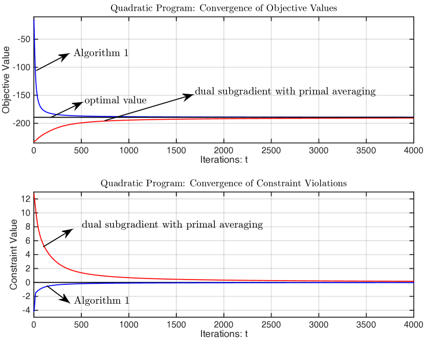
Refer to caption
Figure 6: The convergence of Algorithm 1 and the dual subgradient algorithm with primal averaging for a quadratic program.
Refer to caption
Figure 7: The convergence rate of Algorithm 1 for a quadratic program.

6 Conclusions

This paper proposes a novel but simple algorithm to solve convex programs with a possibly non-differentiable objective function and Lipschitz continuous constraint functions. The new algorithm has a parallel implementation when the objective function and constraint functions are separable. The convergence rate of the proposed algorithm is shown to be O(1/t)𝑂1𝑡O(1/t). This is faster than the O(1/t)𝑂1𝑡O(1/\sqrt{t}) convergence rate of the dual subgradient algorithm with primal averaging. The ADMM algorithm has the same O(1/t)𝑂1𝑡O(1/t) convergence rate but can only deal with linear equality constraint functions. The new algorithm is further applied to solve multipath network flow control problems and yields a decentralized flow control algorithm which converges faster than existing dual subgradient or primal-dual subgradient based flow control algorithms. The O(1/t)𝑂1𝑡O(1/t) convergence rate of the proposed algorithm is also verified by numerical experiments.

References

  • [1] M. S. Bazaraa, H. D. Sherali, and C. M. Shetty, Nonlinear Programming: Theory and Algorithms, Wiley-Interscience, 2006.
  • [2] A. Beck, A. Nedic, A. Ozdaglar, and M. Teboulle, An O(1/k)𝑂1𝑘{O}(1/k) gradient method for network resource allocation problems, IEEE Transactions on Control of Network Systems, 1 (2014), pp. 64–73.
  • [3] D. P. Bertsekas, Nonlinear Programming, Athena Scientific, second ed., 1999.
  • [4] S. Boyd, N. Parikh, E. Chu, B. Peleato, and J. Eckstein, Distributed optimization and statistical learning via the alternating direction method of multipliers, Foundations and Trends in Machine Learning, 3 (2011), pp. 1–122.
  • [5] S. Boyd and L. Vandenberghe, Convex Optimization, Cambridge University Press, 2004.
  • [6] B. He and X. Yuan, On the O(1/n)𝑂1𝑛{O}(1/n) convergence rate of the Douglas-Rachford alternating direction method, SIAM Journal on Numerical Analysis, 50 (2012), pp. 700–709.
  • [7] J.-B. Hiriart-Urruty and C. Lemaréchal, Fundamentals of Convex Analysis, Springer, 2001.
  • [8] F. P. Kelly, A. K. Maulloo, and D. K. Tan, Rate control for communication networks: Shadow prices, proportional fairness and stability, Journal of the Operational Research Society, (1998), pp. 237–252.
  • [9] T.-Y. Lin, S.-Q. Ma, and S.-Z. Zhang, On the sublinear convergence rate of multi-block ADMM, Journal of the Operations Research Society of China, 3 (2015), pp. 251–274.
  • [10] S. H. Low, A duality model of TCP flow controls, in Proceedings of ITC Specialist Seminar on IP Traffic Measurement, Modeling and Management, 2000.
  • [11] S. H. Low and D. E. Lapsley, Optimization flow control—I: basic algorithm and convergence, IEEE/ACM Transactions on Networking, 7 (1999), pp. 861–874.
  • [12] I. Necoara and V. Nedelcu, Rate analysis of inexact dual first-order methods application to dual decomposition, IEEE Transactions on Automatic Control, 59 (2014), pp. 1232–1243.
  • [13] A. Nedić and A. Ozdaglar, Approximate primal solutions and rate analysis for dual subgradient methods, SIAM Journal on Optimization, 19 (2009), pp. 1757–1780.
  • [14] A. Nedić and A. Ozdaglar, Subgradient methods for saddle-point problems, Journal of Optimization Theory and Applications, 142 (2009), pp. 205–228.
  • [15] M. J. Neely, Distributed and secure computation of convex programs over a network of connected processors, in DCDIS Conference Guelph, 2005.
  • [16] M. J. Neely, Stochastic Network Optimization with Application to Communication and Queueing Systems, Morgan & Claypool Publishers, 2010.
  • [17] M. J. Neely, A simple convergence time analysis of drift-plus-penalty for stochastic optimization and convex programs, arXiv:1412.0791, (2014).
  • [18] Y. Nesterov, Introductory Lectures on Convex Optimization: A Basic Course, Springer Science & Business Media, 2004.
  • [19] N. Parikh and S. Boyd, Proximal algorithms, Foundations and Trends in Optimization, 1 (2013), pp. 123–231.
  • [20] W.-H. Wang, M. Palaniswami, and S. H. Low, Optimal flow control and routing in multi-path networks, Performance Evaluation, 52 (2003), pp. 119–132.
  • [21] E. Wei and A. Ozdaglar, On the O(1/k)𝑂1𝑘{O}(1/k) convergence of asynchronous distributed alternating direction method of multipliers, in Proc. IEEE Global Conference on Signal and Information Processing, 2013.
  • [22] E. Wei, A. Ozdaglar, and A. Jadbabaie, A distributed Newton method for network utility maximization–I: algorithm, IEEE Transactions on Automatic Control, 58 (2013), pp. 2162–2175.
  • [23] H. Yu and M. J. Neely, On the convergence time of the drift-plus-penalty algorithm for strongly convex programs, in Proceedings of IEEE Conference on Decision and Control (CDC), 2015.
  • [24] H. Yu and M. J. Neely, A primal-dual type algorithm with the O(1/t)𝑂1𝑡{O}(1/t) convergence rate for large scale constrained convex programs, in Proceedings of IEEE Conference on Decision and Control (CDC), 2016.