Hook formulas for skew shapes I. $q$-analogues and bijections

Abstract.

The celebrated hook-length formula gives a product formula for the number of standard Young tableaux of a straight shape. In 2014, Naruse announced a more general formula for the number of standard Young tableaux of skew shapes as a positive sum over excited diagrams of products of hook-lengths. We give an algebraic and a combinatorial proof of Naruse’s formula, by using factorial Schur functions and a generalization of the Hillman–Grassl correspondence, respectively.

The main new results are two different $q$-analogues of Naruse’s formula: for the skew Schur functions, and for counting reverse plane partitions of skew shapes. We establish explicit bijections between these objects and families of integer arrays with certain nonzero entries, which also proves the second formula.

smalltableaux

1. Introduction

1.1. Foreword

The classical hook-length formula (HLF) for the number of standard Young tableaux (SYT) of a Young diagram, is a beautiful result in enumerative combinatorics that is both mysterious and extremely well studied. In a way it is a perfect formula – highly nontrivial, clean, concise and generalizing several others (binomial coefficients, Catalan numbers, etc.) The HLF was discovered by Frame, Robinson and Thrall [FRT] in 1954, and by now it has numerous proofs: probabilistic, bijective, inductive, analytic, geometric, etc. (see $\S$10.3). Arguably, each of these proofs does not really explain the HLF on a deeper level, but rather tells a different story, leading to new generalizations and interesting connections to other areas. In this paper we prove a new generalization of the HLF for skew shapes which presented an unusual and interesting challenge; it has yet to be fully explained and understood.

For skew shapes, there is no product formula for the number $f^{\lambda/\mu}$ of standard Young tableaux (cf. Section 9). Most recently, in the context of equivariant Schubert calculus, Naruse presented and outlined a proof in [Naru] of a remarkable generalization on the HLF, which we call the Naruse hook-length formula (NHLF). This formula (see below), writes $f^{\lambda/\mu}$ as a sum of “hook products” over the excited diagrams, defined as certain generalizations of skew shapes. These excited diagrams were introduced by Ikeda and Naruse [IN1], and in a slightly different form independently by Kreiman [Kre1, Kre2] and Knutson, Miller and Yong [KMY]. They are a combinatorial model for the terms appearing in the formula for Kostant polynomials discovered independently by Andersen, Jantzen and Soergel [AJS, Appendix D], and Billey [Bil] (see Remark 4.2 and $\S$10.4). These diagrams are the main combinatorial objects in this paper and have difficult structure even in nice special cases (cf. [MPP2] and Ex. 3.2).

The goals of this paper are twofold. First, we give Naruse-style hook formulas for the Schur function $s_{\lambda/\mu}(1,q,q^{2},\ldots)$, which is the generating function for semistandard Young tableaux (SSYT) of shape $\lambda/\mu$, and for the generating function for reverse plane partitions (RPP) of the same shape. Both can be viewed as $q$-analogues of NHLF. In contrast with the case of straight shapes, here these two formulas are quite different. Even the summations are over different sets – in the case of RPP we sum over pleasant diagrams which we introduce. The proofs employ a combination of algebraic and bijective arguments, using the factorial Schur functions and the Hillman–Grassl correspondence, respectively. While the algebraic proof uses some powerful known results, the bijective proof is very involved and occupies much of the paper.

Second, as a biproduct of our proofs we give the first purely combinatorial (but non-bijective) proof of Naruse’s formula. We also obtain trace generating functions for both SSYT and RPP of skew shape, simultaneously generalizing classical Stanley and Gansner formulas, and our $q$-analogues. We also investigate combinatorics of excited and pleasant diagrams and how they related to each other, which allow us simplify the RPP case.

1.2. Hook formulas for straight and skew shapes

We assume here the reader is familiar with the basic definitions, which are postponed until the next two sections.

The standard Young tableaux (SYT) of straight and skew shapes are central objects in enumerative and algebraic combinatorics. The number $f^{\lambda}=|\operatorname{SYT}(\lambda)|$ of standard Young tableaux of shape $\lambda$ has the celebrated hook-length formula (HLF):

Theorem 1.1 (HLF; Frame–Robinson–Thrall [FRT]).

Let $\lambda$ be a partition of $n$. We have:

(1.1) $$f^{\lambda}\,=\,\frac{n!}{\prod_{u\in[\lambda]}h(u)}\,,$$

where $h(u)=\lambda_{i}-i+\lambda^{\prime}_{j}-j+1$ is the hook-length of the square $u=(i,j)$.

Most recently, Naruse generalized (1.1) as follows. For a skew shape $\lambda/\mu$, an excited diagram is a subset of the Young diagram $[\lambda]$ of size $|\mu|$, obtained from the Young diagram $[\mu]$ by a sequence of excited moves:

.

Such a move $(i,j)\to(i+1,j+1)$ is allowed only if cells $(i,j+1)$, $(i+1,j)$ and $(i+1,j+1)$ are unoccupied (see the precise definition and an example in $\S$3.1). We use $\mathcal{E}(\lambda/\mu)$ to denote the set of excited diagrams of $\lambda/\mu$.

Theorem 1.2 (NHLF; Naruse [Naru]).

Let $\lambda,\mu$ be partitions, such that $\mu\subset\lambda$. We have:

(1.2) $$f^{\lambda/\mu}\,=\,|\lambda/\mu|!\,\sum_{D\in\mathcal{E}(\lambda/\mu)}\,\hskip 1.70709pt\hskip 1.70709pt\prod_{u\in[\lambda]\setminus D}\frac{1}{h(u)}\hskip 1.70709pt\hskip 0.85355pt\hskip 1.70709pt.$$

When $\mu=\varnothing$, there is a unique excited diagram $D=\varnothing$, and we obtain the usual HLF.

1.3. Hook formulas for semistandard Young tableaux

Recall that (a specialization of) a skew Schur function is the generating function for the semistandard Young tableaux of shape $\lambda/\mu$:

$$s_{\lambda/\mu}(1,q,q^{2},\ldots)\,=\,\sum_{\pi\in\operatorname{SSYT}(\lambda/\mu)}q^{|\pi|}\,.$$

When $\mu=\varnothing$, Stanley found the following beautiful hook formula.

Theorem 1.3 (Stanley [S1]).

(1.3) $$s_{\lambda}(1,q,q^{2},\ldots)\,=\,q^{b(\lambda)}\hskip 1.70709pt\prod_{u\in[\lambda]}\hskip 1.70709pt\frac{1}{1-q^{h(u)}}\,,$$

where $b(\lambda)=\sum_{i}(i-1)\lambda_{i}$.

This formula can be viewed as $q$-analogue of the HLF. In fact, one can derive the HLF (1.1) from (1.3) by Stanley’s theory of $P$-partitions [S3, Prop. 7.19.11] or by a geometric argument [Pak, Lemma 1]. Here we give the following natural analogue of NHLF (1.3).

Theorem 1.4.

We have:

(1.4) $$s_{\lambda/\mu}(1,q,q^{2},\ldots)\,=\,\sum_{S\in\mathcal{E}(\lambda/\mu)}\hskip 1.70709pt\hskip 1.70709pt\hskip 1.70709pt\prod_{(i,j)\in[\lambda]\setminus S}\frac{q^{\lambda^{\prime}_{j}-i}}{1-q^{h(i,j)}}\hskip 0.85355pt.$$

By analogy with the straight shape, Theorem 1.4 implies NHLF, see Proposition 3.3. We prove Theorem 1.4 in Section 4 by using algebraic tools.

1.4. Hook formulas for reverse plane partitions and SSYT via bijections

In the case of straight shapes, the enumeration of RPP can be obtained from SSYT, by subtracting $(i-1)$ from the entries in the $i$-th row. In other words, we have:

(1.5) $$\sum_{\pi\in\operatorname{RPP}(\lambda)}q^{|\pi|}\,=\,\prod_{u\in[\lambda]}\hskip 1.70709pt\frac{1}{1-q^{h(u)}}\,.$$

Note that the above relation does not hold for skew shapes, since entries on the $i$-th row of a skew SSYT do not have to be at least $(i-1)$.

Formula (1.5) has a classical combinatorial proof by the Hillman–Grassl correspondence [HiG], which gives a bijection $\Phi$ between RPP ranked by the size and nonnegative arrays of shape $\lambda$ ranked by the hook weight.

In the case of skew shapes, we study both the enumeration of skew RPP and of skew SSYT via the map $\Phi$. First, we view RPP of skew shape $\lambda/\mu$ as a special case of RPP of shape $\lambda$ with zeros in $\mu$. We obtain the following generalization of formula (1.5). This result is natural from enumerative point of view, but is unusual in the literature (cf. Section 9 and $\S$10.5), and is completely independent of Theorem 1.4.

Theorem 1.5.

We have:

(1.6) $$\sum_{\pi\in\operatorname{RPP}(\lambda/\mu)}q^{|\pi|}\,=\,\sum_{S\in\mathcal{P}(\lambda/\mu)}\hskip 1.70709pt\hskip 1.70709pt\prod_{u\in S}\frac{q^{h(u)}}{1-q^{h(u)}}\,,$$

where $\mathcal{P}(\lambda/\mu)$ is the set of pleasant diagrams $($see Definition 6.1 $)$.

The theorem employs a new family of combinatorial objects called pleasant diagrams. These diagrams can be defined as subsets of complements of excited diagrams (see Theorem 6.10), and are technically useful. This allows us to write the RHS of (1.6) completely in terms of excited diagrams (see Corollary 6.17). Note also that as corollary of Theorem 1.5, we obtain a combinatorial proof of NHLF (see $\S$6.4).

Second, we look at the restriction of $\Phi$ to SSYT of skew shape $\lambda/\mu$. The major technical result of this part is Theorem 7.7, which states that such a restriction gives a bijection between SSYT of shape $\lambda/\mu$ and arrays of nonnegative integers of shape $\lambda$ with zeroes in the excited diagram and certain nonzero cells (excited arrays, see Definition 7.1). In other words, we fully characterize the preimage of the SSYT of shape $\lambda/\mu$ under the map $\Phi$. This and the properties of $\Phi$ allows us to obtain a number of generalizations of Theorem 1.4 (see below).

The proof of Theorem 7.7 goes through several steps of interpretations using careful analysis of longest decreasing subsequences in these arrays and a detailed study of structure of the resulting tableaux under the RSK. We built on top of the celebrated Greene’s theorem and several of Gansner’s results.

1.5. Further extensions

One of the most celebrated formula in enumerative combinatorics is MacMahon’s formula for enumeration of plane partitions, which can be viewed as a limit case of Stanley’s trace formula (see [S1, S2]):

$$\sum_{\pi\in\operatorname{PP}}q^{|\pi|}\,=\,\prod_{n=1}^{\infty}\hskip 1.70709pt\frac{1}{(1-q^{n})^{n}}\,,\qquad\sum_{\pi\in\operatorname{PP}(m^{\ell})}\hskip 1.70709ptq^{|\pi|}\hskip 0.85355ptt^{\mathrm{tr}(\pi)}\,=\,\prod_{i=1}^{m}\hskip 1.70709pt\prod_{j=1}^{\ell}\,\frac{1}{1-t\hskip 0.85355ptq^{i+j-1}}\,.$$

Here $\mathrm{tr}(\pi)$ refers to the trace of the plane partition.

These results were further generalized by Gansner [G1] by using the properties of the Hillman–Grassl correspondence combined with that of the RSK correspondence (cf. [G2]).

Theorem 1.6 (Gansner [G1]).

We have:

(1.7) $$\sum_{\pi\in\operatorname{RPP}(\lambda)}\hskip 1.70709ptq^{|\pi|}\hskip 0.85355ptt^{\mathrm{tr}(\pi)}\,=\,\prod_{u\in\square^{\lambda}}\hskip 1.70709pt\frac{1}{1-tq^{h(u)}}\hskip 1.70709pt\prod_{u\in[\lambda]\setminus\square^{\lambda}}\hskip 1.70709pt\frac{1}{1-q^{h(u)}}\,,$$

where $\square^{\lambda}$ is the Durfee square of the Young diagram of $\lambda$.

For SSYT and RPP of skew shapes, our analysis of the Hillman–Grassl correspondence gives the following simultaneous generalizations of Gansner’s theorem and our Theorems 1.4 and 1.5.

Theorem 1.7.

We have:

(1.8) $$\sum_{\pi\in\operatorname{RPP}(\lambda/\mu)}\hskip 1.70709ptq^{|\pi|}\hskip 0.85355ptt^{\mathrm{tr}(\pi)}\,=\,\sum_{S\in\mathcal{P}(\lambda/\mu)}\,\prod_{u\in S\cap\square^{\lambda}}\hskip 1.70709pt\frac{t\hskip 0.85355ptq^{h(u)}}{1-t\hskip 0.85355ptq^{h(u)}}\,\prod_{u\in S\setminus\square^{\lambda}}\hskip 1.70709pt\frac{q^{h(u)}}{1-q^{h(u)}}\,.$$

As with the (1.5), the RHS of (1.8) can be stated completely in terms of excited diagrams (see Corollary 6.20).

Theorem 1.8.

We have:

(1.9) $$\sum_{\pi\in\operatorname{SSYT}(\lambda/\mu)}\hskip 1.70709ptq^{|\pi|}\hskip 0.85355ptt^{\mathrm{tr}(\pi)}\,=\,\sum_{S\in\mathcal{E}(\lambda/\mu)}q^{a(S)}\hskip 0.85355ptt^{c(S)}\,\prod_{u\in\overline{S}\cap\square^{\lambda}}\hskip 1.70709pt\frac{1}{1-t\hskip 0.85355ptq^{h(u)}}\,\prod_{u\in\overline{S}\setminus\square^{\lambda}}\hskip 1.70709pt\frac{1}{1-q^{h(u)}}\,,$$

where $\overline{S}=[\lambda]\setminus S$, $a(S)=\sum_{(i,j)\in[\lambda]\setminus S}(\lambda^{\prime}_{j}-i)$ and $c(S)=|\mathsf{supp}(A_{S})\cap\square^{\lambda}|$ is the size of the support of the excited array $A_{S}$ inside the Durfee square $\square^{\lambda}$ of $\lambda$.

Let us emphasize that the proof Theorem 1.8 requires both the algebraic proof of Theorem 1.4 and the analysis of the Hillman–Grassl correspondence.

In Section 8 we also consider the enumeration of skew SSYTs with bounded size of the entries. For straight shapes the number is given by the hook-content formula. It is natural to expect an extension of this result through the NHLF. Using the established bijections and their properties we derive compact positive formulas for $s_{\lambda/\mu}(1,q,\ldots,q^{M})$ as sums over excited diagrams, in the cases when the skew shape is a border strip. For general skew shapes it is not clear how to extend the classical hook-content formula, this is discussed in Section 10.3.

1.6. Comparison with other formulas.

In Section 9 we provide a comprehensive overview of the other formulas for $f^{\lambda/\mu}$ that are either already present in the literature or could be deduced. We show that the NHLF is not a restatement of any of them, and in particular demonstrate how it differs in the number of summands and the terms themselves.

The classical formulas are the Jacobi–Trudi identity, which has negative terms, and the expansion of $f^{\lambda/\mu}$ via the Littlewood–Richardson rule as a sum over $f^{\nu}$ for $\nu\vdash n$. Another formula is the Okounkov–Olshanski identity summing particular products over SSYTs of shape $\mu$. While it looks similar to the NHLF, it has more terms and the products are not over hook-lengths.

We outline another approach to formulas for $f^{\lambda/\mu}$. We observe that the original proof of Naruse of the NHLF in [Naru] comes from a particular specialization of the formal variables in the evaluation of equivariant Schubert structure constants (generalized Littlewood–Richardson coefficients) corresponding to Grassmannian permutations. Ikeda–Naruse and Naruse respectively give a formula for their evaluation in [IN1] via the excited diagrams on one-hand and an iteration of a Chevalley formula on the other hand, which gives the correspondence with skew standard Young tableaux. Our algebraic proof of Theorem 1.4 follows this approach.

Now, there are other expressions for these equivariant Schubert structure constants, which via the above specialization would give enumerative formulas for $f^{\lambda/\mu}$. First, the Knutson-Tao puzzles [KT] give an enumerative formula as a sum over puzzles of a product of weights corresponding to them. It is also different from the sum over excited diagrams, as shown in examples. Yet another rule for the evaluation of these specific structure constants is given by Thomas and Yong in [TY], as a sum over certain edge-labeled skew SYTs of products of weights (corresponding to the edge label’s paths under jeu-de-taquin). An example in Section 9 illustrates that the terms in the formula are different from the terms in the NHLF.

1.7. Paper outline.

The rest of the paper is organized as follows. We begin with notation, basic definitions and background results (Section 2). The definition of excited diagrams is given in Section 3, together with the original formula of Naruse and corollaries of the $q$-analogue. It also contains the enumerative properties of excited diagrams and the correspondence with flagged tableaux. In Section 4, we give an algebraic proof of the main Theorem 1.4. Section 7 described the Hillman–Grassl correspondence, with various properties and an equivalent formulation using the RSK correspondence in Corollary 5.8.

Section 6 defines pleasant diagrams and proves Theorem 1.5 using the Hillman–Grassl correspondence, and as a corollary gives a purely combinatorial proof of NHLF (Theorem 1.2). Then, in Section 7, we show that the Hillman–Grassl map is a bijection between skew SSYT of shape $\lambda/\mu$ and certain integer arrays whose support is in the complement of an excited diagram. Section 8 derives the formulas for $s_{\lambda/\mu}(1,q,\ldots,q^{M})$ in the cases of border strips. Section 9 compares NHLF and other formulas for $f^{\lambda/\mu}$. We conclude with final remarks and open problems in Section 10.

2. Notation and definitions

2.1. Young diagrams

Let $\lambda=(\lambda_{1},\ldots,\lambda_{r}),\mu=(\mu_{1},\ldots,\mu_{s})$ denote integer partitions of length $\ell(\lambda)=r$ and $\ell(\mu)=s$. The size of the partition is denoted by $|\lambda|$ and $\lambda^{\prime}$ denotes the conjugate partition of $\lambda$. We use $[\lambda]$ to denote the Young diagram of the partition $\lambda$. The hook length $h_{ij}=\lambda_{i}-i+\lambda_{j}^{\prime}-j+1$ of a square $u=(i,j)\in[\lambda]$ is the number of squares directly to the right and directly below $u$ in $[\lambda]$. The Durfee square $\square^{\lambda}$ is the largest square inside $[\lambda]$; it is always of the form $\{(i,j),1\leq i,j\leq k\}$.

A skew shape is denoted by $\lambda/\mu$. For an integer $k$, $1-\ell(\lambda)\leq k\leq\lambda_{1}-1$, let $\mathsf{d}_{k}$ be the diagonal $\{(i,j)\in\lambda/\mu\mid i-j=k\}$, where $\mu_{k}=0$ if $k>\ell(\mu)$. For an integer $t$, $1\leq t\leq\ell(\lambda)-1$ let $\mathsf{d}_{t}(\mu)$ denote the diagonal $\mathsf{d}_{\mu_{t}-t}$ where $\mu_{t}=0$ if $\ell(\mu)<t\leq\ell(\lambda)$.

Given the skew shape $\lambda/\mu$, let $P_{\lambda/\mu}$ be the poset of cells $(i,j)$ of $[\lambda/\mu]$ partially ordered by component. This poset is naturally labelled, unless otherwise stated.

2.2. Young tableaux

A reverse plane partition of skew shape $\lambda/\mu$ is an array $\pi=(\pi_{ij})$ of nonnegative integers of shape $\lambda/\mu$ that is weakly increasing in rows and columns. We denote the set of such plane partitions by $\operatorname{RPP}(\lambda/\mu)$. A semistandard Young tableau of shape $\lambda/\mu$ is a RPP of shape $\lambda/\mu$ that is strictly increasing in columns. We denote the set of such tableaux by $\operatorname{SSYT}(\lambda/\mu)$. A standard Young tableau (SYT) of shape $\lambda/\mu$ is an array $T$ of shape $\lambda/\mu$ with the numbers $1,\ldots,n$, where $n=|\lambda/\mu|$, each appearing once, strictly increasing in rows and columns. For example, there are five SYT of shape $(32/1)$:

$$\ytableausetup{smalltableaux}\ytableaushort{\none 12,34}\ \quad\ytableaushort{\none 13,24}\ \quad\ytableaushort{\none 14,23}\ \quad\ytableaushort{\none 23,14}\ \quad\ytableaushort{\none 24,13}$$

The size $|P|$ of an RPP $P$ or $|T|$ of a tableau $T$ is the sum of its entries. A descent of a SYT $T$ is an index $i$ such that $i+1$ appears in a row below $i$. The major index $\operatorname{tmaj}(T)$ is the sum $\sum i$ over all the descents of $T$.

2.3. Symmetric functions

Let $s_{\lambda/\mu}({\bf x})$ denote the skew Schur function of shape $\lambda/\mu$ in variables ${\bf x}=(x_{0},x_{1},x_{2},\ldots)$. In particular,

$$s_{\lambda/\mu}({\bf x})\hskip 1.70709pt=\hskip 1.70709pt\sum_{T\in\operatorname{SSYT}(\lambda/\mu)}{\bf x}^{T}\hskip 1.70709pt,\ \ \qquad s_{\lambda/\mu}(1,q,q^{2},\ldots)\hskip 1.70709pt=\hskip 1.70709pt\sum_{T\in\operatorname{SSYT}(\lambda/\mu)}q^{|T|}\hskip 1.70709pt,$$

where  ${\bf x}^{T}=x_{0}^{\#0s\text{ in }(T)}\hskip 0.85355ptx_{1}^{\#1s\text{ in }(T)}\ldots$  . The Jacobi–Trudi identity (see e.g. [S3, §7.16]) states that

(2.1) $$s_{\lambda/\mu}({\bf x})\,=\,\det\bigl{[}h_{\lambda_{i}-\mu_{j}-i+j}({\bf x})\bigr{]}_{i,j=1}^{n},$$

where $h_{k}({\bf x})=\sum_{i_{1}\leq i_{2}\leq\cdots\leq i_{k}}x_{i_{1}}x_{i_{2}}\cdots x_{i_{k}}$ is the $k$-th complete symmetric function. Recall also two specializations of $h_{k}({\bf x})$:

$$h_{k}(1^{n})\hskip 1.70709pt=\hskip 0.85355pt\binom{n+k-1}{k}\quad\text{and}\quad h_{k}(1,q,q^{2},\ldots)\,=\,\prod_{i=1}^{k}\hskip 1.70709pt\frac{1}{1-q^{i}}$$

(see e.g. [S3, Prop. 7.8.3]), and the specialization of $s_{\lambda/\mu}({\bf x})$ from Stanley’s theory of $(P,\omega)$-partitions (see [S3, Thm. 3.15.7 and Prop. 7.19.11]):

(2.2) $$s_{\lambda/\mu}(1,q,q^{2},\ldots)\,=\,\frac{\sum_{T}q^{\operatorname{tmaj}(T)}}{(1-q)(1-q^{2})\cdots(1-q^{n})}\,,$$

where the sum in the numerator of the RHS is over $T$ in $SYT(\lambda/\mu)$, $n=|\lambda/\mu|$ and $\operatorname{tmaj}(T)$ is as defined in Section 2.2.

2.4. Permutations

We write permutations of $\{1,2,\ldots,n\}$ in one-line notation: $w=(w_{1}w_{2}\ldots w_{n})$ where $w_{i}$ is the image of $i$. A descent of $w$ is an index $i$ such that $w_{i}>w_{i+1}$. The major index $\operatorname{maj}(w)$ is the sum $\sum i$ of all the descents $i$ of $w$.

2.5. Bijections

To avoid ambiguity, we use the word bijection solely as a way to say that map $\phi:X\to Y$ is one-to-one and onto. We use the word correspondence to refer to an algorithm defining $\phi$. Thus, for example, the Hillman–Grassl correspondence $\Psi$ defines a bijection between certain sets of tableaux and arrays.

3. Excited diagrams

3.1. Definition and examples

Let $\lambda/\mu$ be a skew partition and $D$ be a subset of the Young diagram of $\lambda$. A cell $u=(i,j)\in D$ is called active if $(i+1,j)$, $(i,j+1)$ and $(i+1,j+1)$ are all in $[\lambda]\setminus D$. Let $u$ be an active cell of $D$, define $\alpha_{u}(D)$ to be the set obtained by replacing $(i,j)$ in $D$ by $(i+1,j+1)$. We call this replacement an excited move. An excited diagram of $\lambda/\mu$ is a subdiagram of $\lambda$ obtained from the Young diagram of $\mu$ after a sequence of excited moves on active cells. Let $\mathcal{E}(\lambda/\mu)$ be the set of excited diagrams of $\lambda/\mu$.

Example 3.1.

There are three excited diagrams for the shape $(2^{3}1/1^{2})$, see Figure 1. The hook-lengths of the cells of these diagrams are $\{5,4\},\{5,1\}$ and $\{2,1\}$ respectively and these are the excluded hook-lengths. The NHLF states in this case:

$$f^{(2^{3}1/1^{2})}\,=\,5!\left(\frac{1}{3\cdot 3\cdot 2\cdot 1\cdot 1}+\frac{1}{4\cdot 3\cdot 3\cdot 2\cdot 1}+\frac{1}{5\cdot 4\cdot 3\cdot 3\cdot 1}\right)\,=\,9\hskip 0.85355pt.$$

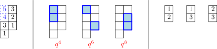
Figure 1. The hook-lengths of the skew shape $\lambda/\mu=(2^{3}1/1^{2})$, three excited diagrams for $(2^{3}1/1^{2})$ and the corresponding flagged tableaux in $\mathcal{F}(\mu,(3,3))$.

For the $q$-analogue, let

$$a(D)\,:=\,\sum_{(i,j)\in[\lambda]\setminus D}\hskip 1.70709pt(\lambda^{\prime}_{j}-i)$$

be the sum of exponents of $q$ in the numerator of the RHS of (1.4). We have $a(D_{1})=4$, $a(D_{2})=6$ and $a(D_{3})=8$, where $D_{1},D_{2},D_{3}\in\mathcal{E}(2^{3}1/1^{2})$ are the three excited diagrams in the figure.

Now Theorem 1.4 gives

$$s_{2^{3}1/1^{2}}(1,q,q^{2},\ldots)\,=\,\frac{q^{4}}{(1-q^{3})^{2}(1-q^{2})(1-q)^{2}}\hskip 1.70709pt+\\ +\hskip 1.70709pt\frac{q^{6}}{(1-q^{4})(1-q^{3})^{2}(1-q^{2})(1-q)}\hskip 1.70709pt+\hskip 1.70709pt\frac{q^{8}}{(1-q^{5})(1-q^{4})(1-q^{3})^{2}(1-q)}\hskip 1.70709pt.$$

Compare this with the expression (2.2) for the same specialization

$$s_{2^{3}1/1^{2}}(1,q,q^{2},\ldots)\,=\frac{q^{6}+2q^{4}+2q^{3}+q^{5}+2q^{2}+q}{(1-q)(1-q^{2})(1-q^{3})(1-q^{4})(1-q^{5})}.$$

Example 3.2.

For the hook shape $(k,1^{d-1})$ we have that $f^{(k,1^{d-1})}=\binom{k+d-2}{k-1}$. By symmetry, for the skew shape $\lambda/\mu$ with $\lambda=(k^{d})$ and $\mu=((k-1)^{d-1})$, we also have $f^{\lambda/\mu}=f^{(k,1^{d-1})}$. The complements of excited diagrams of this shape are in bijection with lattice paths $\gamma$ from the cell labeled $(d,1)$ to the cell $(1,k)$. Thus $|\mathcal{E}(\lambda/\mu)|=\binom{k+d-2}{k-1}$. Here is an example with $k=d=3$:

.

Moreover, since $h(i,j)=i+j-1$ for $(i,j)\in[\lambda]$ then the NHLF, switching the LHS and RHS, states in this case:

(3.1) $$\sum_{\gamma:\,(d,1)\to(1,k)}\prod_{(i,j)\in\gamma}\frac{1}{i+j-1}=\binom{k+d-2}{k-1}\hskip 0.85355pt,$$

where $\gamma:\,(d,1)\to(1,k)$ means that $\gamma$ is a NE lattice paths between the given cells. Next we apply our first $q$-analogue to this shape. First, we have that $\hskip 0.85355pts_{k1^{d-1}}=s_{\lambda/\mu}$ [S3, Prop. 7.10.4]. Next, by [S3, Cor. 7.21.3] the principal specialization of the Schur function $\hskip 0.85355pts_{k1^{d-1}}$ equals

$$s_{k1^{d-1}}(1,q,q^{2},\ldots)\,=\,q^{\binom{d}{2}}\hskip 0.85355pt\prod_{i=1}^{k+d-1}\hskip 1.70709pt\frac{1}{1-q^{i}}\begin{bmatrix}k+d-2\\ k-1\end{bmatrix}_{q},$$

where $\begin{bmatrix}n\\ k\end{bmatrix}_{q}$ is a $q$-binomial coefficient. Second if the excited diagram $D\in\mathcal{E}(\lambda/\mu)$ corresponds to path $\gamma$ then one can show that $a(D)=\binom{n}{2}+\operatorname{area}(\gamma)$ where $\operatorname{area}(\gamma)$ is the number of cells in the $d\times k$ rectangle South East of the path $\gamma$. Putting this all together then Theorem 1.4 for shape $\lambda/\mu$ gives

(3.2) $$\left(\prod_{i=1}^{k+d-1}(1-q^{i})\right)\sum_{\gamma:(d,1)\to(1,k)}q^{\operatorname{area}(\gamma)}\prod_{(i,j)\in\gamma}\frac{1}{1-q^{i+j-1}}\,=\,\begin{bmatrix}k+d-2\\ k-1\end{bmatrix}_{q}\,.$$

In [MPP3], we show that (3.1) and (3.2) are special cases of the Racah and $q$-Racah formulas in [BGR].

3.2. NHLF from its $q$-analogue.

Next, before proving Theorem 1.4, we first show that it is a $q$-analogue of (1.2). This argument is standard; we outline it for reader’s convenience.

Proposition 3.3.

Theorem 1.4 implies the NHLF (1.2).

Proof.

Multiplying (2.2) by  $(1-q)\cdots(1-q^{n})$  and using Theorem 1.4, gives

(3.3) $$\sum_{T\in\operatorname{SYT}(\lambda/\mu)}q^{\operatorname{tmaj}(T)}\,=\,\prod_{i=1}^{n}(1-q^{i})\hskip 1.70709pt\sum_{D\in\mathcal{E}(\lambda/\mu)}\hskip 1.70709pt\prod_{(i,j)\in[\lambda]\setminus D}\frac{q^{\lambda^{\prime}_{j}-i}}{1-q^{h(i,j)}}\hskip 1.70709pt.$$

Since all excited diagrams $D\in\mathcal{E}(\lambda/\mu)$ have size $|\mu|$ then by taking the limit $q\to 1$ in (3.3), we obtain the NHLF (1.2). ∎

Theorem 1.5 is a different $q$-analogue of NHLF, as explained in Section 6.

3.3. Flagged tableaux

Excited diagrams of $\lambda/\mu$ are also equivalent to certain flagged tableaux of shape $\mu$ (see Proposition 3.6 and [Kre1, §6]) and thus the number of excited diagrams is given by a determinant (see Corollary 3.7), a polynomial in the parts of $\lambda$ and $\mu$.

In this section we relate excited diagrams with flagged tableaux. The relation is based on a map by Kreiman [Kre1, §6] (see also [KMY, §5]).

We start by stating an important property of excited diagrams that follows immediately from their construction. Given a set $D\subseteq[\lambda]$ we say that $(i,j),(i+m,j+m)\in D\cap\mathsf{d}_{k}$ for $m>0$ are consecutive if there is no other element in $D$ on diagonal $\mathsf{d}_{k}$ between them.

Definition 3.4 (Interlacing property).

Let $D\subset[\lambda]$. If $(i,j)$ and $(i+m,j+m)$ are two consecutive elements in $D\cap\mathsf{d}_{k}$ then $D$ contains an element in each diagonal $\mathsf{d}_{k-1}$ and $\mathsf{d}_{k+1}$ between columns $j$ and $j+m$.  Note that the excited diagrams in $\mathcal{E}(\lambda/\mu)$ satisfy this property by construction.

Fix a sequence ${\bf f}=(\mathsf{f}_{1},\mathsf{f}_{2},\ldots,\mathsf{f}_{\ell(\mu)})$ of weakly increasing nonnegative integers. Define $\mathcal{F}(\mu,{\bf f})$ to be the set of $T\in\operatorname{SSYT}(\mu)$, such that all entries $1\leq T_{ij}\leq\mathsf{f}_{i}$. Such tableaux are called flagged SSYT and they were first studied by Lascoux and Schützenberger [LS] and Wachs [Wac]. By the Lindström–Gessel–Viennot lemma on non-intersecting paths (see e.g. [S3, Thm. 7.16.1]), the size of $\mathcal{F}(\mu,{\bf f})$ is given by a determinant:

Proposition 3.5 (Gessel–Viennot [GV], Wachs [Wac]).

In the notation above, we have:

$$|\mathcal{F}(\mu,{\bf f})|\,=\,\det\left[h_{\mu_{i}-i+j}(1^{\mathsf{f}_{i}})\right]_{i,j=1}^{\ell(\mu)}\,=\,\det\left[\binom{\mathsf{f}_{i}+\mu_{i}-i+j-1}{\mu_{i}-i+j}\right]_{i,j=1}^{\ell(\mu)},$$

where $h_{k}(x_{1},x_{2},\ldots)$ denotes the complete symmetric function.

Given a skew shape $\lambda/\mu$, each row $i$ of $\mu$ is between the rows $k_{i-1}<i\leq k_{i}$ of two corners of $\mu$. When a corner of $\mu$ is in row $k$, let $\mathsf{f}^{\prime}_{k}$ be the last row of diagonal $\mathsf{d}_{\mu_{k}-k}$ in $\lambda$. Lastly, let ${\bf f}^{(\lambda/\mu)}$ be the vector $(\mathsf{f}_{1},\mathsf{f}_{2},\ldots,\mathsf{f}_{\ell(\mu)})$, $\mathsf{f}_{i}=\mathsf{f}^{\prime}_{k_{i}}$ where $k_{i}$ is the row of the corner of $\mu$ at or immediately after row $i$ (see Figure 2). Let $\mathcal{F}(\lambda/\mu):=\mathcal{F}(\mu,{\bf f}^{(\lambda/\mu)})$.

Let $T_{\mu}$ be the tableaux of shape $\mu$ with entries $i$ in row $i$. Note that $T_{\mu}\in\mathcal{F}(\lambda/\mu)$. We define an analogue of an excited move for flagged tableaux. A cell $(x,y)$ of $T$ in $\mathcal{F}(\lambda/\mu)$ is active if increasing $T_{x,y}$ by $1$ results in a flag SSYT tableau $T^{\prime}$ in $\mathcal{F}(\lambda/\mu)$. We call this map $T\mapsto T^{\prime}$ a flagged move and denote by $\alpha^{\prime}_{x,y}(T)=T^{\prime}$.

Next we show that excited diagrams in $\mathcal{E}(\lambda/\mu)$ are in bijection with flagged tableaux in $\mathcal{F}(\lambda/\mu)$.

Given $D\in\mathcal{E}(\lambda/\mu)$, we define $\varphi(D):=T$ as follows: Each cell $(x,y)$ of $[\mu]$ corresponds to a cell $(i_{x},j_{y})$ of $D$. We let $T$ be the tableau of shape $\mu$ with $T_{x,y}=i_{x}$. An example is given in Figure 2.

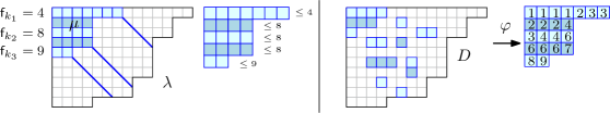
Figure 2. Given a skew shape $\lambda/\mu$, for each corner $k$ of $\mu$ we record the last row $\mathsf{f}_{k}$ of $\lambda$ from diagonal $\mathsf{d}_{\mu_{k}-k}$. These row numbers give the bound for the flagged tableaux of shape $\mu$ in $\mathcal{F}(\mu,{\bf f}^{(\lambda/\mu)})$.

Proposition 3.6.

We have $|\mathcal{E}(\lambda/\mu)|=|\mathcal{F}(\lambda/\mu)|$ and the map $\varphi$ is a bijection between these two sets.

Proof.

We need to prove that $\varphi$ is a well defined map from $\mathcal{E}(\lambda/\mu)$ to $\mathcal{F}(\mu,{\bf f}^{(\lambda/\mu)})$. First, let us show that $T=\varphi(D)$ is a SSYT by induction on the number of excited moves of $D$. First, note that $\varphi([\mu])=T_{\mu}$ which is SSYT. Next, assume that for $D\in\mathcal{E}(\lambda/\mu)$, $T=\varphi(D)$ is a SSYT and $D^{\prime}=\alpha_{(i_{x},j_{y})}(D)$ for some active cell $(i_{x},j_{y})$ of $D$ corresponding to $(x,y)$ in $[\mu]$. Then $T^{\prime}=\varphi(D^{\prime})$ is obtained from $T$ by adding $1$ to entry $T_{x,y}=i_{x}$ and leaving the rest of entries unchanged. When $(x+1,y)\in[\mu]$, since $(i_{x}+1,j_{y})$ is not in $D$ then the cell of the diagram corresponding to $(x+1,y)$ is in a row $>i_{x}+1$, therefore $T^{\prime}_{x,y}=i_{x}+1<T_{x+1,y}=T^{\prime}_{x+1,y}$. Similarly, if $(x,y+1)\in[\mu]$, since $(i_{x},j_{x}+1)$ is not in $D$ then the cell of the diagram corresponding to $(x,y+1)$ is in a row $>i_{x}$, therefore $T^{\prime}_{x,y}=i_{x}+1\leq T_{x,y+1}=T^{\prime}_{x,y+1}$. Thus, $T^{\prime}\in\operatorname{SSYT}(\lambda/\mu)$.

Next, let us show that $T$ is a flagged tableau in $\mathcal{F}(\mu,{\bf f}^{(\lambda/\mu)})$. Given an excited diagram $D$, if cell $(i_{x},j_{y})$ of $D$ is the cell corresponding to $(x,y)$ in $[\mu]$ then the row $i_{x}$ is at most $\mathsf{f}_{k_{x}}$: the last row of diagonal $\mathsf{d}_{\mu_{k_{x}}-k_{x}}$ where $k_{x}$ is the row of the corner of $\mu$ on or immediately after row $x$. Note that the numbers $\mathsf{f}_{k_{x}}$ are weakly increasing as $x$ grows, since the diagonals move to the left and so intersect $\lambda$ at lower rows. Thus $T_{x,y}\leq\mathsf{f}_{k_{x}}$, which proves the claim.

Finally, we prove that $\varphi$ is a bijection by building its inverse. Given $T\in\mathcal{F}(\mu,{\bf f}^{(\lambda/\mu)})$, let $D=\vartheta(T)$ be the set $D=\{(T_{x,y},y+T_{x,y})\mid(x,y)\in[\mu]\}$. Let us show $\vartheta$ is a well defined map from $\mathcal{F}(\mu,{\bf f}^{(\lambda/\mu)})$ to $\mathcal{E}(\lambda/\mu)$. By definition of the flags ${\bf f}^{(\lambda/\mu)}$, observe that $D$ is a subset of $[\lambda]$. We prove that $D$ is in $\mathcal{E}(\lambda/\mu)$ by induction on the number of flagged moves $\alpha^{\prime}_{x,y}(\cdot)$. First, observe that $\vartheta(T_{\mu})=[\mu]$ which is in $\mathcal{E}(\lambda/\mu)$. Assume that for $T\in\mathcal{F}(\lambda/\mu)$, $D=\vartheta(T)$ is in $\mathcal{E}(\lambda/\mu)$ and $T^{\prime}=\alpha^{\prime}_{x,y}(T)$ for some active cell $(x,y)$ of $T$. Note that replacing $T_{x,y}$ by $T_{x,y}+1$ results in a flagged tableaux $T^{\prime}$ in $\mathcal{F}(\lambda/\mu)$ is equivalent to $(i_{x},i_{y})$ being an active cell of $D$. Since $\vartheta(T^{\prime})=\alpha_{i_{x},i_{y}}(D)$ and the latter is an excited diagram, the result follows. By construction, we conclude that $\vartheta=\varphi^{-1}$, as desired. ∎

By Proposition 3.5, we immediately have the following corollary.

Corollary 3.7.

$$|\mathcal{E}(\lambda/\mu)|=\det\left[\binom{\mathsf{f}^{(\lambda/\mu)}_{i}+\mu_{i}-i+j-1}{\mathsf{f}^{(\lambda/\mu)}_{i}-1}\right]_{i,j=1}^{\ell(\mu)}.$$

Let $\mathcal{K}(\lambda/\mu)$ be the set of $T\in\operatorname{SSYT}(\mu)$ such that all entries $t=T_{i,j}$ satisfy the inequalities $t\leq\ell(\lambda)$ and $T_{i,j}+c(i,j)\leq\lambda_{t}$.

Proposition 3.8 (Kreiman [Kre1]).

We have $|\mathcal{E}(\lambda/\mu)|=|\mathcal{K}(\lambda/\mu)|$ and the map $\varphi$ is a bijection between these two sets.

Since the correspondences $\varphi$ from Propositions 3.6 and 3.8 are the same then both sets of tableaux are equal.

Corollary 3.9.

We have $\mathcal{F}(\lambda/\mu)=\mathcal{K}(\lambda/\mu)$.

Remark 3.10.

To clarify the unusual situation in this section, here we have three equinumerous sets $\mathcal{K}(\lambda/\mu)$, $\mathcal{F}(\lambda/\mu)$ and $\mathcal{E}(\lambda/\mu)$, all of which were previously defined in the literature. The first two are in fact the same sets, but defined somewhat differently; essentially, the set of inequalities in the definition of $\mathcal{K}(\lambda/\mu)$ has redundancies. Since our goal is to prove Corollary 3.7, we find it easier and more instructive to use Kreiman’s map $\varphi$ with a new analysis (see below), to prove directly that $|\mathcal{E}(\lambda/\mu)|=|\mathcal{F}(\lambda/\mu)|$. An alternative approach would be to prove the equality of sets $\mathcal{F}(\lambda/\mu)=\mathcal{K}(\lambda/\mu)$ first (Corollary 3.9), which reduces the problem to Kreiman’s result (Proposition 3.8).

4. Algebraic proof of Theorem 1.4

4.1. Preliminary results

A skew shape $\lambda/\mu$ with $\mu\subseteq\lambda\subseteq d\times(n-d)$ is in correspondence with a pair of Grassmannian permutations $w\preceq v$ of $n$ both with descent at position $d$ and where $\preceq$ is the strong Bruhat order. Recall that a permutation $v=v_{1}v_{2}\cdots v_{n}$ is Grassmannian if it has a unique descent. The permutation $v$ is obtained from the diagram $\lambda$ by writing the numbers $1,\ldots,n$ along the unit segments of the boundary of $\lambda$ starting at the bottom left corner and ending at the top right of the enclosing $d\times(n-d)$ rectangle. The permutation $v$ is obtained by first reading the $d$ numbers on the vertical segments and then the $(n-d)$ numbers on the horizontal segments. The permutation $w$ is obtained by the same procedure on partition $\mu$ (see Figure 3).

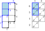
Figure 3. The skew shape $2221/11$ corresponds to the Grassmannian permutations $v=245613$ and $w=124536$.

Note that  $\bigl{(}v(1),\ldots,v(n)\bigr{)}\hskip 0.85355pt=\hskip 0.85355pt\bigl{(}\lambda_{d}+1,\lambda_{d-1}+2,\ldots\lambda_{1}+d,j_{1},\ldots,j_{n-d}\bigr{)}$  and

($$\ast v(d+1-i)\hskip 1.70709pt=\hskip 1.70709pt\lambda_{i}+d+1-i,$$)

where $\{j_{1},\ldots,j_{n-d}\}=[n]\setminus\{\lambda_{d}+1,\lambda_{d-1}+2,\ldots,\lambda_{1}+d\}$ arranged in increasing order. The numbers written up to the vertical segment on row $i$ are $1,\ldots,\lambda_{i}+d-i$, of which $d-i$ are on the first vertical segments, and the other $\lambda_{i}$ are on the first horizontal segments. This gives

($$\ast\ast \bigl{\{}v(1),\ldots,v(d-i),v(d+1),v(d+2),\ldots,v(d+\lambda_{i})\bigr{\}}\,=\,\bigl{\{}1,\ldots,\lambda_{i}+d-i\bigr{\}}\hskip 1.70709pt.$$)

Let $[X_{w}]$ be the equivariant Schubert class corresponding to a permutation $w$ and let $[X_{w}]|_{v}$ be the multivariate polynomial with variables $y_{1},\ldots,y_{n}$ corresponding to the image of the class under a certain homomorphism $\iota_{v}$. We use a result from Ikeda and Naruse [IN1] and Kreiman [Kre1] that follows from a formula by Billey for $[X_{w}]|_{v}$ when $v,w$ are Grassmannian permutations.

Theorem 4.1 (Ikeda–Naruse [IN1], Kreiman [Kre1]; Billey [Bil]).

Let $w\preceq v$ be Grassmannian permutations whose unique descent is at position $d$ with corresponding partitions $\mu\subseteq\lambda\subseteq d\times(n-d)$. Then

$$[X_{w}]\hskip 0.85355pt\bigl{|}_{v}\,\hskip 1.70709pt=\hskip 1.70709pt\sum_{D\in\mathcal{E}(\lambda/\mu)}\prod_{(i,j)\in D}\bigl{(}y_{v(d+j)}-y_{v(d-i+1)}\bigr{)}.$$

Remark 4.2.

For general permutations $w\preceq v$ the polynomial $[X_{w}]\hskip 0.85355pt\bigl{|}_{v}$ is a Kostant polynomial $\sigma_{w}(v)$, see [KK, Bil, Tym]. Billey’s formula [AJS, Appendix D.3]  [Bil, Eq. (4.5)] expresses the latter as certain sums over reduced subwords of $w$ from a fixed reduced word of $v$. Since in our context $w$ and $v$ are Grassmannian, the reduced subwords are related only by commutations and no braid relations (cf. [Ste]). This property allows the authors in [IN1, Thm. 1] to find a bijection between the reduced subwords and excited diagrams. The author in [Kre1, Prop. 2.2] uses the different method of Gröbner degenerations to prove the result.

The factorial Schur functions (see e.g. [MoS]) are defined as

$$s_{\mu}^{(d)}({\bf x}\hskip 0.85355pt|\hskip 0.85355pt{\bf a})\,:=\,\frac{\det\bigl{[}(x_{j}-a_{1})\cdots(x_{j}-a_{\mu_{i}+d-i})\bigr{]}_{i,j=1}^{d}}{\prod_{1\leq i<j\leq d}\,(x_{i}-x_{j})},$$

where $x=(x_{1},x_{2},\ldots,x_{d})$ and $a=(a_{1},a_{2},\ldots)$ is a sequence of parameters.

Theorem 4.3 (Theorem 2 in [IN1], attributed to Knutson-Tao [KT], Lakshmibai–Raghavan–Sankaran).

$$[X_{w}]\hskip 0.85355pt\bigl{|}_{v}\hskip 1.70709pt=\hskip 1.70709pt(-1)^{\ell(w)}s_{\mu}^{(d)}\bigl{(}y_{v(1)},\ldots,y_{v(d)}\hskip 0.85355pt|\hskip 0.85355pty_{1},\ldots,y_{n-1}\bigr{)}.$$

Corollary 4.4.

Let $w\preceq v$ be Grassmannian permutations whose unique descent is at position $d$ with corresponding partitions $\mu\subseteq\lambda\subseteq d\times(n-d)$. Then

(4.1) $$s_{\mu}^{(d)}\bigl{(}y_{v(1)},\ldots,y_{v(d)}\hskip 0.85355pt\bigl{|}\hskip 0.85355pty_{1},\ldots,y_{n-1}\bigr{)}\hskip 1.70709pt=\hskip 1.70709pt\sum_{D\in\mathcal{E}(\lambda/\mu)}\hskip 1.70709pt\prod_{(i,j)\in D}\bigl{(}y_{v(d-i+1)}-y_{v(d+j)}\bigr{)}.$$

Proof.

Combining Theorem 4.1 and Theorem 4.3 we get

(4.2) $$(-1)^{\ell(w)}s_{\mu}^{(d)}(y_{v(1)},\ldots,y_{v(d)}\hskip 0.85355pt\bigl{|}\hskip 0.85355pty_{1},\ldots,y_{n-1})\hskip 1.70709pt=\hskip 1.70709pt\sum_{D\in\mathcal{E}(\lambda/\mu)}\hskip 1.70709pt\prod_{(i,j)\in D}\bigl{(}y_{v(d+j)}-y_{v(d-i+1)}\bigr{)}.$$

Note that $\ell(w)=|\mu|$ and $\ell(v)=|\lambda|$, so we can remove the $(-1)^{\ell(w)}$ on the left of (4.2) by negating all linear terms on the right and get the desired result. ∎

4.2. Proof of Theorem 1.4

First we use Corollary 4.4 to get an identity of rational functions in $y=(y_{1},y_{2},\ldots,y_{n})$ (Lemma 4.5). Then we evaluate this identity at $y_{p}=q^{p-1}$ and use some identities of symmetric functions to prove the theorem. Let

$$H_{i,r}({\bf y})\,:=\,\begin{cases}\displaystyle\prod_{p=\mu_{r}+d+1-r}^{\lambda_{i}+d-i}\bigl{(}y_{\lambda_{i}+d+1-i}-y_{p}\bigr{)}^{-1}&\text{ if $\mu_{r}+d-r\leq\lambda_{i}+d-i$}\hskip 0.85355pt,\\ {\hskip 125.19194pt0}&\,\text{otherwise\hskip 0.85355pt.}\end{cases}\hskip 0.85355pt.$$

Lemma 4.5.

(4.3) $$\det\bigl{[}H_{i,j}({\bf y})\bigr{]}_{i,r=1}^{d}\hskip 1.70709pt=\hskip 1.70709pt\sum_{D\in\mathcal{E}(\lambda/\mu)}\prod_{(i,j)\in[\lambda]\setminus D}\frac{1}{y_{v(d+1-i)}-y_{v(d+j)}}.$$

Proof.

Start with (4.1) and divide both sides by

(4.4) $$\prod_{(i,j)\in[\lambda]}\bigl{(}y_{v(d+1-i)}-y_{v(d+j)}\bigl{)}\,\,=\,\prod_{i=1}^{d}\hskip 1.70709pt\prod_{j=1}^{\lambda_{i}}\hskip 1.70709pt\bigl{(}y_{v(d+1-i)}-y_{v(d+j)}\bigr{)}\hskip 1.70709pt,$$

to obtain

(4.5) $$\frac{s_{\mu}^{(d)}(y_{v(1)},\ldots,y_{v(d)}|y_{1},\ldots,y_{n-1})}{\prod_{(i,j)\in[\lambda]}(y_{v(d+1-i)}-y_{v(d+j)})}\,=\,\sum_{D\in\mathcal{E}(\lambda/\mu)}\prod_{(i,j)\in[\lambda]\setminus D}\frac{1}{y_{v(d+1-i)}-y_{v(d+j)}}.$$

Denote the LHS of (4.5) by $S_{\lambda,\mu}({\bf y})$. By the determinantal formula for factorial Schur functions and by (4.4) we have

$$S_{\lambda,\mu}({\bf y}) \,=\,\frac{\det\left[\prod_{p=1}^{\mu_{r}+d-r}(y_{v(d+1-i)}-y_{p})\right]_{i,r=1}^{d}}{\prod_{i=1}^{d}\prod_{k=i+1}^{d}(y_{v(d+1-i)}-y_{v(d+1-k)})}\cdot\frac{1}{\prod_{i=1}^{d}\prod_{j=1}^{\lambda_{i}}(y_{v(d+1-i)}-y_{v(d+j)})}$$

$$=\,\det\left[\frac{\prod_{p=1}^{\mu_{r}+d-r}(y_{v(d+1-i)}-y_{p})}{\prod_{k=i+1}^{d}(y_{v(d+1-i)}-y_{v(d+1-k)})\prod_{j=1}^{\lambda_{i}}(y_{v(d+1-i)}-y_{v(d+j)})}\right]_{i,r=1}^{d}\hskip 1.70709pt.$$

Using ($\ast\ast$ ‣ 4.1) in the denominator of the matrix entry, we obtain:

(4.6) $$S_{\lambda,\mu}({\bf y}) \hskip 1.70709pt=\hskip 1.70709pt\det\left[\prod_{p=1}^{\mu_{r}+d-r}(y_{v(d+1-i)}-y_{p})\prod_{p=1}^{\lambda_{i}+d-i}(y_{v(d+1-i)}-y_{p})^{-1}\right]_{i,r=1}^{d}.$$

By ($\ast$ ‣ 4.1), we have $v(d+1-i)=\lambda_{i}+d+1-i$. Therefore, the matrix entry on the RHS of (4.6) simplifies to $H_{i,r}({\bf y})$.

(4.7) $$S_{\lambda,\mu}({\bf y})\hskip 1.70709pt=\hskip 1.70709pt\det[H_{i,r}({\bf y})]_{i,r=1}^{d}\hskip 1.70709pt.$$

Combining (4.7) with (4.5) we obtain (4.3) as desired. ∎

Next, we evaluate $y_{p}=q^{p-1}$ for $p=1,\ldots,n$ in (4.3). Since

(4.8) $$(y_{v(d+1-i)}-y_{v(d+j)})\hskip 1.70709pt\Big{|}_{y_{p}=q^{p}}\hskip 1.70709pt=\hskip 1.70709ptq^{\lambda_{i}+d+1-i}-q^{d-\lambda_{j}^{\prime}+j}\hskip 1.70709pt=\hskip 1.70709pt-q^{d-\lambda_{j}^{\prime}+j}(1-q^{h(i,j)})\hskip 1.70709pt,$$

we obtain

(4.9) $$\det\bigl{[}H_{i,r}(1,q,q^{2},\ldots,q^{n-1})\bigr{]}_{i,r=1}^{d}\,=\,(-1)^{|\lambda|-|\mu|}\sum_{D\in\mathcal{E}(\lambda/\mu)}\hskip 1.70709pt\prod_{(i,j)\in[\lambda]\setminus D}\hskip 1.70709pt\frac{q^{-d+\lambda^{\prime}_{j}-j}}{1-q^{h(i,j)}}\hskip 1.70709pt.$$

We now simplify the matrix entry $H_{i,r}(1,q,q^{2},\ldots,q^{n-1})$. For $\nu=(\nu_{1},\ldots,\nu_{d})$, let

$$g(\nu)\hskip 1.70709pt:=\hskip 1.70709pt\sum_{i=1}^{d}\binom{\nu_{i}+d+1-i}{2}\hskip 1.70709pt.$$

We then have:

Proposition 4.6.

$$H_{i,r}(1,q,q^{2},\ldots,q^{n-1})\,=\,q^{-\binom{\lambda_{i}+d+1-i}{2}+\binom{\mu_{r}+d+1-r}{2}}\hskip 0.85355pth_{\lambda_{i}-i-\mu_{r}+r}(1,q,q^{2},\ldots)\hskip 1.70709pt,$$

where $h_{k}({\bf x})$ denotes the $k$-th complete symmetric function.

Proof.

We have:

$$H_{i,r}(1,q,q^{2},\ldots,q^{n-1}) \,=\,\prod_{p=\mu_{r}+d+1-r}^{\lambda_{i}+d-i}\hskip 1.70709pt\frac{1}{q^{\lambda_{i}+d+1-i}-q^{p}}$$

$$\,=\,(-1)^{\lambda_{i}-i-\mu_{r}+r}\hskip 1.70709ptq^{-\binom{\lambda_{i}+d+1-i}{2}+\binom{\mu_{r}+d+1-r}{2}}\hskip 1.70709pt\prod_{p=1}^{\lambda_{i}-i-\mu_{r}+r}\hskip 1.70709pt\frac{1}{1-q^{p}}$$

$$\,=\,(-1)^{\lambda_{i}-i-\mu_{r}+r}\hskip 1.70709ptq^{-\binom{\lambda_{i}+d+1-i}{2}+\binom{\mu_{r}+d+1-r}{2}}\hskip 1.70709pth_{\lambda_{i}-i-\mu_{r}+r}(1,q,q^{2},\ldots)\hskip 0.85355pt,$$

where the last identity follows by the principal specialization of the complete symmetric function. ∎

Using Proposition 4.6, the LHS of (4.9) becomes

(4.10) $$\det\bigl{[}H_{i,r}(1,q,\ldots,q^{n-1})\bigr{]}_{i,r=1}^{d} \,=\,(-1)^{|\lambda|-|\mu|}q^{-g(\lambda)+g(\mu)}\det\left[h_{\lambda_{i}-i-\mu_{r}+r}(1,q,q^{2},\ldots)\right]_{i,r=1}^{d}$$

$$\,=\,(-1)^{|\lambda|-|\mu|}q^{-g(\lambda)+g(\mu)}s_{\lambda/\mu}(1,q,q^{2},\ldots)\hskip 1.70709pt,$$

where the last equality follows by the Jacobi–Trudi identity for skew Schur functions (2.1). From here, rearranging powers of $q$ and cancelling signs, equation (4.9) becomes

(4.11) $$s_{\lambda/\mu}(1,q,q^{2},\ldots)\,=\,q^{g(\lambda)-g(\mu)}\sum_{D\in\mathcal{E}(\lambda/\mu)}\prod_{(i,j)\in[\lambda]\setminus D}\frac{q^{-d+\lambda_{j}^{\prime}-j}}{1-q^{h(i,j)}}\,.$$

It remains to match the powers of $q$ in (4.11) and (1.4).

Proposition 4.7.

For an excited diagram $D\in\mathcal{E}(\lambda/\mu)$ we have:

$$g(\lambda)-g(\mu)+\sum_{(i,j)\in[\lambda]\setminus D}(-d+\lambda^{\prime}_{j}-j)\ =\,\sum_{(i,j)\in[\lambda]\setminus D}(\lambda^{\prime}_{j}-i)\hskip 1.70709pt.$$

Proof.

Note that  $g(\lambda)=\sum_{i=1}^{d}\sum_{p=1}^{\lambda_{i}+d-i}p=\sum_{i=1}^{d}i(d-i)+d|\lambda|+\sum_{(i,j)\in[\lambda]}c(i,j)$,  where $c(i,j)=j-i$. Therefore,

$$g(\lambda)-g(\mu)-\sum_{(i,j)\in[\lambda]\setminus D}d\ =\,g(\lambda)-g(\mu)-d(|\lambda|-|D|)\,=\,\sum_{(i,j)\in[\lambda]}c(i,j)-\sum_{(i,j)\in[\mu]}c(i,j)\hskip 1.70709pt.$$

Finally, notice that the cells of any excited diagram $D$ have the same multiset of content values, since every excited move is along a diagonal and the content of the moved cell $j-i$ remains constant. Thus the power of $q$ for each term becomes

$$\sum_{(i,j)\in[\lambda]\setminus[\mu]}c(i,j)+\sum_{(i,j)\in[\lambda]\setminus D}(\lambda^{\prime}_{j}-j)=\sum_{(i,j)\in[\lambda]\setminus D}\left(c(i,j)+\lambda^{\prime}_{j}-j\right)\hskip 1.70709pt=\hskip 1.70709pt\sum_{(i,j)\in[\lambda]\setminus D}\lambda^{\prime}_{j}-i\hskip 1.70709pt,$$

as desired. ∎

Using Proposition 4.7 on the RHS of (4.11) yields (1.4) finishing the proof of Theorem 1.4.

5. The Hillman–Grassl and the RSK correspondences

5.1. The Hillman–Grassl correspondence

Recall the  Hillman–Grassl correspondence which defines a map between RPP $\pi$ of shape $\lambda$ and arrays $A$ of nonnegative integers of shape $\lambda$ such that $|\pi|=\sum_{u\in[\lambda]}A_{u}h(u)$. Let $\mathcal{A}(\lambda)$ be the set of such arrays. The weight $\omega(A)$ of $A$ is the sum $\omega(A):=\sum_{u\in\lambda}A_{u}h(u)$. We review this construction and some of its properties (see [S3, §7.22] and [Sag2, §4.2]). We denote by $\Phi$ the Hillman–Grassl map $\Phi:\pi\mapsto A$.

Definition 5.1 (Hillman–Grassl map $\Phi$).

Given a reverse plane partition $\pi$ of shape $\lambda$, let $A$ be an array of zeroes of shape $\lambda$. Next we find a path $\mathsf{p}$ of North and East steps in $\pi$ as follows:

• Start $\mathsf{p}$ with the most South-Western nonzero entry in $\pi$. Let $c_{s}$ be the column of such an entry.

• If $\mathsf{p}$ has reached $(i,j)$ and $\pi_{i,j}=\pi_{i-1,j}>0$ then $\mathsf{p}$ moves North to $(i-1,j)$, otherwise if $0<\pi_{i,j}<\pi_{i-1,j}$ then $\mathsf{p}$ moves East to $(i+1,j)$.

• The path $\mathsf{p}$ terminates when the previous move is not possible in a cell at row $r_{f}$.

Let $\pi^{\prime}$ be obtained from $\pi$ by subtracting $1$ from every entry in $\mathsf{p}$. Note that $\pi^{\prime}$ is still a RPP. In the array $A$ we add $1$ in position $A_{c_{s},r_{f}}$ and obtain array $A^{\prime}$. We iterate these three steps until we reach a plane partition of zeroes. We map $\pi$ to the final array $A$.

Theorem 5.2 ([HiG]).

The map $\Phi:\operatorname{RPP}(\lambda)\to\mathcal{A}(\lambda)$ is a bijection.

Note that if $A=\Phi(\pi)$ then $|\pi|=\omega(A)$ so as a corollary we obtain (1.5). Let us now describe the inverse $\Omega:A\mapsto\pi$ of the Hillman–Grassl map.

Definition 5.3 (Inverse Hillman–Grassl map $\Phi^{-1}$).

Given an array $A$ of nonnegative integers of shape $\lambda$, let $\pi$ be the RPP of shape $\lambda$ of all zeroes. Next, we order the nonzero entries of $A$, counting multiplicities, with the order $(i,j)<(i^{\prime},j^{\prime})$ if $j>j^{\prime}$ or $j=j^{\prime}$ and $i<i^{\prime}$ (i.e. $(i,j)$ is right of $(i^{\prime},j^{\prime})$ or higher in the same column). Next, for each entry $(r_{s},c_{j})$ of $A$ in this order $(i_{1},j_{1}),\ldots,(i_{m},j_{m})$ we build a reverse path $\mathsf{q}$ of South and West steps in $\pi$ starting at row $r_{s}$ and ending in column $c_{f}$ as follows:

• Start $\mathsf{q}$ with the most Eastern entry of $\pi$ in row $r_{s}$.

• If $\mathsf{q}$ has reached $(i,j)$ and $\pi_{i,j}=\pi_{i+1,j}$ then $\mathsf{q}$ moves South to $(i-1,j)$, otherwise $\mathsf{q}$ moves West to $(i+1,j)$.

• Path $\mathsf{q}$ ends when it reaches the Southern entry of $\pi$ in column $c_{f}$.

Step (iii) is actually attained (see e.g. [Sag2, Lemma 4.2.4]). Let $\pi^{\prime}$ be obtained from $\pi$ by adding $1$ from every entry in $\mathsf{q}$. Note that $\pi^{\prime}$ is still a RPP. In the array $A$ we subtract $1$ in position $A_{c_{f},r_{s}}$ and obtain array $A^{\prime}$. We iterate this process following the order of the nonzero entries of $A$ until we reach an array of zeroes. We map $A$ to the final RPP $\pi$. Note that $\omega(A)=|\pi|$.

Theorem 5.4 ([HiG]).

We have $\Omega=\Phi^{-1}$.

By abuse of notation, if $\pi$ is a skew RPP of shape $\lambda/\mu$, we define $\Phi(\pi)$ to be $\Phi(\hat{\pi})$ where $\hat{\pi}$ is the RPP of shape $\lambda$ with zeroes in $\mu$ and agreeing with $\pi$ in $\lambda/\mu$:

Recall that unlike for straight shapes, the enumeration of SSYT and RPP of skew shape are not equivalent. Therefore, the image $\Phi(\operatorname{SSYT}(\lambda/\mu))$ is a strict subset of $\Phi(\operatorname{RPP}(\lambda/\mu))$. In Section 7 we characterize the SSYT case in terms of excited diagrams, and in Section 6 we characterize the RPP case in terms of new diagrams called pleasant diagrams. Both characterizations require a few properties of $\Phi$ that we review next.

5.2. The Hillman–Grassl correspondence and Greene’s theorem

In this section we review key properties of the Hillman–Grassl correspondence related to the RSK correspondence [S3, §7.11]. We denote the RSK correspondence by  $\Psi:M\mapsto(P,Q)$, where $M$ is a matrix with nonnegative integer entries and $I(\Psi(M)):=P$, $R(\Psi(M)):=Q$ are SSYT of the same shape called the insertion and recording tableau, respectively.

Given a reverse plane partition $\pi$ and an integer $k$ with $1-\ell(\lambda)\leq k\leq\lambda_{1}-1$, a $k$-diagonal is the sequence of entries $(\pi_{ij})$ with $i-j=k$. Each $k$-diagonal of $\pi$ is nonincreasing and so we denote it by a partition $\nu^{(k)}$. The $k$-trace of $\pi$ denoted by $\mathrm{tr}_{k}(\pi)$ is the sum of the parts of $\nu^{(k)}$. Note that the $0$-trace of $\pi$ is the standard trace $\mathrm{tr}(\pi)=\sum_{i}\pi_{i,i}$.

Given the Young diagram of $\lambda$ and an integer $k$ with $1-\ell(\lambda)\leq k\leq\lambda_{1}-1$, let $\square_{k}^{\lambda}$ be the largest $i\times(i+k)$ rectangle that fits inside the Young diagram starting at $(1,1)$. For $k=0$, the rectangle $\square_{0}^{\lambda}=\square^{\lambda}$ is the (usual) Durfee square of $\lambda$. Given an array $A$ of shape $\lambda$, let $A_{k}$ be the subarray of $A$ consisting of the cells inside $\square^{\lambda}_{k}$ and $|A_{k}|$ be the sum of its entries. Also, given a rectangular array $B$, let ${B}^{\updownarrow}$ and ${B}^{\leftrightarrow}$ denote the arrays $B$ flipped vertically and horizontally, respectively. Here vertical flip means that the bottom row become the top row, and horizontal means that the rightmost column becomes the leftmost column.

In the construction $\Phi^{-1}$, entry $1$ in position $(i,j)$ adds $1$ to the $k$-trace if and only if $(i,j)\in\square^{\lambda}_{k}$. This observation implies the following result.

Proposition 5.5 (Gansner, Thm. 3.2 in [G1]).

Let $A=\Phi(\pi)$ then for $k$ with $1-\ell(\lambda)\leq k\leq\lambda_{1}-1$ we have

$$\mathrm{tr}_{k}(\pi)=|A_{k}|.$$

As a corollary, when $k=0$, Proposition 5.5 gives Gansner’s formula (1.7) for the generating series for $\operatorname{RPP}(\lambda)$ by size and trace. Indeed, the generating function for the arrays is a product over cells $(i,j)\in[\lambda]$ of terms which contain $t$ in the numerator if only if $(i,j)\in\square^{\lambda}$. We refer to [G1] for the details.

Let us note that not only is the $k$-trace determined by Proposition 5.5 but also the parts of $\nu^{(k)}$. This next result states that the partition $\nu^{(k)}$ and its conjugate are determined by nondecreasing and nonincreasing chains in the rectangle $A_{k}$.

Given an $m\times n$ array $M=(m_{ij})$ of nonnegative integers, an ascending chain of length $s$ of $M$ is a sequence $\mathfrak{c}:=\left((i_{1},j_{1}),(i_{2},j_{2}),\ldots,(i_{s},j_{s})\right)$ where $m\geq i_{1}\geq\cdots\geq i_{s}\geq 1$ and $1\leq j_{1}\leq\cdots\leq j_{s}\leq n$ where $(i,j)$ appears in $\mathfrak{c}$ at most $m_{ij}$ times. A descending chain of length $s$ is a sequence $\mathfrak{d}:=\left((i_{1},j_{1}),(i_{2},j_{2}),\ldots,(i_{s},j_{s})\right)$ where $1\leq i_{1}<\cdots<i_{s}\leq m$ and $1\leq j_{1}<\cdots<j_{s}\leq n$ where $(i,j)$ appears in $\mathfrak{d}$ only if $m_{ij}\neq 0$.

Let $ac_{1}(M)$ and $dc_{1}(M)$ be the length of the longest ascending and descending chains in $M$ respectively. In general for $t\geq 1$, let $ac_{t}(M)$ be the maximum combined length of $t$ ascending chains where the combined number of times $(i,j)$ appears is $m_{ij}$. We define $dc_{t}(M)$ analogously for descending chains.

Theorem 5.6 (Part (i) by Hillman–Grassl [HiG], part (ii) by Gansner [G1]).

Let $\pi\in\operatorname{RPP}(\lambda)$ and let $1-\ell(\lambda)\leq k\leq\lambda_{1}-1$. Denote by $\nu=\nu^{(k)}$ the partition whose parts are the entries on the $k$-diagonal of $\pi$, and let $A=\Phi(\pi)$. Then, for all $t\geq 1$ we have:

• $ac_{t}(A_{k})=\nu_{1}+\nu_{2}+\cdots+\nu_{t}$,

• $dc_{t}(A_{k})=\nu^{\prime}_{1}+\nu^{\prime}_{2}+\cdots+\nu^{\prime}_{t}$.

Remark 5.7.

This result is the analogue of Greene’s theorem for the RSK correspondence $\Psi$, see e.g. [S3, Thm. A.1.1.1]. In fact, we have the following explicit connection with RSK.

Corollary 5.8.

Let $\pi$ be in $\operatorname{RPP}(\lambda)$, $A=\Phi(\pi)$, and let $k$ be an integer $1-\ell(\lambda)\leq k\leq\lambda_{1}-1$. Denote by $\nu^{(k)}$ is the partition obtained from the $k$-diagonal of $\pi$. Then the shape of the tableaux in $\Psi({A_{k}}^{\updownarrow})$ and $\Psi({A_{k}}^{\leftrightarrow})$ is equal to $\nu^{(k)}$.

Example 5.9.

Let $\lambda=(4,4,3,1)$ and $\pi\in\operatorname{RPP}(\lambda)$ be as below. Then we have:

$$\pi=\ytableau*(green)0&*(yellow)134\\ 1*(green)3*(yellow)56\\ 36*(green)7\\ 3\qquad A=\Phi(\pi)=\ytableau 0&211\\ 1112\\ 211\\ 0$$

Note that $\nu^{(0)}=(7,3)$ and indeed $\ell(\nu^{(0)})=2=dc_{1}(A_{0})$. For example, take $\mathfrak{d}=\{(2,2),(3,3)\}$. Similarly, $\nu^{(1)}=(5,1)$, $\ell(\nu^{(1)})=2=dc_{1}(A_{1})$. Applying RSK to ${A_{1}}^{\leftrightarrow}$ and ${A_{0}}^{\leftrightarrow}$ we get tableaux of shape $\nu^{(1)}$ and $\nu^{(0)}$, respectively:

$$I(\Psi({A_{1}}^{\leftrightarrow}))=I(\Psi\ytableau 1&20\\ 111)=\ytableau 1&1223\\ 2\,,\qquad\ \ I(\Psi({A_{0}}^{\leftrightarrow}))=I(\Psi\ytableau 1&20\\ 111\\ 112)=\ytableau 1&112233\\ 223.$$

6. Hillman–Grassl map on skew RPP

In this section we show that the Hillman–Grassl map is a bijection between RPP of skew shape and arrays of nonnegative integers with support on certain diagrams related to excited diagrams.

6.1. Pleasant diagrams

We identify any diagram $S$ (set of boxes in $[\lambda]$) with its corresponding $0$-$1$ indicator array, i.e. array of shape $\lambda$ and support $S$.

Definition 6.1 (Pleasant diagrams).

A diagram $S\subset[\lambda]$ is a pleasant diagram of $\lambda/\mu$ if for all integers $k$ with $1-\ell(\lambda)\leq k\leq\lambda_{1}-1$, the subarray $S_{k}:=S\cap\square^{\lambda}_{k}$ has no descending chain bigger than the length $s_{k}$ of the diagonal $\mathsf{d}_{k}$ of $\lambda/\mu$, i.e. for every $k$ we have $dc_{1}(S_{k})\leq s_{k}$. We denote the set of pleasant diagrams of $\lambda/\mu$ by $\mathcal{P}(\lambda/\mu)$.

Example 6.2.

The skew shape $(2^{2}/1)$ has $12$ pleasant diagrams of which two are complements of excited diagrams (the first in each row):

.

These are diagrams $S$ of $[2^{2}]$ where $S\cap\square^{\lambda}_{-1},S\cap\square^{\lambda}_{0}$ and $S\cap\square^{\lambda}_{1}$ have no descending chain bigger than $s_{k}=|\mathsf{d}_{k}|=1$ for $k$ in $\{-1,0,1\}$.

Theorem 6.3.

A RPP $\pi$ of shape $\lambda$ has support in a skew shape $\lambda/\mu$ if and only if the support of $\Phi(\pi)$ is a pleasant diagram in $\mathcal{P}(\lambda/\mu)$. In particular

(6.1) $$\sum_{\pi\in\operatorname{RPP}(\lambda/\mu)}q^{|\pi|}=\sum_{S\in\mathcal{P}(\lambda/\mu)}\left[\prod_{u\in S}\frac{q^{h(u)}}{1-q^{h(u)}}\right].$$

Proof.

By Theorem 5.6, a RPP $\pi$ of shape $\lambda$ has support in the skew shape $\lambda/\mu$ if and only if $A=\Phi(\pi)$ satisfies

$$dc_{1}(A_{k})=\nu^{\prime}_{1}\leq s_{k},$$

for $1-\ell(\lambda)\leq k\leq\lambda_{1}-1$, where $\nu=\nu^{(k)}$. In other words, $\pi$ has support in the skew shape $\lambda/\mu$ if and only if the support $S\subseteq[\lambda]$ of $A$ is in $\mathcal{P}(\lambda/\mu)$. Thus, the Hillman–Grassl map is a bijection between $\operatorname{RPP}(\lambda/\mu)$ and arrays of nonnegative integers of shape $\lambda$ with support in a pleasant diagram $S\in\mathcal{P}(\lambda/\mu)$. This proves the first claim. Equation (6.1) follows since $|\pi|=\omega(\Phi(\pi))$. ∎

Remark 6.4.

The proof of Theorem 6.3 gives an alternative description for pleasant diagrams $\mathcal{P}(\lambda/\mu)$ as the supports of $0$-$1$ arrays $A$ of shape $\lambda$ such that $\Phi^{-1}(A)$ is in $\operatorname{RPP}(\lambda/\mu)$.

We also give a generalization of the trace generating function (1.7) for these reverse plane partitions.

Proof of Theorem 1.7.

Given a pleasant diagram $S\in\mathcal{P}(\lambda/\mu)$, let $\mathcal{B}_{S}$ be the collection of arrays of shape $\lambda$ with support in $S$. Given a RPP $\pi$, let $A=\Phi(\pi)$. By Theorem 6.3 $\pi$ has shape $\lambda/\mu$ if and only if $A$ has support in a pleasant diagram $S$ in $\mathcal{P}(\lambda/\mu)$. Thus

(6.2) $$\sum_{\pi\in\operatorname{RPP}(\lambda/\mu)}\hskip 1.70709ptq^{|\pi|}\hskip 0.85355ptt^{\mathrm{tr}(\pi)}\,\,=\,\sum_{S\in\mathcal{P}(\lambda/\mu)}\,\sum_{\pi\in\Phi^{-1}(\mathcal{B}_{S})}\hskip 1.70709ptq^{|\pi|}\hskip 0.85355ptt^{\mathrm{tr}(\pi)}\,,$$

where for each $S\in\mathcal{P}(\lambda/\mu)$ we have

(6.3) $$\sum_{\pi\in\Phi^{-1}(\mathcal{B}_{S})}\hskip 1.70709ptq^{|\pi|}\,=\,\prod_{u\in S}\frac{q^{h(u)}}{1-q^{h(u)}}\,.$$

Next, by Proposition 5.5 for $k=0$, the trace $\mathrm{tr}(\pi)$ equals $|A_{0}|$, the sum of the entries of $A$ in the Durfee square $\square^{\lambda}$ of $\lambda$. Therefore, we refine (6.3) to keep track of the trace of the RPP and obtain

(6.4) $$\sum_{\pi\in\Phi^{-1}(\mathcal{B}_{S})}\hskip 1.70709ptq^{|\pi|}\hskip 0.85355ptt^{\mathrm{tr}(\pi)}\,=\,\prod_{u\in S\cap\square^{\lambda}}\frac{t\hskip 0.85355ptq^{h(u)}}{1-t\hskip 0.85355ptq^{h(u)}}\,\prod_{u\in S\setminus\square^{\lambda}}\hskip 1.70709pt\frac{q^{h(u)}}{1-q^{h(u)}}\,.$$

Combining (6.2) and (6.4) gives the desired result. ∎

6.2. Combinatorial proof of NHLF (1.2): relation between pleasant and excited diagrams.

Theorem 1.4 relates SSYT of skew shape with excited diagrams and Theorem 6.3 relates RPP of skew shape with pleasant diagrams. Since SSYT are RPP then we expect a relation between pleasant and excited diagrams of a fixed skew shape $\lambda/\mu$. The first main result of this subsection characterizes the pleasant diagrams of maximal size in terms of excited diagrams. The second main result characterizes all pleasant diagrams.

The key towards these results is a more graphical characterization of pleasant diagrams as described in the proof of Lemma 6.6. It makes the relationship with excited diagrams more apparent and also allows for a more intuitive description for both kinds of diagrams.

Theorem 6.5.

A pleasant diagram $S\in\mathcal{P}(\lambda/\mu)$ has size $|S|\leq|\lambda/\mu|$ and has maximal size $|S|=|\lambda/\mu|$ if and only if the complement $[\lambda]\setminus S$ is an excited diagram in $\mathcal{E}(\lambda/\mu)$.

By combining this theorem with Theorem 6.3 we derive again the NHLF. In contrast with the derivation of this formula in Proposition 3.3 (our first proof of the NHLF), this derivation is entirely combinatorial.

Second proof of the NHLF (1.2).

By Stanley’s theory of $P$-partitions, [S3, Thm. 3.15.7]

(6.5) $$\sum_{\pi\in\operatorname{RPP}(\lambda/\mu)}q^{|\pi|}\,=\,\frac{\sum_{w\in\mathcal{L}(P_{\lambda/\mu})}\,q^{\operatorname{maj}(w)}}{\prod_{i=1}^{n}(1-q^{i})}\,,$$

where $n=|\lambda/\mu|$ and the sum in the numerator of the RHS is over linear extensions $w$ of the poset $P_{\lambda/\mu}$ with a natural labelling. Multiplying (6.5) by $(1-q)\cdots(1-q^{n})$, and using Theorem 1.5 gives

(6.6) $$\sum_{w\in\mathcal{L}(P_{\lambda/\mu})}q^{\operatorname{maj}(w)}\,=\,\left(\prod_{i=1}^{n}(1-q^{i})\right)\sum_{S\in\mathcal{P}(\lambda/\mu)}\hskip 1.70709pt\prod_{u\in S}\hskip 1.70709pt\frac{q^{h(u)}}{1-q^{h(u)}}\hskip 1.70709pt.$$

By Theorem 6.5, pleasant diagrams $S\in\mathcal{P}(\lambda/\mu)$ have size $|S|\leq n$, with the equality here exactly when $\overline{S}\in\mathcal{E}(\lambda/\mu)$. Thus, letting  $q\to 1$  in (6.6) gives $f^{\lambda/\mu}$ on the LHS. On the RHS, we obtain the sum of products

$$\prod_{u\in\overline{S}}\hskip 1.70709pt\frac{1}{h(u)}\,,$$

over all excited diagrams $S\in\mathcal{E}(\lambda/\mu)$. This implies the NHLF (1.2). ∎

Lemma 6.6.

Let  $S\in\mathcal{P}(\lambda/\mu)$. Then there is an excited diagram $D\in\mathcal{E}(\lambda/\mu)$, such that  $S\subseteq[\lambda]\setminus D$.

Proof.

Given a pleasant diagram $S$, we use Viennot’s shadow lines construction [Vie] to obtain a family of nonintersecting paths on $[\lambda]$. That is, we imagine there is a light source at the $(1,1)$ corner of $[\lambda]$ and the elements of $S$ cast shadows along the axes with vertical and horizontal segments. The boundary of the resulting shadow forms the first shadow line $L_{1}$. If lines $L_{1},L_{2},\ldots,L_{i-1}$ have already been defined we define $L_{i}$ inductively as follows: remove the elements of $S$ contained in any of the $i-1$ lines and set $L_{i}$ to be the shadow line of the remaining elements of $S$. We iterate this until no element of $S$ remains in the shadows. Let $L_{1},L_{2},\ldots,L_{m}$ be the shadow lines produced. Note that these lines form $m$ nonintersecting paths in $[\lambda]$ that go from bottom south-west cells of columns to rightmost north-east cells of rows of the diagram.

By construction, the peaks (i.e. top corners) of the shadow lines $L_{i}$ are elements of $S$ while other cells of $L_{i}$ might be in $[\lambda]\setminus S$.

Next, we augment $S$ to obtain $S^{*}$ by adding all the cells of lines $L_{1},\ldots,L_{m}$ that are not in $S$. Note that $S^{*}$ is also a pleasant diagram in $\mathcal{P}(\lambda/\mu)$ since the added cells of the lines $L_{1},\ldots,L_{m}$ do not yield longer decreasing chains than those in $S$. Moreover, no two cells from a decreasing chain can be part of the same shadow line, and there is at least one decreasing subsequence with cells in all lines, as can be constructed by induction. In particular, the number of shadow lines intersecting each diagonal $\mathsf{d}_{k}$ (i.e. intersecting the rectangle $\square^{\lambda}_{k}$) is at most $s_{k}$. Denote this number by $s^{\prime}_{k}$.

Next, we claim that $S^{*}$ is the complement of an excited diagram $D^{*}\in\mathcal{E}(\lambda/\nu)$ for some partition $\nu$. To see this we do moves on the noncrossing paths (shadow lines) that are analogous to reverse excited moves, as follows. If the lines contain $(i,j),(i+1,j),(i,j+1)$ but not $(i+1,j+1)$, then notice that the first three boxes lie on one path $L_{t}$. In this path we replace $(i,j)$ with $(i+1,j+1)$ to obtain path $L^{\prime}_{t}$. We do the same replacement in $S^{*}$:

Following Kreiman [Kre1, §5] we call this move a reverse ladder move. By doing reverse ladder moves iteratively on $S^{*}$ we obtain the complement of some Young diagram $[\nu]\subseteq[\lambda]$.

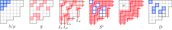
Figure 4. Example of the construction in Lemma 6.6. From left to right: a shape $\lambda/\mu$, a pleasant diagram $S\in\mathcal{P}(\lambda/\mu)$, the shadow lines associated to $S$, the augmented pleasant diagram $S^{*}$ that is a complement of an excited diagram $D^{*}$ in $\mathcal{E}(\lambda/\nu)$ for some $\nu$, $\mu\subseteq\nu\subseteq\lambda$. In general, $D^{*}$ contains all $D\in\mathcal{E}(\lambda/\mu)$ with $S\subseteq[\lambda]\setminus D$.

Next, we show that $\mu\subseteq\nu$. Reverse ladder moves do not change the number $s^{\prime}_{k}$ of shadow lines intersecting each diagonal, thus $s^{\prime}_{k}$ is also the length of the diagonal $\mathsf{d}_{k}$ of $\lambda/\nu$. Since $s^{\prime}_{k}\leq s_{k}$, the length of the diagonal $\mathsf{d}_{k}$ of $\lambda/\mu$, then $\mu\subseteq\nu$ as desired.

Finally, we have  $D^{*}=[\lambda]\setminus S^{*}$ is in $\mathcal{E}(\lambda/\nu)$, since the reverse ladder move is the reverse excited move on the corresponding diagram. Since $D^{*}$ is obtained my moving the cells of $[\nu]$ we can consider the cells of $D^{*}$ which correspond to the cells of $[\mu]\subseteq[\nu]$, denote the collection of these cells as $D$. Then $D\in\mathcal{E}(\lambda/\mu)$, and we have:

$$S\subseteq S^{*}=[\lambda]\setminus D^{*}\subseteq[\lambda]\setminus D$$

and the statement follows. ∎

We prove Theorem 6.5 via three lemmas.

Lemma 6.7.

For all  $D\in\mathcal{E}(\lambda/\mu)$, we have  $[\lambda]\setminus D\in\mathcal{P}(\lambda/\mu)$.

Proof.

Let $D_{0}=\mu$, i.e. the excited diagram which corresponds to the original skew shape $\lambda/\mu$. Following the shadow line construction from the proof of Lemma 6.6, we construct the shadow lines for the diagram $P_{0}=[\lambda/\mu]$. These lines trace out the rim-hook tableaux: let $L_{1}$ be the outer boundary of $[\mu]$ inside $[\lambda]$, then $L_{2}$ is the outer boundary of what remains after removing $L_{1}$, etc. If the skew shape becomes disconnected then there are separate lines for each connected segment.

Since a diagonal of length $\ell$ has exactly $\ell$ shadow lines crossing it, we have for each rectangle $D_{k}$ there are exactly $s_{k}$ lines $L_{i}$ crossing $\mathsf{d}_{k}$ and hence also crossing $D_{k}$. An excited move corresponds to a ladder move on some line (see the proof of Lemma 6.6), which makes an inner corner of a line into an outer corner. These moves cannot affect the endpoints of a line, so if a line does not cross a rectangle $D_{k}$ initially then it will never cross it after any number of excited moves. Moreover, any diagonal $\mathsf{d}_{k}$ will be crossed by the same set of lines formed originally in $P_{0}$. Hence the complement of any excited diagram is a collection of shadow lines, which were obtained from the original ones by ladder moves. Then the number of shadow lines crossing $D_{k}$ is always $s_{k}$. Finally, since no decreasing sequence can have more than one box on a given shadow line (i.e., a SW to NE lattice path), we have the longest decreasing subsequence in $D_{k}$ will have length at most $s_{k}$ – the number of shadow lines there. Therefore, the excited diagram satisfies Definition 6.1. ∎

By Lemma 6.7, the complements of excited diagrams in $\mathcal{E}(\lambda/\mu)$ give pleasant diagrams of size $|\lambda/\mu|$. Next, we show that there are no pleasant diagrams of larger size.

Lemma 6.8.

For all  $S\in\mathcal{P}(\lambda/\mu)$, we have  $|S|\leq|\lambda/\mu|$.

Proof.

For each diagonal $\mathsf{d}_{k}$ of $\lambda/\mu$, any elements of $S\cap\mathsf{d}_{k}$ form a descending chain in $S_{k}$. Thus, by definition of pleasant diagrams $|S\cap\mathsf{d}_{k}|\leq s_{k}$ where $s_{k}=\left|[\lambda/\mu]\cap\mathsf{d}_{k}\right|$ is the length of diagonal $\mathsf{d}_{k}$ in $\lambda/\mu$. Therefore,

$$|S| \,=\,\sum_{k=1-\ell(\lambda)}^{\lambda_{1}-1}\hskip 1.70709pt|S\cap\mathsf{d}_{k}|\,\,\leq\,\sum_{k=1-\ell(\lambda)}^{\lambda_{1}-1}\hskip 1.70709pts_{k}\,=\,|\lambda/\mu|\hskip 1.70709pt,$$

as desired. ∎

The next result shows that the only pleasant diagrams of size $|\lambda/\mu|$ are complements of excited diagrams.

Lemma 6.9.

For all  $S\in\mathcal{P}(\lambda/\mu)$  with  $|S|=|\lambda/\mu|$, we have  $[\lambda]\setminus S\in\mathcal{E}(\lambda/\mu)$.

Proof.

By the argument in the proof of Lemma 6.8, if $S\in\mathcal{P}(\lambda/\mu)$ has size $|S|=|\lambda/\mu|$ then for each integer $k$ with $1-\ell(\lambda)\leq k\leq\lambda_{1}$ we have $|S\cap\mathsf{d}_{k}|=|\mathsf{d}_{k}|=s_{k}$.

Suppose $\overline{S}=[\lambda]\setminus S$ is not an excited diagram. This means that there are two cells $a=(i,j),b=(i+m,j+m)\in\overline{S}$ on some diagonal $\mathsf{d}_{k}$ with no other cell of $\mathsf{d}_{k}$ in $\overline{S}$ between them, that violate the interlacing property (Definition 3.4). This means that there are no other cells in $\overline{S}$ between cells $a$ and $b$ in either diagonal $\mathsf{d}_{k+1}$ or diagonal $\mathsf{d}_{k-1}$. Without loss of generality assume that this occurs in diagonal $\mathsf{d}_{k-1}$. This means that all the $m$ cells in $\mathsf{d}_{k-1}$ between cells $a$ and $b$ are in $S$. Let $\mathfrak{d}$ be the descending chain in $S$ of all the $s_{k}$ cells in $S\cap\mathsf{d}_{k}$ including the $m-1$ cells in $\mathsf{d}_{k}$ between $a$ and $b$. Let $\mathfrak{d}^{\prime}$ be the descending chain consisting of the cells in $S\cap\mathsf{d}_{k}$ before cell $a$, followed by the $m$ cells in $S\cap\mathsf{d}_{k-1}$ between cell $a$ and $b$, and the cells in $S\cap\mathsf{d}_{k}$ after cell $b$ (see Figure 5). However $|\mathfrak{d}^{\prime}|=s_{k}+1$ which contradicts the requirement that all descending chains in $S\cap\square^{\lambda}_{k}$ have length $\leq s_{k}$. ∎

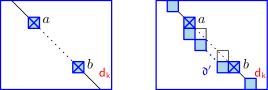
Figure 5. Two consecutive cells $a$ and $b$ in $\overline{S}$ that violate the interlacing property of excited diagrams.

Proof of Theorem 6.5.

The result follows by combining Lemmas 6.7 and 6.9. ∎

Theorem 6.10.

A diagram $S\subset[\lambda]$ is a pleasant diagram in $\mathcal{P}(\lambda/\mu)$ if and only if $S\subseteq[\lambda]\backslash D$ for some excited diagram $D\in\mathcal{E}(\lambda/\mu)$.

We need a new lemma to prove this result.

Lemma 6.11.

Given an excited diagram $D$ in $\mathcal{E}(\lambda/\mu)$ then $S\subseteq[\lambda]\backslash D$ is a pleasant diagram in $\mathcal{P}(\lambda/\mu)$.

Proof.

Theorem 6.5 characterizes maximal pleasant diagrams in $\mathcal{P}(\lambda/\mu)$ as complements of excited diagrams in $\mathcal{E}(\lambda/\mu)$. Since subsets of pleasant diagrams are also pleasant diagrams, then all subsets $S$ of $[\lambda]\setminus D$ for $D\in\mathcal{E}(\lambda/\mu)$ are pleasant diagrams. ∎

Proof of Theorem 6.10.

The theorem follows from Lemma 6.11 and Lemma 6.6. ∎

6.3. Enumeration of pleasant diagrams

Next we give two formulas for the number of pleasant diagrams of $\lambda/\mu$ as sums of excited diagrams. Both formulas are corollaries of the proof of Lemma 6.6. Given a pleasant diagram $S$, let $\operatorname{shpk}(D)$ be the number of peaks of the shadow lines $L_{1},\ldots,L_{m}$ obtained from the pleasant diagram $[\lambda]\setminus{D}$.

Proposition 6.12.

$$|\mathcal{P}(\lambda/\mu)|=\sum_{\nu,\mu\subseteq\nu\subseteq\lambda}\sum_{D\in\mathcal{E}(\lambda/\nu)}2^{|\lambda/\nu|-\operatorname{shpk}(D)}.$$

Example 6.13.

The skew shape $(2^{2}/1)$ has $12$ pleasant diagrams (see Example 6.2). The possible $\nu$ containing $\mu=(1)$ are $(1),(1^{2}),(2),(2,1),(2,2)$ and their corresponding excited diagrams with peaks (in pink) are the following:

.

We can see that $12=2^{1}+2^{2}+2^{1}+2^{1}+2^{0}+2^{0}$.

Proof of Proposition 6.12.

As in the proof of Lemma 6.6, from the shadow lines $L_{1},L_{2},\ldots,L_{m}$ of a pleasant diagram $S\in\mathcal{P}(\lambda/\mu)$ we obtain an excited diagram $D^{*}\in\mathcal{E}(\lambda/\nu)$ for $\mu\subseteq\nu$ such that $S\subseteq[\lambda]\setminus D^{*}$. The peaks of these lines are elements in $S$, and these peaks uniquely determine the lines. The other cells in the lines, $|\lambda/\nu|-\operatorname{shpk}(D^{*})$ many, may or may not be in $S$.

Therefore, we obtain a surjection

$$\varrho_{1}:\hskip 1.70709pt\mathcal{P}(\lambda/\mu)\to\bigcup_{\nu,\mu\subseteq\nu\subseteq\lambda}\mathcal{E}(\lambda/\nu)\hskip 1.70709pt,\qquad\varrho_{1}:\hskip 1.70709ptS\mapsto D^{*}\hskip 1.70709pt,$$

such that  $|\varrho_{1}^{-1}(D^{*})|=2^{|\lambda/\nu|-\operatorname{shpk}(D^{*})}$. This implies the result (see Figure 6). ∎

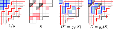
Figure 6. Example of the maps $\varrho_{1}$ and $\varrho_{2}$ on a pleasant diagram $S$.

For the second formula we need to define a similar peak statistic $\operatorname{expk}(D)$ for each excited diagram $D\in\mathcal{E}(\lambda/\mu)$. For an excited diagram $D$ we associate a subset of $[\lambda]\setminus D$ called excited peaks and denote it by $\Lambda(D)$ in the following way. For $[\mu]\in\mathcal{E}(\lambda/\mu)$ the set of excited peaks is $\Lambda([\mu])=\varnothing$. If $D$ is an excited diagram with active cell $u=(i,j)$ then the excited peaks of $\alpha_{u}(D)$ are

$$\Lambda(\alpha_{u}(D))=\left(\Lambda(D)-\{(i,j+1),(i+1,j)\}\right)\cup\{u\}.$$

That is, the excited peaks of $\alpha_{u}(D)$ are obtained from those of $D$ by adding $(i,j)$ and removing $(i,j+1)$ and $(i+1,j)$ if any of the two are in $\Lambda(D)$:

.

Finally, let $\operatorname{expk}(D):=|\Lambda(D)|$ be the number of excited peaks of $D$.

Theorem 6.14.

For a skew shape $\lambda/\mu$ we have

$$|\mathcal{P}(\lambda/\mu)|=\sum_{D\in\mathcal{E}(\lambda/\mu)}2^{|\lambda/\mu|-\operatorname{expk}(D)},$$

where $\operatorname{expk}(D)$ is the number of excited peaks of the excited diagram $D$.

We prove Theorem 6.14 via the following Lemma. Given a set $\mathcal{S}$, let $2^{\mathcal{S}}$ denote the subsets of $\mathcal{S}$.

Lemma 6.15.

We have $\mathcal{P}(\lambda/\mu)=\bigcup_{D\in\mathcal{E}(\lambda/\mu)}\Lambda(D)\times 2^{[\lambda]\setminus(D\cup\Lambda(D))}$.

Proof.

As in the proof of Lemma 6.6, from the shadow lines $L_{1},L_{2},\ldots,L_{m}$ of a pleasant diagram $S\in\mathcal{P}(\lambda/\mu)$ we obtain an excited diagram $D^{*}\in\mathcal{E}(\lambda/\nu)$ for $\mu\subseteq\nu$ such that $S\subseteq[\lambda]\setminus D^{*}$. If we restrict $D^{*}$ to the cells coming from $[\mu]$ we obtain an excited diagram $D\in\mathcal{E}(\lambda/\mu)$. Setting $\varrho_{2}(S)=D$ defines a new surjection  $\varrho_{2}:\hskip 0.85355pt\mathcal{P}(\lambda/\mu)\to\mathcal{E}(\lambda/\mu)$ (see Figure 6). It remains to prove that

$$\varrho_{2}^{-1}(D)\,=\,\Lambda(D)\times 2^{[\lambda]\setminus(D\cup\Lambda(D))}\hskip 1.70709pt.$$

First, the excited peaks are peaks of the shadow lines $L^{\prime}_{1},L^{\prime}_{2},\ldots,L^{\prime}_{k}$ of $[\lambda]\setminus D$ obtained by a ladder move:

Thus the peaks of the shadow lines $\{L^{\prime}_{i}\}$ are either excited peaks or original peaks of the shadow lines of $[\lambda/\mu]$. Second, note that the excited peaks $\Lambda(D)$ determine uniquely the excited diagram $D$. Thus the non-excited peaks of the shadow lines and the other cells of the lines $\{L^{\prime}_{i}\}$, those in $[\lambda]\setminus(D\cup\Lambda(D))$, may or may not be in $S$. This proves the claim for $\varrho_{2}^{-1}(D)$. ∎

Proof of Theorem 6.14.

By Lemma 6.15 and since $|[\lambda]\setminus(D\cup\Lambda(D))|=|\lambda/\mu|-\operatorname{expk}(D)$ then

$$|\mathcal{P}(\lambda/\mu)|=\sum_{D\in\mathcal{E}(\lambda/\mu)}2^{|\lambda/\mu|-\operatorname{expk}(D)},$$

as desired. ∎

Example 6.16.

The skew shape $(2^{2}/1)$ has $12$ pleasant diagrams (see Example 6.2) and $2$ excited diagrams, with sets of excited peaks $\varnothing$ and $\{(1,1)\}$, respectively. Indeed, we have $|\mathcal{P}(2^{2}/1)=2^{3}+2^{2}=12$. A more complicated example is shown in Figure 7. The number of pleasant diagrams in this case is $|\mathcal{P}(4^{3}/2)|=2^{10}+2\cdot 2^{9}+3\cdot 2^{8}=2816$.

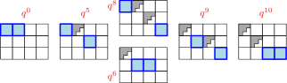
Figure 7. The six excited diagrams $D$ for $\lambda/\mu=(4^{3}/2)$, their corresponding excited peaks (in gray), and weights $a^{\prime}(D)$, defined as sums of hook-lengths of these peaks.

6.4. Excited diagrams and skew RPP

In Section 6.1 we expressed the generating function of skew RPP using pleasant diagrams. In this section we use Lemma 6.15 to give an expression for this generating series in terms of excited diagrams.

Corollary 6.17.

We have:

$$\sum_{\pi\in\operatorname{RPP}(\lambda/\mu)}q^{|\pi|}\,=\,\sum_{D\in\mathcal{E}(\lambda/\mu)}q^{a^{\prime}(D)}\prod_{u\in[\lambda]\setminus D}\frac{1}{1-q^{h(u)}}\hskip 1.70709pt,$$

where  $a^{\prime}(D):=\sum_{u\in\Lambda(D)}h(u)$.

Example 6.18.

The shape $\lambda/\mu=(4^{3}/2)$ has six excited diagrams. See Figure 7 for the corresponding statistic $a^{\prime}(D)$ of each of these diagrams.

Example 6.19.

Following Example 3.2, take the inverted hook shape  $(k^{d}/(k-1)^{d-1}$ and apply Corollary 6.17. Using Stanley’s theory of $P$-partitions, we obtain:

(6.7) $$\prod_{i=1}^{k+d-1}\frac{1}{1-q^{i}}\,{\Bigg{[}}\sum_{S\in\binom{[k+d-2]}{k-1}}q^{\operatorname{maj}(S)}{\Bigg{]}}\,=\,\sum_{\gamma:\,(d,1)\to(1,k)}q^{a^{\prime}(\gamma)}\,\prod_{(i,j)\in\gamma}\frac{1}{1-q^{i+j-1}}\,,$$

where

$$\operatorname{maj}(S)\hskip 1.70709pt=\hskip 1.70709pt\sum_{i\not\in S,i+1\in S}(i+1)\qquad\text{and}\qquad a^{\prime}(\gamma)\hskip 1.70709pt=\hskip 1.70709pt\sum_{(i,j)\text{ peak of }\gamma}\hskip 1.70709pt(i+j-1)\,.$$

The $q$-analogue of the binomial coefficients in the RHS of (6.7) appears to be new.

Proof of Corollary 6.17.

By Theorem 6.3, we have:

$$\sum_{\pi\in\operatorname{RPP}(\lambda/\mu)}q^{|\pi|}\,=\,\sum_{S\in\mathcal{P}(\lambda/\mu)}\hskip 1.70709pt\prod_{u\in S}\hskip 1.70709pt\frac{q^{h(u)}}{1-q^{h(u)}}\hskip 1.70709pt.$$

Using Lemma 6.15 and the surjection $\vartheta_{2}$ in its proof, we can rewrite the RHS above as a sum over excited diagrams. We have:

$$\sum_{S\in\mathcal{P}(\lambda/\mu)}\hskip 1.70709pt\prod_{u\in S}\hskip 1.70709pt\frac{q^{h(u)}}{1-q^{h(u)}} =\sum_{D\in\mathcal{E}(\lambda/\mu)}\hskip 1.70709pt\sum_{S\in\varrho_{2}^{-1}(D)}\hskip 1.70709pt\prod_{u\in S}\hskip 1.70709pt\frac{q^{h(u)}}{1-q^{h(u)}}$$

$$=\,\sum_{D\in\mathcal{E}(\lambda/\mu)}\hskip 1.70709pt\prod_{u\in\Lambda(D)}\hskip 1.70709ptq^{a^{\prime}(D)}\,\prod_{u\in[\lambda]\setminus D}\hskip 1.70709pt\frac{1}{1-q^{h(u)}}\hskip 1.70709pt,$$

as desired. ∎

This result also implies the NHLF (1.2).

Third proof of the NHLF (1.2).

By Stanley’s theory of $P$-partitions, [S3, Thm. 3.15.7] we obtain (6.5). Multiplying this equation by $\prod_{i=1}^{n}(1-q^{i})$ where $n=|\lambda/\mu|$ and using Corollary 6.17 gives

$$\sum_{w\in\mathcal{L}(P_{\lambda/\mu})}q^{\operatorname{maj}(w)}=\prod_{i=1}^{n}(1-q^{i})\sum_{D\in\mathcal{E}(\lambda/\mu)}q^{a^{\prime}(D)}\hskip 1.70709pt\prod_{u\in[\lambda]\setminus D}\frac{1}{1-q^{h(u)}}\hskip 1.70709pt,$$

Taking the limit $q\to 1$ in the equation above gives the NHLF (1.2). ∎

Corollary 6.20.

We have:

$$\sum_{\pi\in\operatorname{RPP}(\lambda/\mu)}\hskip 1.70709ptq^{|\pi|}\hskip 0.85355ptt^{\mathrm{tr}(\pi)}\,=\,\sum_{D\in\mathcal{E}(\lambda/\mu)}q^{a^{\prime}(D)}\hskip 0.85355ptt^{c(D)}\,\prod_{u\in\overline{D}\cap\square^{\lambda}}\frac{1}{1-t\hskip 0.85355ptq^{h(u)}}\,\prod_{u\in\overline{D}\setminus\square^{\lambda}}\frac{1}{1-q^{h(u)}}\,,$$

where  $\overline{D}=[\lambda]\setminus D$,  $a^{\prime}(D)=\sum_{u\in\Lambda(D)}h(u)$  and  $c(D)=|\Lambda(D)\cap\square^{\lambda}|$.

Proof.

The proof follows verbatim to those of Theorems 1.7, 1.8 and Corollary 6.17. The details are straightforward. ∎

7. Hillman–Grassl map on skew SSYT

In this section we show that the Hillman–Grassl map is a bijection between SSYT of skew shape and certain arrays of nonnegative integers with support in the complement of excited diagrams and some forced nonzero entries. First, we describe these arrays and state the main result. Note that in contrast with the previous section, the argument is not entirely bijective and requires Theorem 1.4 (see also $\S$9.5).

7.1. Excited arrays

We fix the skew shape $\lambda/\mu$. Recall that for $1\leq t\leq\ell(\lambda)-1$, $\mathsf{d}_{t}(\mu)$ denotes the diagonal $\{(i,j)\in\lambda/\mu\mid i-j=\mu_{t}-t\}$, where $\mu_{t}=0$ if $\ell(\mu)<t\leq\ell(\lambda)$. Thus each row of $\mu$ is in correspondence with a diagonal $\mathsf{d}_{t}(\mu)$. See Figure 8: Left.

Let $A_{\mu}$ be the array of shape $\lambda$ with ones in each diagonal $\mathsf{d}_{t}(\mu)$ and zeros elsewhere. For $[\mu]\in\mathcal{E}(\lambda/\mu)$, each active cell $u=(i,j)$ of $[\mu]$ satisfies $(A_{\mu})_{i+1,j}=0$ and $(A_{\mu})_{i+1,j+1}=1$.

For each active cell $u$ of $[\mu]$, $\alpha_{u}(D_{\mu})$ gives another excited diagram in $\mathcal{E}(\lambda/\mu)$. We do an analogous action:

(7.1) $$\beta_{u}:\,\,\raisebox{-6.0pt}{\includegraphics{excited_move_bd}}$$

on $A_{\mu}$ to obtain a $0$-$1$ array associated to $\alpha_{u}(D_{\mu})$. Concretely if $A$ is a $0$-$1$ array of shape $\lambda$ and $u=(i,j)$ is a cell such that $A_{i+1,j}=0$ and $A_{i+1,j+1}=1$ then $\beta_{u}(A)$ is the $0$-$1$ array $B$ of shape $\lambda$ with $B_{i+1,j+1}=0$, $B_{i+1,j}=1$ and $B_{v}=A_{v}$ for $v\neq\{(i+1,j),(i+1,j+1)\}$. Next, we define excited arrays by repeatedly applying $\beta_{u}(\cdot)$ on active cells $u$ starting from $A_{\mu}$.

Definition 7.1 (excited arrays).

For an excited diagram $D$ in $\mathcal{E}(\lambda/\mu)$ obtained from $[\mu]$ by a sequence of excited moves $D=\alpha_{u_{k}}\circ\alpha_{u_{k-1}}\circ\cdots\circ\alpha_{u_{1}}(\mu)$, then we let $A_{D}=\beta_{u_{k}}\circ\beta_{u_{k-1}}\circ\cdots\circ\beta_{u_{1}}(A_{\mu})$ provided the operations $\beta_{u}$ are well defined. So each excited diagram $D$ is associated to a $0$-$1$ array $A_{D}$ (see Figure 8).

Next we show that the procedure for obtaining the arrays $A_{D}$ is well defined; meaning that at each stage, the conditions to apply $\beta_{u}(\cdot)$ are met.

Proposition 7.2.

Let $A_{D}$ be the excited array of $D\in\mathcal{E}(\lambda/\mu)$ and $u=(i,j)$ be an active cell of $D$. Then $(A_{D})_{i+1,j+1}=1$ and $(A_{D})_{i+1,j}=0$.

Proof.

We prove this by induction on the number of excited moves. If $D=[\mu]$ and $u\in[\mu]$ is an active cell then $u=(t,\mu_{t})$ is the last cell of a row of $\mu$ with $\mu_{t+1}<\mu_{t}$. This implies that $(t+1,\mu_{t}+1)\in\mathsf{d}_{t}(\mu)$ and $(t+1,\mu_{t})\not\in\mathsf{d}_{t+1}(\mu)$ and so $(A_{\mu})_{t+1,\mu_{t}+1}=1$ and $(A_{\mu})_{t+1,\mu_{t}}=0$.

Assume the result holds for $D\in\mathcal{E}(\lambda/\mu)$. If $D^{\prime}=\alpha_{(i,j)}(D)$ then $A_{D^{\prime}}=\beta_{(i,j)}(A_{D})$ is well defined since $(A_{D})_{i+1,j+1}=1$ and $(A_{D})_{i+1,j}=0$. Let $v=(i^{\prime},j^{\prime})$ be an active cell of $D^{\prime}$. If $v^{\prime}=(i^{\prime},j^{\prime})$ is also an active cell of $D$, then the excited move $\beta_{u}(\cdot)$ did not alter the values at $(i^{\prime}+1,j^{\prime}+1)$ and $(i^{\prime}+1,j^{\prime})$. In this case $(A_{D^{\prime}})_{i^{\prime}+1,j^{\prime}+1}=(A_{D})_{i+1,j+1}=1$ and $(A_{D^{\prime}})_{i^{\prime}+1,j^{\prime}}=(A_{D})_{i^{\prime}+1,j^{\prime}}=0$. If $v^{\prime}$ is not an active square of $D$ then $u$ is one of $\{(i^{\prime},j+1),(i^{\prime}+1,j^{\prime}),(i^{\prime}-1,j^{\prime}-1)\}$ (note that $u\neq(i^{\prime}+1,j^{\prime}+1)$ since the corresponding flagged tableau would not be semistandard). In each of these three cases we see that $(A_{D^{\prime}})_{i^{\prime}+1,j^{\prime}+1}=1$ and $(A_{D^{\prime}})_{i^{\prime}+1,j^{\prime}}=0$:

This completes the proof. ∎

The support of excited arrays can be divided into broken diagonals

Definition 7.3 (Broken diagonals).

To each excited diagram $D\in\mathcal{E}(\lambda/\mu)$ we associate broken diagonals that come from $\mathsf{d}_{t}(\mu)$ for $1\leq t\leq\ell(\lambda)-1$, that are described as follows. The diagram $[\mu]\in\mathcal{E}(\lambda/\mu)$ is associated to $\mathsf{d}_{1}(\mu),\ldots,\mathsf{d}_{\ell(\lambda)-1}(\mu)$. Then iteratively, if $D$ is an excited diagram with broken diagonals $\mathsf{d}_{1}(D),\ldots,\mathsf{d}_{\ell-1}(D)$ and $D^{\prime}=\alpha_{(i,j)}(D)$ then $(i+1,j+1)$ is in some $\mathsf{d}_{t}(D)$. We let $\mathsf{d}_{r}(D^{\prime})=\mathsf{d}_{r}(D)$ if $r\neq t$ and $\mathsf{d}_{t}(D^{\prime})=\mathsf{d}_{t}(D)\setminus\{(i+1,j+1)\}\cup\{(i+1,j)\}$ (See Figure 8). Note that the broken diagonals $\mathsf{d}_{t}(D)$ give precisely the support of the excited arrays $A_{D}$.

Remark 7.4.

Each broken diagonal $\mathsf{d}_{t}(D)$ is a sequence of diagonal segments from $\mathsf{d}_{t}(\mu)$ broken by horizontal segments coming from row $\mu_{t}$. We call these segments excited segments. In particular if $(a,b)\in\mathsf{d}_{t}(D)$ with $a,b>1$ then either $(a-1,b-1)\in\mathsf{d}_{t}(D)$ or $(a-1,b-1)\in D$.

Remark 7.5.

Let $T_{0}$ be the minimal SSYT of shape $\lambda/\mu$, i.e. the tableau whose with $i$-th column $(0,1,\ldots,\lambda^{\prime}_{i}-\mu^{\prime}_{i})$. We then have $\Phi(T_{0})=A_{\mu}$.

Figure 8. The diagonals $\mathsf{d}_{1}(\mu),\ldots,\mathsf{d}_{\ell(\lambda)-1}(\mu)$, the support of $A_{\mu}$ represented by diagonals, and the support of array $A_{D}$ associated to an excited diagram $D$.

Definition 7.6.

For $D\in\mathcal{E}(\lambda/\mu)$, let $\mathcal{A}^{*}_{D}$ be the set of arrays $A$ of nonnegative integers of shape $\lambda$ with support contained in $[\lambda]\setminus D$, and nonzero entries $A_{i,j}>0$ if $(A_{D})_{i,j}=1$, where $A_{D}$ is $0$-$1$ excited array corresponding to $D$.

We are now ready to state the main result of this section.

Theorem 7.7.

The $($restricted$)$ Hillman–Grassl map $\Phi$ is a bijection:

$$\Phi\hskip 1.70709pt{}:\ \operatorname{SSYT}(\lambda/\mu)\,\longrightarrow\bigcup_{D\in\mathcal{E}(\lambda/\mu)}\hskip 1.70709pt\mathcal{A}^{*}_{D}\hskip 1.70709pt.$$

We postpone the proof until later in this section. Let us first present the applications of this result. Note first that since $\Phi(\cdot)$ is weight preserving, Theorem 7.7 implies an alternative description of the statistic $a(D)=\sum_{u\in\overline{D}}(\lambda^{\prime}_{j}-i)$ from (1.4) in terms of sums of hook-lengths of the support of $A_{D}$ (i.e. the weight $\omega(A_{D})$).

Corollary 7.8.

For a skew shape $\lambda/\mu$, we have:

$$s_{\lambda/\mu}(1,q,q^{2},\ldots)\,=\,\sum_{D\in\mathcal{E}(\lambda/\mu)}q^{\omega(A_{D})}\hskip 1.70709pt\prod_{u\in[\lambda]\setminus D}\hskip 1.70709pt\frac{1}{1-q^{h(u)}}\,.$$

In particular for all $D\in\mathcal{E}(\lambda/\mu)$ we have $a(D)=\omega(A_{D})$.

Example 7.9.

For $\lambda/\mu=(4^{3}2/31)$, we have $|\mathcal{E}(4^{3}2/31)|=7$, see Figure 9. By the corollary,

$$s_{4^{3}2/31}(1,q,q^{2},\ldots)\,=\,\frac{q^{8}}{[5]^{2}[4][3]^{2}[2]^{3}[1]^{2}}\hskip 1.70709pt+\hskip 1.70709pt\frac{q^{9}}{[6][5]^{2}[3]^{2}[2]^{3}[1]^{2}}\hskip 1.70709pt+\hskip 1.70709pt\frac{q^{9}}{[5]^{2}[4]^{2}[3]^{2}[2]^{2}[1]^{2}}\hskip 1.70709pt+\\ +\frac{q^{10}}{[6][5]^{2}[4][3]^{2}[2]^{2}[1]^{2}}\hskip 1.70709pt+\hskip 1.70709pt\frac{q^{11}}{[6][5]^{2}[4]^{2}[3][2]^{2}[1]^{2}}\hskip 1.70709pt+\hskip 1.70709pt\frac{q^{12}}{[6]^{2}[5]^{2}[4][3][2]^{2}[1]^{2}}\hskip 1.70709pt+\hskip 1.70709pt\frac{q^{13}}{[7][6]^{2}[5][4][3][2]^{2}[1]^{2}}\,,$$

where here and only here we use $[m]:=1-q^{m}$.

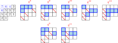
Figure 9. The excited diagrams $D$ for $(4^{3}2/31)$, their respective excited-arrays $A_{D}$ (the broken diagonals correspond to the $1$s in $A_{D}$) and weights $q^{\omega(A_{D})}=q^{a(D)}$ where $\omega(A_{D})$ is the sum of hook-lengths of the support of $A_{D}$ and $a(D)=\sum_{u\in\overline{D}}(\lambda^{\prime}_{j}-i)$.

Since by Theorem 1.5 we understand the image of the Hillman–Grassl map on SSYT of skew shape then we are able to give a generalization of the trace generating function (1.7) for these SSYT.

Proof of Theorem 1.8.

By Theorem 7.7 a tableau $T$ has shape $\lambda/\mu$ if and only if $A:=\Phi(T)$ is in $\mathcal{A}_{D}^{*}$ for some excited diagram $D\in\mathcal{E}(\lambda/\mu)$. Thus,

(7.2) $$\sum_{T\in\operatorname{SSYT}(\lambda/\mu)}\hskip 1.70709ptq^{|T|}\hskip 0.85355ptt^{\mathrm{tr}(T)}\,=\,\sum_{D\in\mathcal{E}(\lambda/\mu)}\,\sum_{T\in\Phi^{-1}(\mathcal{A}_{D}^{*})}\hskip 1.70709ptq^{|T|}\hskip 0.85355ptt^{\mathrm{tr}(T)}\,,$$

where for each $D\in\mathcal{E}(\lambda/\mu)$ we have:

(7.3) $$\sum_{T\in\Phi^{-1}(\mathcal{A}_{D}^{*})}\hskip 1.70709ptq^{|T|}\,=\,q^{\omega(A_{D})}\hskip 1.70709pt\prod_{u\in\overline{D}}\hskip 1.70709pt\frac{1}{1-q^{h(u)}}\,.$$

Next, by Proposition 5.5 for $k=0$, the trace $\mathrm{tr}(\pi)$ equals $|A_{0}|$, the sum of the entries of $A$ in the Durfee square $\square^{\lambda}$ of $\lambda$. Therefore, we refine (7.3) to keep track of the trace of the SSYT and obtain

(7.4) $$\sum_{T\in\Phi^{-1}(\mathcal{A}_{D}^{*})}\hskip 1.70709ptq^{|T|}\hskip 0.85355ptt^{\mathrm{tr}(T)}\,=\,q^{\omega(A_{D})}\hskip 0.85355ptt^{c(D)}\,\prod_{u\in\overline{D}\cap\square^{\lambda}}\frac{1}{1-t\hskip 0.85355ptq^{h(u)}}\,\prod_{u\in\overline{D}\setminus\square^{\lambda}}\frac{1}{1-q^{h(u)}},$$

where $c(D)=|\mathsf{supp}(A_{D})\cap\square^{\lambda}|$ and $\omega(A_{D})=a(D)$. Combining (7.2) and (7.4) gives the result. ∎

Proof of Theorem 7.7: First we use Theorem 6.3 to show that $\Phi^{-1}(\bigcup_{U\in\mathcal{E}(\lambda/\mu)}\mathcal{A}^{*}_{D})$ consists of RPP of skew shape $\lambda/\mu$ (Lemma 7.10). Then we show that these RPP are also column-strict (Lemma 7.11). These two results and the fact that $\Phi^{-1}$ is injective imply that

$$\Phi^{-1}:\bigcup_{U\in\mathcal{E}(\lambda/\mu)}\mathcal{A}^{*}_{D}\hookrightarrow\operatorname{SSYT}(\lambda/\mu)\hskip 1.70709pt.$$

In addition, since $\Phi$ is weight preserving, we have:

(7.5) $$s_{\lambda/\mu}(1,q,q^{2},\ldots)-F(q)\in\mathbb{N}[[q]]\hskip 1.70709pt,$$

where

$$F(q)\,:=\,\sum_{D\in\mathcal{E}(\lambda/\mu)}q^{\omega(A_{D})}\prod_{u\in[\lambda]\setminus D}\frac{1}{1-q^{h(u)}}\,.$$

By Theorem 1.4 and the equality $a(D)=\omega(A_{D})$ (Proposition 7.16), it follows that the difference in (7.5) is zero. Therefore, the restricted map $\Phi$ is a bijection between tableaux in $\operatorname{SSYT}(\lambda/\mu)$ and arrays in $\bigcup_{U\in\mathcal{E}(\lambda/\mu)}\mathcal{A}^{*}_{D}$, as desired. ∎

7.2. $\Phi^{-1}(\mathcal{A}^{*}_{D})$ are RPP of skew shape

Given an excited diagram $D\in\mathcal{E}(\lambda/\mu)$, let $\mathcal{A}_{D}$ be the set of arrays of nonnegative integers of shape $\lambda$ with support in $[\lambda]\setminus D$. Note that the set of excited arrays $\mathcal{A}^{*}_{D}$ from Definition 7.6 is contained in $\mathcal{A}_{D}$. We show that the RPP in $\Phi^{-1}(\mathcal{A}_{D})$ have support contained in $\lambda/\mu$ and therefore so do the RPP in $\Phi^{-1}(\mathcal{A}^{*}_{D})$.

Lemma 7.10.

For each excited diagram $D\in\mathcal{E}(\lambda/\mu)$, the reverse plane partitions in $\Phi^{-1}(\mathcal{A}^{*}_{D})$ have support contained in $\lambda/\mu$.

Proof.

By Lemma 6.7, the support of arrays in $\mathcal{A}_{D}$ are pleasant diagrams in $\mathcal{P}(\lambda/\mu)$. So by Theorem 6.3 it follows that $\Phi^{-1}(\mathcal{A}_{D})\subseteq\operatorname{RPP}(\lambda/\mu)$. Since $\mathcal{A}^{*}_{D}\subseteq\mathcal{A}_{D}$, the result follows. ∎

7.3. $\Phi^{-1}(\mathcal{A}^{*}_{D})$ are column strict skew RPP

Lemma 7.11.

For each excited diagram $D\in\mathcal{E}(\lambda/\mu)$, the reverse plane partitions in $\Phi^{-1}(\mathcal{A}^{*}_{D})$ are column strict skew RPPs of shape $\lambda/\mu$.

Let $\pi$ be the reverse plane partition $\Phi^{-1}(A)$ for $A\in\mathcal{A}^{*}_{D}$ and $D\in\mathcal{E}(\lambda/\mu)$. By Lemma 7.10, we know that $\pi$ has support in the skew shape $\lambda/\mu$. We show that $\pi$ has strictly increasing columns by comparing any two adjacent entries from the same column of $\pi$ . Consider the two adjacent diagonals of $\pi$ to which the corresponding entries belong and let $\nu^{1}$ and $\nu^{2}$ be the partitions obtained by reading these diagonals bottom to top. There are two cases depending on whether the diagonals end in the same column or in the same row of $\lambda/\mu$;

• If the diagonals end in the same column, then it suffices to show that $\nu^{2}_{i}<\nu^{1}_{i}$ for all $i$.

• If the diagonals end in the same row, then it suffices to show that $\nu^{2}_{i+1}<\nu^{1}_{i}$ for all $i$.

Before we treat these cases we prove the following Lemma needed for both.

Lemma 7.12.

Let $M$ be a rectangular array coming from $A\in\mathcal{A}^{*}_{D}$ with NW corner $(1,1)$. Then the first column of $P=I(\Psi({M}^{\updownarrow}))$ is  $(1,\ldots,h)$, where $h$ is the height of $P$.

Proof.

We will use the symmetry of the RSK correspondence. Recall that $\Psi(N)=(P,Q)$ for some rectangular array $N$ then $\Psi(N^{T})=(Q,P)$ so that $P$ is the recording tableaux by doing the RSK on $N$ row by row, bottom to top. Thus the first column of $P$ gives the row numbers of $N$ where the height of the insertion tableaux increased by one.

Let $R$ be the rectangular shape of $M$. By Greene’s theorem, $h$ is equal to the length of the longest decreasing subsequence in $M$. By Lemma 6.7, $h$ is at most the length of longest diagonal of $R/\mu$.

Note that $M$ contains a broken diagonal of length at least $h-1$ since either the longest diagonal of length $h$ in $R/\mu$ ends in a vertical step of $\mu$, in which case $M$ has a broken diagonal of the same length, or the longest diagonal ends in a horizontal step of $\mu$ in which case $M$ has a broken diagonal of length $h-1$.

Let $\mathsf{d}$ be such a broken diagonal. Since a broken diagonal is a decreasing subsequence that spans consecutive rows, then $\mathsf{d}$ spans the lower $h-1$ rows of $M$. This guarantees that the first column of $P$ is $1,2,\ldots,h-1,c$, where $c\geq h$ is the row where we first get a decreasing subsequence of length $h$.

Assume there is a longest decreasing subsequence $\mathfrak{d}$ of length $h$ whose first cell $x=(i_{1},j_{1})$ is in a row $c=i_{1}>h$ (counting rows bottom to top), and take both $i_{1}$ and $j_{1}$ to be minimal.

Either $x$ is inside or outside of $[\mu]$. If $x$ is outside then there is a diagonal that ends in row $i_{1}-1$ to the left of $x$, which results in a broken diagonal of length $i_{1}-1\geq h$ in the excited diagram. Hence, there is a decreasing subsequence of length $h$ starting at a lower row than the row $i_{1}$ of $x$, leading to a contradiction. See Figure 10 : Left.

When $x$ is inside of $[\mu]$ then there is an excited cell below $x$ in the same diagonal. There must be a broken diagonal $\mathsf{d}^{\prime}$ that reaches at least row $i_{1}-1$ below or to the left of $x$. At row $i_{1}$, the sequence $\mathfrak{d}$ is above $\mathsf{d}^{\prime}$ and the last entry of $\mathfrak{d}$ is below $\mathsf{d}^{\prime}$, as otherwise $\mathfrak{d}$ would be shorter than $\mathsf{d}^{\prime}$. Thus the sequence $\mathfrak{d}$ and the broken diagonal $\mathsf{d}^{\prime}$ cross. Consider the first crossing tracing top down. Let $a$ be the last cell of $\mathfrak{d}$ before this crossing and let $b$ be the cell of $\mathfrak{d}$ on or after the crossing. Note that below $a$ in the same column there is either a nonzero from $\mathsf{d}^{\prime}$ or a zero from the excited horizontal segment of $\mathsf{d}^{\prime}$. In either case, $a$ is higher than the lowest cell of $\mathsf{d}^{\prime}$ to the left of $b$. Define $\mathfrak{d}^{\prime}$ to be the sequence consisting of the segment of $\mathsf{d}^{\prime}$ from row $i_{1}-1$ up until the crossing followed by the segment of $\mathfrak{d}$ from cell $b$ onwards (see Figure 10: Right). Note that $\mathfrak{d}^{\prime}$ is a decreasing sequence of $R$ that starts at row $i_{1}-1$ and column $\leq j_{1}$ and has length $h$ since $\mathfrak{d}$ includes a nonzero element from the row below the row $a$. This contradicts the minimality of $x$.

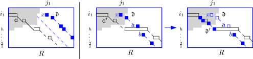
Figure 10. Two cases to consider in the proof of Lemma 7.12 depending on whether cell $x=(i_{1},j_{1})$ is outside or inside of $[\mu]$.

In summary, we conclude that $c=h$, and the first column of $P$ is $(1,\ldots,h)$, as desired. This finishes the proof. ∎

Column strictness in Case 1.  By Corollary 5.8 we have $\nu^{1}=\mathrm{shape}(P^{1})$ and $\nu^{2}=\mathrm{shape}(P^{2})$ where $P^{1}=I(\Psi(M^{1}))$, $P^{2}=I(\Psi(M^{2}))$, and the rectangular array $M^{1}={A_{t}}^{\leftrightarrow}$ is obtained from the rectangular array $M^{2}={A_{t+1}}^{\leftrightarrow}$ by adding a row $w$ at the end. Thus $\nu^{1}$ is the shape of the insertion tableau obtained by row inserting $w$ (from left to right) in the insertion tableau $I(\Psi(M^{2}))$ of shape $\nu^{2}$.

Proposition 7.13.

In Case 1 we have $\nu^{2}_{i}<\nu^{1}_{i}$ for $1\leq i\leq\min\{\ell(\nu^{1}),\ell(\nu^{2})\}$.

Proof.

Let $P=I(\Psi(M^{1}))$ and $Q=R(\Psi(M^{1}))$ (in this case, $M^{1}$ is being read top to bottom, left to right, i.e. row by row starting from the right, from the original array $A_{t}$ before the flip). Let $m$ be the height of $M^{1}$. The strict inequality is equivalent to the fact that the insertion of the last row in $P$ results in an extension of every row, i.e. every row of the recording tableau $Q$ has at least one entry equal to $m$. We will prove the last statement. Note that by the symmetry of the RSK correspondence, we have $Q$ is the insertion tableaux for $A_{t}$ when read column by column from right to left.

Claim:  Let $h$ be the height of $Q$, i.e. the longest decreasing subsequence of $M^{1}$. Then row $i$ of $Q$ contains at least one entry from each of $m,\ldots,m-h+i$.

Note that $h$ is equal to the length of the longest broken diagonal or one more than that. We prove the claim by induction on the number of columns in $M^{1}$, i.e. in $A_{t}$. Let $M^{1}=[u^{1},u^{2},\ldots,u^{r}]$, where $u^{i}$ is its $i$-th column. In terms of the excited array $A_{t}$, we have that $u^{r}$ is the first column of $A_{t}$ and $u^{1}$ – the last. Suppose that the claim is true for $A_{t}$ restricted to its first $r-1$ columns, which is still an excited array by definition, and let $u=u^{1}$ be its last column. Let $Q$ be the insertion tableaux of $[u^{2},\ldots,u^{r}]$ read column by column, i.e. $Q=u^{2}\leftarrow u^{3}\leftarrow\cdots$, where $\leftarrow$ indicates the insertion of the corresponding sequence. Then let $Q^{\prime}$ be the insertion tableaux corresponding to $A_{t}$, so $Q^{\prime}=u\leftarrow\mathrm{reading}(Q)$ by Knuth equivalence. The reading word is obtained from $Q$ by reading it row by row from the bottom to the top, each row read left to right.

First, suppose that $u$ does not increase the length of the longest decreasing subsequence, so $Q^{\prime}$ has also height $h$. Let $a\in[m-j+i,m]$ be a number present in row $i$ of $Q$. When it is inserted in $Q^{\prime}$ it will first be added to row 1, where there could be other entries equal to $a$ already present. The first such entry $a$ will be bumped by something $\leq a-1$ coming from inserting row $i-1$ of $Q$ into $Q^{\prime}$. This had to happen in $Q$ since $a$ reached row $i$. From then on the same numbers will bump each other as in the original insertion which created $Q$. Thus an entry equal to $a$ will reach row $i$ after the $i-1$ bumps. Since the height of $Q^{\prime}$ is unchanged, the claim holds as it pertains only to the original entries $a$ from $Q$ which again occupy the corresponding rows.

Next, suppose that $u$ increases the length of the longest decreasing subsequence to $h+1$. Then the longest broken diagonal in $A_{t}$ has length at least $h$. Also, column $u$ must have an element equal to $m$, i.e. a nonzero entry in $A_{t}$’s lower right corner. Moreover, we claim that the longest decreasing subsequence has to occupy the consecutive rows of $A_{t}$ from $m-h$ to $m$, and thus the longest decreasing subsequences in $u,\mathrm{reading}(Q)$ are $m,m-1,\ldots,m-h$. This is shown within the proof of Lemma 7.12. From there on, in $u\leftarrow\mathrm{reading}(Q)$ we have element $m$ from $u$ bumped by something $\leq m-1$ from the last row of $Q$. Afterwards, the bumps happen similarly to the previous case and the numbers from $Q$ reach their corresponding rows, so the $m$ from $u$ reaches eventually one row below, i.e. row $h+1$. The entry $m-h$ from the longest decreasing sequence is inserted from the first row of $Q$ and is, therefore, in row 1 of $Q^{\prime}$, so by iteration $Q^{\prime}$ has the desired structure. This ends the proof of the claim and thus the Proposition. ∎

Column strictness in Case 2.  By Corollary 5.8 we have $\nu^{1}=\mathrm{shape}(P^{1})$ where $P^{1}=I(\Psi({M^{1}}))$ and $\nu^{2}=\mathrm{shape}(P^{2})$ where $P^{2}=I(\Psi({M^{2}}))$ and the rectangular array $M^{2}={A_{t+1}}^{\updownarrow}$ is obtained from the rectangular array $M^{1}={A_{t}}^{\updownarrow}$ by adding a column $v$ at the end (we read column by column SW to NE). Thus $\nu^{2}$ is the shape of the insertion tableau obtained by row inserting $v$ (from top to bottom) in the insertion tableau $I(\Psi(M^{1}))$ of shape $\nu^{1}$.

Proposition 7.14.

For Case 2 we have $\nu^{2}_{i+1}<\nu^{1}_{i}$ for $1\leq i\leq\min\{\ell(\nu^{1}),\ell(\nu^{2})-1\}$.

We prove a stronger statement that requires some notation. Let $P$ be the insertion tableau of shape $\nu$ where $M={B}^{\updownarrow}$ for some rectangular array $B$ of $A\in\mathcal{A}^{*}_{D}$ with NW corner $(1,1)$. for a positive integer $k$, let $P_{i}(k)$ be the number of entries in row $i$ of $P$ which are $\leq k$.

Lemma 7.15.

With $P$ and $P_{i}(k)$ as defined above, for $k>1$ we have

• If $P_{i}(k)>0$ then $P_{i}(k)<P_{i-1}(k-1)$,

• If $k$ is in row $i$ of $P$ where $k>i$ then $P_{i}(k-1)>0$.

Proof of Proposition 7.14.

We first show that Lemma 7.15 implies that the insertion path of the RSK map of $M$ moves strictly to the left. To see this, let $P$ be the resulting tableaux obtained at some stage of the insertion when $j$ is inserted in row $1$ and bumps $j_{1}>j$ to row $2$. Then $j$ is inserted at position $P_{1}(j_{1}-1)$ in row 1 and $j_{1}$ is inserted at position $P_{2}(j_{1})>0$ in row 2. By Condition (i), $P_{2}(j_{1})<P_{1}(j_{1}-1)$. Iterating this argument as elements get bumped in lower rows implies the claim.

Next, note that a bumped element at position $\nu^{1}_{2}+1$ from row 1 of $P^{1}$ cannot be added to row 2 as otherwise the insertion path would move strictly down, violating Condition (i). Thus the only elements from row 1 of $P^{1}$ that can be added to row 2 in $P^{2}$ are those in positions $>\nu^{1}_{2}+1$. And so there are no more than $\nu^{1}_{1}-\nu^{1}_{2}-1$ such elements implying that $\nu^{2}_{2}\leq\nu^{1}_{1}-1$. Iterating this argument in the other rows implies the result. ∎

Proof of Lemma 7.15.

Note that Condition (ii) for $k=i+1$ follows by Lemma 7.12. Note that the statement of the lemma holds for any step of the insertion, since it applies for $P$ as a recording tableaux. Since $P_{i}(k)$ are increasing for $k$ with $i$ fixed then Condition (ii) holds. We claim that after each single insertion of $\Psi$, Condition (i) still holds. We prove this when inserting an element $j$ in row $r$. Iterating this argument as elements get bumped in lower rows implies the claim.

Assume $P$ verifies Condition (i) and we insert $j$ in row $r$ of $P$ to obtain a tableaux $P^{\prime}$ of shape $\nu^{\prime}$. By Lemma 7.12 we have $j\geq r$. If $j$ is added to the end of the row then Condition (i) still holds for $P^{\prime}$ since $P^{\prime}_{r}(j)>P_{r}(j)$. If $j$ bumps $j_{1}$ in row $r$ then $j_{1}>j$ and

(7.6) $$P^{\prime}_{r}(j)\hskip 1.70709pt=\hskip 1.70709ptP^{\prime}_{r}(j_{1}-1)=P_{r}(j_{1}-1)+1\hskip 1.70709pt,\qquad P^{\prime}_{r}(j_{1})\hskip 1.70709pt=\hskip 1.70709ptP_{r}(j_{1})$$

and all other $P^{\prime}_{r}(i)=P_{r}(i)$ remain the same.

Next, we insert $j_{1}$ in row $r+1$ of $P$. Regardless of whether $j_{1}$ is added to the end of the row or bumps another element to row $r+2$, we have

$$P^{\prime}_{r+1}(j)\hskip 1.70709pt=\hskip 1.70709ptP_{r+1}(j)\hskip 1.70709pt,\qquad P^{\prime}_{r+1}(j_{1})\hskip 1.70709pt=\hskip 1.70709ptP_{r+1}(j_{1})+1\hskip 1.70709pt,$$

and all other $P^{\prime}_{r+1}(i)=P_{r+1}(i)$ remain the same. Since $P^{\prime}_{r}(b)\geq P_{r}(b)$ for all $b$, we need to verify Condition (i) only when $P^{\prime}_{r+1}$ increased with respect to $P_{r+1}$.

By Lemma 7.12, we have either row $r+1$ of $P$ is nonempty and thus $P_{r+1}(j_{1})>0$, or else we must have $j_{1}=r+1$. In the first case Condition (i) applies to $P$ and we have $P_{r+1}(j_{1})<P_{r}(j_{1}-1)$. By (7.6), we have

$$P^{\prime}_{r+1}(j_{1})=P_{r+1}(j_{1})+1<P_{r}(j_{1}-1)+1=P^{\prime}_{r}(j_{1}-1).$$

Finally, suppose $j_{1}=r+1$. Since $j\geq r$, we then have $j=r$, and $r$ must have been present in row $r$ in $P$ by Lemma 7.12. Thus $P_{r}(r)\geq 1$ and

$$P^{\prime}_{r}(r)\hskip 1.70709pt\geq\hskip 1.70709pt2\hskip 1.70709pt>\hskip 1.70709ptP^{\prime}_{r+1}\hskip 1.70709pt=\hskip 1.70709pt1\hskip 1.70709pt.$$

Therefore, Condition (i) is verified for rows $r$ and $r+1$ of $P^{\prime}$, as desired. ∎

7.4. Equality between $a(D)$ and $\omega(A_{D})$

Proposition 7.16.

For all excited diagrams $D\in\mathcal{E}(\lambda/\mu)$, $a(D)=\sum_{(i,j)\in\overline{D}}(\lambda^{\prime}_{j}-i)$ equals $\omega(A_{D})$.

First, we show that for the Young diagram of $\mu$ both statistics $a(\cdot)$ and $\omega(\cdot)$ agree.

Lemma 7.17.

For a Young diagram $[\mu]\in\mathcal{E}(\lambda/\mu)$ we have $a([\mu])=\omega(A_{\mu})$.

Proof.

We proceed by induction on $|\mu|$ with $\lambda$ fixed. When $\mu=\varnothing$ we have both

$$a(D_{\varnothing})\,=\,\sum_{(i,j)\in\lambda}(\lambda^{\prime}_{j}-i)\,=\,\sum_{i}\binom{\lambda^{\prime}_{i}}{2}=\sum_{i}(i-1)\lambda_{i}=b(\lambda)\hskip 1.70709pt.$$

Now, either directly or by Remark 7.5 for $\mu=\varnothing$,

$$\omega(A_{\varnothing})=\sum_{(i,j)\in\lambda,i>j}h(i,j)=b(\lambda).$$

Let $\nu$ be obtained from $\mu$ by adding a cell at position $(a,b)$. Then

$$a([\mu])-a(D_{\nu})\hskip 1.70709pt=\hskip 1.70709pt\lambda^{\prime}_{b}-a\hskip 0.85355pt.$$

Next, the array $A_{\nu}$ is obtained from $A_{\mu}$ by moving the ones in diagonal $\mathsf{d}_{b}=\{(i,j)\mid i-j=\mu_{b}-b\}$ to diagonal $\mathsf{d}^{\prime}_{b}=\{(i,j)\mid i-j=\mu_{b}+1-b\}$ and leaving the rest unchanged. Thus

(7.7) $$\omega(A_{\mu})-\omega(A_{\nu})\hskip 1.70709pt=\hskip 1.70709pt\sum_{u\in\mathsf{d}_{b}}h(u)-\sum_{u\in\mathsf{d}^{\prime}_{b}}h(u)\hskip 0.85355pt.$$

Since $h(i,j)=\lambda_{i}+\lambda^{\prime}_{j}-i-j+1$, then $h(i,j)-h(i,j+1)$ cancels $\lambda_{i}-i+1$ and $h(i,j)-h(i+1,j)$ cancels the terms $\lambda^{\prime}_{j}-j$. So by doing horizontal and vertical cancellations on diagonals $\mathsf{d}_{k}$ and $\mathsf{d}^{\prime}_{k}$ in (7.7) (see Figure 11, Left) we conclude that either

$$\sum_{u\in\mathsf{d}_{b}}h(u)-\sum_{u\in\mathsf{d}^{\prime}_{b}}h(u)=\lambda^{\prime}_{b}-b-(\lambda^{\prime}_{c}-c)$$

if the diagonals $\mathsf{d}^{\prime}_{b}$ and $\mathsf{d}_{b}$ have the same length, or

$$\sum_{u\in\mathsf{d}_{b}}h(u)-\sum_{u\in\mathsf{d}^{\prime}_{b}}h(u)=\lambda^{\prime}_{b}-b+(\lambda_{r}-r+1).$$

otherwise. In both these cases $\lambda^{\prime}_{c}-c+b$ and $r-\lambda_{r}+b-1$ are equal to $a$. Thus,

$$\omega(A_{\mu})-\omega(A_{\nu})=\lambda^{\prime}_{b}-a=a([\mu])-a(D_{\nu}).$$

Then by induction it follows that $\omega(A_{\nu})=a(D_{\nu})$. ∎

Lemma 7.18.

Let $D^{\prime}\in\mathcal{E}(\lambda/\mu)$ be obtained from $D\in\mathcal{E}(\lambda/\mu)$ with one excited move. Then $a(D^{\prime})-a(D)=\omega(A_{D^{\prime}})-\omega(A_{D})$.

Proof.

Suppose $D^{\prime}$ is obtained from $D$ by replacing $(i,j)$ by $(i+1,j+1)$ then

$$a(D^{\prime})-a(D)=\lambda^{\prime}_{j}-i-(\lambda^{\prime}_{j+1}-i-1)=\lambda^{\prime}_{j}-\lambda^{\prime}_{j+1}+1,$$

and since $h_{(s,t)}=\lambda_{s}-s+\lambda^{\prime}_{t}-t+1$ then

$$\omega(A_{D^{\prime}})-\omega(A_{D})=h_{(i+1,j)}-h_{(i+1,j+1)}=\lambda^{\prime}_{j}-\lambda^{\prime}_{j+1}+1.$$

We illustrate these differences in Figure 11: Right. ∎

Figure 11. The equality of statistics $a(D)$ and $\omega(A_{D})$.

8. Skew SSYT with bounded parts

Here we consider the generating function of skew SSYT with entries in $[M]$. The analogous question for straight-shape SSYTs is answered by Stanley’s elegant hook-content formula [S3, §7.21].

Theorem 8.1 (hook-content formula [S1]).

$$s_{\lambda}(1,q,q^{2},\ldots,q^{M-1})=q^{b(\lambda)}\prod_{u\in[\lambda]}\frac{1-q^{M+c(u)}}{1-q^{h(u)}},$$

where $c(u)=j-i$ is the content of the square $u=(i,j)$.

In this section we discuss whether there is a hook-content formula for skew shapes in terms of excited diagrams. We are able to write such formulas for border strips but our approach does not extend to general shapes. We start by considering the case of the inverted hook $\lambda/\mu=k^{d}/(k-1)^{d-1}$, then we look at the case of border strips and we end by briefly discussing the case of general skew shapes.

8.1. Inverted hooks

We start studying the border strip $\lambda/\mu=(k^{d})/(k-1)^{d-1}$; an inverted hook. From Example 3.2 the complements of excited diagrams of this shape correspond to lattice paths $\gamma$ from $(d,1)$ to $(1,k)$.

Proposition 8.2.

(8.1) $$s_{\lambda/\mu}(1,q,\ldots,q^{M-1})\,=\,\sum_{\gamma:(d,1)\to(1,k)}q^{a(\gamma)}\cdot h_{M-d+1}(1,q^{h(u_{1})},q^{h(u_{2})},\ldots,q^{h(u_{k+d-1})})\hskip 0.85355pt,$$

where $u_{1},u_{2},\ldots,u_{k+d-1}$ are the cells in the path $\gamma$.

Proof.

By Theorem 7.7, the image of a SSYT $T$ of this shape via Hillman–Grassl is an array $A$ with support on a lattice path $\gamma:(d,1)\to(1,k)$ (i.e. the complement o an excited diagram) with certain forced nonzero entries. These nonzero entries are exactly on cells of vertical steps, including outer corners but not inner corners and excluding $(1,k)$ (see Example 8.3).

The maximal entry in $A$ is in the cell $(d,1)$ and the maximal entry in $T$ is in the cell $(d,k)$. We claim that the latter entry is the sum of all the entries in the initial array. To see this note that in the steps of the inverse Hillman–Grassl map $A\mapsto T$, every strip of $1$s added to the RPP of support in $\lambda/\mu$ starts from a cell in row $d$ and passes through cell $(d,k)$.

Let $\gamma=(u_{1},\ldots,u_{k+d-1})$ be a lattice path from $(d,1)$ to $(1,k)$ along the squares with (top) corners at positions $(\gamma^{1}_{i},\gamma^{2}_{i})$, so that the cells of the path are $u_{1}=(d,1),u_{2}=(d-1,1)\ldots(\gamma^{1}_{1},\gamma^{1}_{1})(\gamma^{1}_{1}+1,\gamma^{2}_{1})\ldots(\gamma^{1}_{2},\gamma^{2}_{1})\ldots...$. The designated nonzero cells on $\gamma$ are the ones located below these corners: $(d,1)\ldots(\gamma^{1}_{1}-1,1)$ etc. We notice that we have exactly $d-1$ such entries. If the values in $A$ of the entries in the path are $\alpha_{1},\ldots,\alpha_{k+d-1}$, the maximal entry in $T$ will be $\alpha_{1}+\cdots+\alpha_{k+d-1}$. The total weight of the resulting SSYT is then $\prod_{u_{i}\in\gamma}q^{h(u_{i})\alpha_{i}}$. The total contribution of the path $\gamma$ over all possible such values $\alpha$ is then

$$\sum_{\alpha_{1}+\cdots+\alpha_{k+d-1}\leq M}\prod_{u_{i}\in\gamma}q^{h(u_{i})\alpha_{i}}\, =\,\left(\prod_{u\in\gamma,\text{ nonzero}}q^{h(u)}\right)\times h_{M-d+1}(1,q^{h(u_{1})},q^{h(u_{2})},\ldots,q^{h(u_{k+d-1})})$$

$$=\,q^{a(\gamma)}\cdot h_{M-d+1}(1,q^{h(u_{1})},q^{h(u_{2})},\ldots,q^{h(u_{k+d-1})})\hskip 0.85355pt,$$

as desired. ∎

Example 8.3.

For the reverse hook shape $(3^{3}/2^{2})$, the six paths (complements of excited diagrams) with their corresponding nonzero entries of the arrays are the following:

.

Thus, in this case (8.1) gives

$$s_{3^{3}/2^{2}}(1,q,\ldots,q^{M-1})\,=\,q^{3}h_{M-2}(1,q^{3},q^{2},q^{1},q^{2},q^{3})\hskip 1.70709pt+\hskip 1.70709pt\cdots\hskip 1.70709pt+\hskip 1.70709ptq^{7}h_{M-2}(1,q^{3},q^{4},q^{5},q^{4},q^{3})\hskip 0.85355pt.$$

Note that in contrast with the principal specialization of $h_{k}$, the specializations in (8.1) do not necessarily have nice product formulas. For instance, when $M=3$ the first term in the RHS above gives

$$h_{1}(1,q^{3},q^{2},q^{1},q^{2},q^{3})\hskip 1.70709pt=\hskip 1.70709pt1+q^{1}+2q^{2}+2q^{3}\hskip 1.70709pt=\hskip 1.70709pt(q+1)(2q^{2}+1)\hskip 0.85355pt.$$

Remark 8.4.

When we evaluate $q=1$ in (8.1), the hook lengths involved in the evaluation of the complete symmetric function become $1$ and so each path $\gamma$ contributes $h_{M-b+1}(1^{a+b})=\binom{M+a}{a+b-1}$. Summing this equal contribution over all paths gives

$$s_{\lambda/\mu}(1^{M})\,=\,\sum_{\gamma:(d,1)\to(1,k)}\binom{M+k}{k+d-1}\,=\,\binom{k+d-2}{k-1}\binom{M+k}{k+d-1}\hskip 0.85355pt.$$

Since $s_{\lambda/\mu}=s_{k1^{d-1}}$, this is precisely what the hook-content formula gives for $s_{k1^{d-1}}(1^{M})$.

8.2. Border strips

A border strip is a (connected) skew shape $\lambda/\mu$ containing no $2\times 2$ box. The inverted hook is an example of a border strip. Similarly to inverted hooks, complements of excited diagrams of border strips correspond to lattice paths $\gamma$ from $(\lambda^{\prime}_{1},1)$ to $(1,\lambda_{1})$ that stay inside $\lambda$.

To state the result, we nee some notation. Let $\lambda/\mu$ be a border strip with corners (these time we consider the outer corners of $\lambda$) at positions $(x_{i},y_{i})$ (starting from the bottom left) and divide the diagram $\lambda$ with the lines $x=x_{i}$ and $y=y_{j}$ into rectangular regions $R_{ij}$. A lattice path $\gamma:(\lambda^{\prime}_{1},1)\to(1,\lambda_{1})$ inside $\lambda$ may intersect some of these rectangles. Let $\gamma=\gamma^{1},\gamma^{2},\ldots$ be the subpaths of $\gamma$, where each $\gamma^{\ell}$ belongs to a unique rectangle $R_{i_{\ell}j_{\ell}}$. We denote by $g^{\ell}$ a sequence of nonnegative integers in the cells of $\gamma^{\ell}$, and by $|g^{\ell}|$ the sum of these entries.

Proposition 8.5.

For a border strip $\lambda/\mu$ we have that

(8.2) $$s_{\lambda/\mu}(1,q,\ldots,q^{M-1})=\sum_{\gamma:(\lambda^{\prime}_{1},1)\to(1,\lambda_{1}),\gamma\subseteq[\lambda]}q^{a(\gamma)}\sum_{g^{1},g^{2},\ldots:\\ \sum_{\ell:i_{\ell}\geq i,j_{\ell}\leq i}|g^{\ell}|+b_{\ell}\leq M}q^{\sum_{u\in\gamma}g_{u}h(u)}.$$

Proof.

Let $T$ be a SSYT of shape $\lambda/\mu$ with entries $\leq M$ and $A=\Phi(T)$. By Theorem 7.7, the support of $A$ is on a path $\gamma:(\lambda^{\prime}_{1},1)\to(1,\lambda_{1})$ inside of $\lambda$.

By the analogue of Greene’s theorem for $\Phi$ (Theorem 5.6 (i)), the maximal entry in $T$ in each rectangle is the sum of the entries in $A$ within that rectangle, since the nonzero entries lie on $\gamma$ and so form a single increasing sequence. Moreover, the forced nonzero entries are on the vertical steps of $\gamma$. As in the case of inverted hooks, the bound $M$ is again involved in the total sum over the path segments in each rectangle. However, in a border strip the rectangles overlap, and so would the sums over the path elements.

We divide $\gamma=\gamma^{1},\gamma^{2},\ldots$ into subpaths, where each $\gamma^{\ell}$ belongs to a unique rectangle $R_{i_{\ell}j_{\ell}}$. We must have that by monotonicity of $\gamma$ $i_{1}\leq i_{2}\leq\cdots$ and $j_{1}\leq j_{2}\leq\cdots$, and by connectivity of $\gamma$ that $i_{\ell}\geq i_{\ell+1}-1$ and $j_{\ell}\geq j_{\ell+1}-1$. The entries in $A$ along $\gamma^{\ell}$ are the sequence $g^{\ell}$, with sum $M_{\ell}+b_{\ell}$, for some $M_{\ell}$. By the properties of the Hilman–Grassl bijection, we need to have forced nonzero elements on the vertical steps of $\gamma$. We can subtract $1$ from them and consider nonnegative elements summing up to $M_{\ell}$. Again by the properties of the bijection, each rectangle $R_{ii}$ in $A$ has to contain a longest increasing subsequence of total sum at most $M$ in order to have the entry in the corner of $T$ to be at most $M$. In this case there is only one longest increasing subsequence in $A$, which is the path $\gamma$ itself. Thus, we have

$$\sum_{\ell:\hskip 1.70709pti_{\ell}\geq i\geq j_{\ell}}\hskip 1.70709pt(M_{\ell}+b_{\ell})\,\leq\,M.$$

We conclude:

$$s_{\lambda/\mu}(1,q,\ldots,q^{M-1})\,=\,\sum_{\gamma}\hskip 1.70709ptq^{\sum_{u\in\gamma,\text{ vertical step }}h(u)}\,\hskip 1.70709pt\sum\hskip 1.70709ptq^{\sum_{u\in\gamma}\hskip 0.85355ptg_{u}\hskip 0.85355pth(u)}\hskip 0.85355pt,$$

where the last sum is over all  $g^{1},g^{2},\ldots$  s.t. $\sum_{\ell:\hskip 1.70709pti_{\ell}\geq i\geq j_{\ell}}|g^{\ell}|+b_{\ell}\hskip 1.70709pt\leq\hskip 1.70709ptM$. Now observe that the sum of the hooks of the forced nonzero entries in $\gamma$ is $a(\gamma)$, which implies the result. ∎

Remark 8.6.

The sums over the sequences $g^{i}$ in formula (8.2) cannot be simplified any further, since the restrictions are not over independent pieces. However, one can think of the inequalities as a simple linear program with coefficients 0 or 1, and the entries in the sequence $g^{1},\ldots,g^{\ell}$ as integral points in a polytope defined by these inequalities.

Corollary 8.7.

$$s_{\lambda/\mu}(1^{M})\,=\,\sum_{\gamma}\sum_{M_{1},\ldots:\hskip 1.70709pt\sum_{\ell:i_{\ell}\geq i\geq j_{\ell}}M_{\ell}+b_{\ell}\leq M}\hskip 1.70709pt\prod_{\ell}\binom{M_{\ell}+a_{\ell}+b_{\ell}-2}{M_{\ell}}\hskip 0.85355pt.$$

Proof.

We evaluate $q=1$ in (8.2). If the sum of entries in $g^{\ell}$ is $M_{\ell}$, and the path $\gamma^{\ell}$ has length $a_{\ell}+b_{\ell}-1$, we have that the number of ways of choosing such entries is $\binom{M_{\ell}+a_{\ell}+b_{\ell}-2}{M_{\ell}}$, and so the result follows. ∎

8.3. General skew shapes

In the general case, complements of excited diagrams correspond to tuples of non-intersecting lattice paths (see proof of Lemma 6.6). In [MPP2] we use a non-intersecting lattice path approach to upgrade the NHLF and Theorem 1.4 from border strips to general skew shapes. However, this approach does not apply for SSYT of bounded parts. This is because Proposition 8.2 shows that the bound $M$ on the entries of a SSYT $T$ of border strip shape is encoded via Hillman–Grassl as restricted sums on an array with support on lattice path $\gamma$. Two intersecting paths with restricted sums of elements can be divided into two other intersecting paths with different total sums of elements, which may not satisfy the same restriction. In other words, the usual involution on intersections, that cancels the intersecting paths contribution from the Lindström–Gessel–Viennot determinant, cannot be applied here as we cannot restrict to the same subset of paths.

9. Other formulas for the number of standard Young tableaux

In this section we give a quick review of several competing formulas for computing $f^{\lambda/\mu}$.

9.1. The Jacobi–Trudi identity

This classical formula (see e.g. [S3, §7.16]), allowing an efficient computation of these numbers. It generalizes to all Schur functions and thus gives a natural $q$-analogue for SSYT. On the negative side, this formula is not positive, nor does it give a $q$-analogue for RPP.

9.2. The Littlewood–Richardson coefficients

Equally celebrated is the positive (subtraction-free) formula

$$f^{\lambda/\mu}\,=\,\sum_{\nu\vdash|\lambda/\mu|}\,c_{\mu,\nu}^{\lambda}\hskip 1.70709ptf^{\nu}\hskip 1.70709pt,$$

where $c_{\mu,\nu}^{\lambda}$ are the Littlewood–Richardson (LR-) coefficients. This formula has a natural $q$-analogue for SSYT, but not for RPP. When LR-coefficients are defined appropriately, this $q$-analogue does have a bijective proof by a combination of the Hillman–Grassl bijection and the jeu-de-taquin map; we omit the details (cf. [Whi]).

On the negative side, the LR-coefficients are notoriously hard to compute both theoretically and practically (see [Nara]), which makes this formula difficult to use in many applications.

9.3. The Okounkov–Olshanski formula

The following curious formula is of somewhat different nature. It is also positive, which might not be immediately obvious.

Denote by $\mathsf{RT}(\mu,\ell)$ the set of reverse semistandard tableaux $T$ of shape $\mu$, which are arrays of positive integers of shape $\mu$, weakly decreasing in the rows and strictly decreasing in the columns, and with entries between $1$ and $\ell$. The Okounkov–Olshanski formula (OOF) given in [OO] states:

(OOF) $$f^{\lambda/\mu}\,=\,\frac{|\lambda/\mu|!}{\prod_{u\in[\lambda]}h(u)}\,\sum_{T\in\mathsf{RT}(\mu,\ell(\lambda))}\,\prod_{u\in[\mu]}(\lambda_{T(u)}-c(u))\hskip 1.70709pt,$$

where $c(u)=j-i$ is the content of $u=(i,j)$. The conditions on tableaux $T$ imply that the numerators here non-negative.

Example 9.1.

For $\lambda/\mu=(2^{3}1/1^{2})$, the reverse semistandard tableaux of shape $(1^{2})$ with entries $\{1,2,3,4\}$ are

$$\young(2,1)\,,\quad\young(3,1)\,,\quad\young(3,2)\,,\quad\young(4,1)\,,\quad\young(4,2)\,,\quad\young(4,3);$$

and the contents are $c(0,0)=0$ and $c(1,0)=-1$. Thus, the Okounkov–Olshanski formula gives:

$$f^{(2^{3}1/1^{2})}\,=\,\frac{5!}{5\cdot 4\cdot 3\cdot 3\cdot 2\cdot 1\cdot 1}\bigl{(}2\cdot 3+2\cdot 3+2\cdot 3+1\cdot 3+1\cdot 3+1\cdot 3\bigr{)}\,=\hskip 1.70709pt9$$

(cf. Example 3.1). Note that the (OOF) is asymmetric. For example, for $\lambda^{\prime}/\mu^{\prime}=(43/2)$, there are two reverse tableaux of shape $(2)$ with entries $\{1,2\}$.

It is illustrative to compare the NHLF and the OOF for the shape $\lambda/(1)$ since $f^{\lambda/(1)}=f^{\lambda}$. The excited diagrams $\mathcal{E}(\lambda/(1))$ consist of single boxes of the diagonal $\mathsf{d}_{0}$ of $\lambda$, thus the NHLF gives

$$f^{\lambda/(1)}=\frac{(|\lambda|-1)!}{\prod_{u\in[\lambda]}h(u)}\,\,\left[\sum_{i}h(i,i)\right].$$

On the other hand, the reverse tableau $\mathsf{RT}((1),\ell(\lambda))$ are of the form $T=\young(i)$ for $1\leq i\leq\ell(\lambda)$. For each of these tableaux $T$ we have $\lambda_{T(1,1)}=\lambda_{i}$ and $c(1,1)=0$, thus the (OOF) gives

$$f^{\lambda/(1)}=\frac{(|\lambda|-1)!}{\prod_{u\in[\lambda]}h(u)}\,\,\left[\sum_{i=1}^{\ell(\lambda)}\lambda_{i}\right].$$

Note that in both cases $\sum_{i}h(i,i)=\sum_{i}\lambda_{i}=|\lambda|$, confirming that $f^{\lambda/(1)}=f^{\lambda}$, however the summands involved in both formulas are different in number and kind.

Chen and Stanley [CS] found a SSYT  $q$-analogue of the (OOF). Their proof is algebraic; they also give a bijective proof for shapes $\lambda/(1)$. It would be very interesting to find a bijective proof of the formula and its $q$-analogue in full generality. Note that again, there is no RPP $q$-analogue in this case. On the positive side, the sizes $|\mathsf{RT}(\mu,\ell)|$ are easy to compute as the number of bounded SSYT of the (rectangle) complement shape $\overline{\mu}$; we omit the details.

9.4. Formulas from rules for equivariant Schubert structure constants

In this section we sketch how there is a formula for $f^{\lambda/\mu}$ for every rule of equivariant Schubert structure constants, a generalization of the Littlewood–Richardson coefficients.

The equivariant Schubert structure constants $C_{\mu,\nu}^{\lambda}({\bf y}):=C_{\mu,\nu}^{\lambda}(y_{1},\ldots,y_{n})$ are polynomials in $\mathbb{Z}[y_{1},\ldots,y_{n}]$ of degree $|\mu|+|\nu|-|\lambda|$ defined by the multiplication of equivariant Schubert classes $\sigma_{\mu}$ and $\sigma_{\nu}$ in the $T$-equivariant cohomology ring $H_{T}(X)$ (see [KT, TY, Knu]). When $|\mu|+|\nu|=|\lambda|$ the degree zero polynomials $C_{\mu,\nu}^{\lambda}({\bf y})$ equal the Littlewood–Richardson coefficients $c_{\mu,\nu}^{\lambda}$.

The Kostant polynomial $[X_{w}]|_{v}=\sigma_{w}(v)$ from Section 4 for Grassmannian permutations $w\preceq v$ corresponding to partitions $\mu\subseteq\lambda\subset d\times(n-d)$ is also equal to $C_{\mu,\lambda}^{\lambda}({\bf y})$, see [Bil, §5] and [Knu].

The proof of the NHLF outlined by Naruse in [Naru] is based on the following two identities.

Lemma 9.2.

(9.1) $$(-1)^{|\lambda|}\left.C_{\lambda,\lambda}^{\lambda}({\bf y})\right|_{y_{i}=i}=\prod_{u\in[\lambda]}h(u).$$

Proof.

We use Theorem 4.1 for $\mu=\lambda\subseteq d\times(n-d)$, since the only excited diagram in $\mathcal{E}(\lambda/\lambda)$ is $[\lambda]$ then

$$(-1)^{|\lambda|}C_{\lambda,\lambda}^{\lambda}({\bf y})=\prod_{(i,j)\in[\lambda]}(y_{d+j-\lambda^{\prime}_{j}}-y_{\lambda_{i}+d-i+1}).$$

Evaluating this equation at $y_{i}=i$ gives the desired formula. ∎

Lemma 9.3 (Naruse [Naru], see also [MPP2]).

$$(-1)^{|\lambda/\mu|}\,\left.\frac{C_{\mu,\lambda}^{\lambda}({\bf y})}{C_{\lambda,\lambda}^{\lambda}({\bf y})}\,\,\right|_{y_{i}=i}\,=\,\frac{f^{\lambda/\mu}}{|\lambda/\mu|!}.$$

First, we swiftly recover the hook-length formula for $f^{\lambda}$.

Corollary 9.4.

Lemma 9.3 implies the HLF (1.1).

Proof.

By combining Lemma 9.3 for $\mu=\varnothing$, (9.1), and using $C_{\varnothing,\lambda}^{\lambda}({\bf y})=1$ we obtain the HLF. ∎

Second, we obtain the NHLF in the following way. The excited diagrams that appear in the NHLF come from the rule to compute $C_{\mu,\lambda}^{\lambda}({\bf y})=[X_{w}]\hskip 0.85355pt\bigl{|}_{v}$ in Theorem 4.3. Moreover, by Lemma 9.3 any rule to compute $C_{\mu,\nu}^{\lambda}({\bf y})$ gives a formula for $f^{\lambda/\mu}$. Below we outline two such rules: the Knutson–Tao puzzle rule [KT] and the Thomas–Yong jeu-de-taquin rule [TY].

9.4.1. Knutson–Tao puzzle rule

Consider the following eight puzzle pieces, the last one is called the equivariant piece, the others are called ordinary pieces:

Given partitions $\lambda,\mu,\nu\subseteq d\times(n-d)$ with $|\lambda|\geq|\mu|+|\nu|$ we consider a tilling of the triangle with edges labelled by the binary representation of the subsets corresponding to $\nu,\mu,\lambda$ in $\binom{[n]}{d}$ (clockwise starting from the left edge). To each equivariant piece in a puzzle we associate coordinates $(i,j)$ coming from the coordinates on the horizontal edge of the triangle form SW and SE lines coming from the piece:

We denote the piece with its coordinates by $p_{ij}$. The weight $wt(P)$ of a puzzle $P$ is

$$wt(P)\,=\,\prod_{p_{ij}\in P;\,\text{eq.}}\,(y_{i}-y_{j}),$$

where the product is over equivariant pieces. Let $\underset{\lambda}{{}^{\nu}\Delta^{\mu}}$ be the set of puzzles of a triangle boundary $\nu,\mu,\lambda$ (clockwise starting from the left edge of the triangle). Knutson and Tao [KT] showed that $C^{\lambda}_{\mu,\nu}({\bf y})$ is the weighted sum of puzzles in $\underset{\lambda}{{}^{\nu}\Delta^{\mu}}$.

Theorem 9.5 (Knutson, Tao [KT]).

For all $\lambda,\mu,\nu$ as above, we have:

$$C^{\lambda}_{\mu,\nu}({\bf y})\,=\,\sum_{P\in\,\underset{\lambda}{{}^{\nu}\Delta^{\mu}}}\hskip 1.70709ptwt(P)\hskip 0.85355pt,$$

where the sum is over puzzles of a triangle with boundary $\nu,\mu,\lambda$.

Corollary 9.6.

For all skew shapes $\lambda/\mu$ as above, we have:

(KTF) $$f^{\lambda/\mu}\,=\,\frac{|\lambda/\mu|!}{\prod_{u\in[\lambda]}h(u)}\hskip 1.70709pt\sum_{P\in\,\underset{\lambda}{{}^{\lambda}\Delta^{\mu}}}\,\prod_{p_{ij}\in P;\,\text{eq.}}(j-i)\hskip 0.85355pt.$$

Knutson and Tao also showed that there is a unique puzzle $P_{\lambda}$ with boundary $\underset{\lambda}{{}^{\lambda}\Delta^{\lambda}}$. This gives us the following interesting version of the HLF:

Corollary 9.7.

For all partitions $\lambda$ with $\ell(\lambda)+\lambda_{1}=n$, we have:

$$\prod_{p_{ij}\in P_{\lambda};\,\text{eq.}}\hskip 1.70709pt(j-i)\,=\,\prod_{u\in[\lambda]}\hskip 1.70709pth(u)\hskip 0.85355pt.$$

Example 9.8.

For $\lambda=(2^{3}1)$ the puzzle $P_{2^{3}1}$ with boundary $\underset{2^{3}1}{{}^{2^{3}1}\Delta^{2^{3}1}}$  is:

,

and $\prod_{p_{ij}\in P(2^{3}1);\,\text{eq.}}(j-i)=\prod_{u\in[2^{3}1]}h(u)=5\cdot 4\cdot 3^{2}\cdot 2$. For the skew shape $\lambda/\mu=(2^{3}1/1^{2})$ there are six puzzles with boundary   $\underset{2^{3}1}{{}^{2^{3}1}\Delta^{1^{2}}}$ :

, , , , , .

Thus,

$$f^{(2^{3}1/1^{2})}\,=\,\frac{5!}{5\cdot 4\cdot 3\cdot 3\cdot 2\cdot 1\cdot 1}\bigl{(}2\cdot 3+2\cdot 3+2\cdot 3+1\cdot 3+1\cdot 3+1\cdot 3\bigl{)}\hskip 1.70709pt=\hskip 1.70709pt9\hskip 0.85355pt.$$

This agrees term by term with the (OOF) (cf. Example 9.1) and is different from NHLF (cf. Example 3.1). In full generality, the connection is conjectured in [MPP3]. Thus, both advantages and disadvantages of (OOF) possibly apply in this case as well.

9.4.2. Thomas–Yong jeu-de-taquin rule

Let $n=|\lambda|$. Consider all skew tableaux $T$ of shape $\lambda/\mu$ with labels $1,2,\ldots,n$ where each label is either inside a box alone or on a horizontal edge, not necessarily alone. The labels increase along columns including the edge labels and along rows only for the cells. Let $\operatorname{DYT}(\lambda/\mu,n)$ be the set of these tableaux. Denote by $T_{\lambda}$ be the row superstandard tableau of shape $\lambda$ whose entries are $1,2,\ldots,\lambda_{1}$ in the first row, $\lambda_{1}+1,\lambda_{1}+2,\ldots,\lambda_{1}+\lambda_{2}$ in the second row, etc.

Next we perform jeu-de-taquin on each of these tableau where an edge label can move to an empty box above it, and no label slides to a horizontal edge. In this jeu-de-taquin procedure each edge label $r$ starts right below a box $u_{r}$ and ends in a box at row $i_{r}$. We associate a weight to each labelled edge $r$ given by $y_{c(u_{r})+\ell(\lambda)}-y_{\lambda_{i_{r}}-i_{r}+\ell(\lambda)+1}$. Denote by $\operatorname{EqSYT}(\lambda,\mu)$ the set of tableaux $T\in\operatorname{DYT}(\lambda/\mu,n)$ that rectify to $T_{\lambda}$. Define the weight of each such $T$ by

$$wt(T)\,=\,\prod_{r=1}^{n}\hskip 1.70709pt\bigl{(}y_{c(u_{r})+\ell(\lambda)}\hskip 0.85355pt-\hskip 0.85355pty_{\lambda_{i_{r}}-i_{r}+\ell(\lambda)+1}\bigr{)}.$$

Theorem 9.9 (Thomas, Yong [TY]).

$$C_{\mu,\lambda}^{\lambda}({\bf y})\hskip 1.70709pt=\hskip 1.70709pt\sum_{T\in\operatorname{EqSYT}(\lambda,\mu)}\hskip 1.70709ptwt(T)\hskip 1.70709pt.$$

Specializing $y_{i}$ as in Lemma 9.3, we get the following enumerative formula.

Corollary 9.10.

(TYF) $$f^{\lambda/\mu}\,=\,\frac{|\lambda/\mu|!}{\prod_{u\in[\lambda]}h(u)}\,\sum_{T\in\operatorname{EqSYT}(\lambda,\mu)}\,\prod_{r=1}^{n}\,\bigl{(}\lambda_{i_{r}}-i_{r}+1-c(u_{r})\bigr{)}\hskip 0.85355pt.$$

Note an important disadvantage of (TYF) when compared to LR-coefficients and other formulas: the set of tableaux $\operatorname{EqSYT}(\lambda,\mu)$ does not have an easy description. In fact, it would be interesting to see if it can be presented as the number of integer points in some polytope, a result which famously holds in all other cases.

Example 9.11.

boxsize=0.15in Consider the case when $\lambda/\mu=(2^{2}/1)$. There are two tableaux of shape $\lambda/\mu$ that rectify to the superstandard tableaux $\ytableaushort{12,34}$ of weight $\lambda$:

$$\ytableaushort{{\parbox{7.22743pt}{\vspace{0.1in} $\quad$ \\ 1}}2,{\,3}4}\qquad\text{and}\qquad\ytableaushort{{\quad}2,{1\parbox{7.22743pt}{\vspace{0.1in} $\quad$ \\ 3}}4}\,\,,$$

where the first tableau has weight $(2-1+1-(0))=2$ corresponding to edge label $1$, and the second tableau with weight $(2-2+1-(-1))=2$ corresponding to edge label $3$. By Corollary 9.10, we have

$$f^{(2^{2}/1)}\,=\,\frac{3!}{3\cdot 2\cdot 2\cdot 1}\hskip 1.70709pt(2+2)\hskip 1.70709pt=\hskip 1.70709pt2\hskip 0.85355pt.$$

Comparing with the terms from the NHLF, we have 2 excited diagrams which contributes a weight 3 (hook length of the blue square) and which contributes weight 1, so

$$f^{(2^{2}/1)}\,=\,\frac{3!}{3\cdot 2\cdot 2\cdot 1}\hskip 1.70709pt(3+1)\hskip 1.70709pt.$$

As this example illustrates, the Thomas–Young formula (TYF) and the NHLF have different terms, and thus neither equivalent nor easily comparable.

9.5. The Naruse hook-length formula

In lieu of a summary, the NHLF has both SSYT and RPP $q$-analogue. The RPP $q$-analogue (1.6) is proved fully bijectively. For the SSYT $q$-analogue, we do not have a description of the (restricted) inverse map $\Omega=\Phi^{-1}$ to give a fully bijective proof of (1.4). Instead we prove that the (restricted) Hillman–Grassl map is bijective in this case in part via an algebraic argument. We believe that map $\Omega$ can in fact be given an explicit description, but perhaps the resulting bijective proof would be more involved (cf. [NPS]). The NHLF has a combinatorial proof (via the RPP $q$-analogue and combinatorics of excited and pleasant diagrams), but no direct bijective proof. It is also a summation over a set $\mathcal{E}(\lambda/\mu)$ which is easy to compute (Corollary 3.7). As a bonus it has common generalization with Stanley and Gansner’s trace formulas (see $\S$1.5).

10. Final remarks

10.1.

This paper is the first in a series dedicated to the study of the NHLF and contains most of the arXiv preprint [MPP1], except for the enumerative applications. The latter are expanded and further generalized in [MPP2], including a distinct proof of the NHLF (1.2) using the Lindström–Gessel–Viennot lemma. Generalization to multivariate formulas, product formulas for the number of SYT of certain skew shapes, and connections to lozenge tilings can be found in [MPP3]. A generalization to Grothendieck polynomials including the most unusual extension of the HLF to the number of increasing tableaux will appear in [MPP4]. Asymptotic applications of the NHLF and other formulas for $f^{\lambda/\mu}$ can be found in [MPP5]. Let us mention that while these next papers in this series rely on the current work, they are largely independent from each other.

10.2.

There is a very large literature on the number of SYT of both straight and skew shapes. We refer to a recent comprehensive survey [AR] of this fruitful subject. Similarly, there is a large literature on enumeration of plane partitions, both using bijective and algebraic arguments. We refer to an interesting historical overview [K4] which begins with MacMahon’s theorem and ends with recent work on ASMs and perfect matchings.

10.3.

As we mention in the introduction, there are many proofs of the HLF, some of which give rise to generalizations and pave interesting connections to other areas (see e.g. [Ban, CKP, GNW, K1, NPS, Pak, Rem, Ver]). Unfortunately, none of them easily adapt to skew shapes. Ideally, one would want to give a NPS-style bijective proof of the NHLF (Theorem 1.2). In 2017, Konvanlinka [Kon] gave a combinatorial proof of the NHLF via a bumping algorithm (see also [MPP2, SS10.2]).

Recall that Stanley’s Theorem 1.3 is a special case of more general Stanley’s hook-content formula for $s_{\lambda}(1,q,\ldots,q^{M})$ (see e.g. [S3, §7.21]). Krattenthaler was able to combine the Hillman–Grassl correspondence with the jeu-de-taquin and the NPS correspondences to obtain bijective proofs of the hook-content formula [K2, K3]. Is there a NHLF-style hook-content formula for $s_{\lambda/\mu}(1,q,\ldots,q^{M})$? See Section 8 for a version for border strips and a discussion for general skew shapes.

In a different direction, the hook-length formula for $f^{\lambda}$ has a celebrated probabilistic proof [GNW]. If an NPS-style proof is too much to hope for, perhaps a GNW-style proof of the NHLF would be more natural and as a bonus would give a simple way to sample from $\operatorname{SYT}(\lambda/\mu)$ (as would the NPS-style proof, cf. [Sag2]). Such algorithm would be theoretical and computational interest. Note that for general posets $\mathcal{P}$ on $n$ elements, there is a $O(n^{3}\log n)$ time MCMC algorithm for perfect sampling of linear extensions of $\mathcal{P}$ [Hub].

10.4.

The excited diagrams were introduced independently in [IN1] by Ikeda–Naruse and in [Kre1, Kre2] by Kreiman in the context of equivariant cohomology theory of Schubert varieties (see also [GK, IN2]). For skew shapes coming from vexillary permutations, they also appear in terms of pipe dreams or rc-graphs in the work of Knutson, Miller and Yong [KMY, §5], who used these objects to give a formula for double Schubert polynomials of such permutations.

10.5.

As we mention in the previous section, RPP typically do not arise in the context of symmetric functions. A notable exception is the recent work by Lam and Pylyavskyy [LamP], who defined a symmetric function $g_{\lambda/\mu}({\bf x})$ in terms of RPP of shape $\lambda/\mu$, and have a LR-rule [Gal]. However, these functions are not homogeneous and the specialization $g_{\lambda/\mu}(1,q,q^{2},\ldots)$ is different than our RPP  $q$-analogue.

10.6.

By Corollary 3.7, the number of excited diagrams of $\lambda/\mu$ can be computed with a determinant of binomials. Thus $|\mathcal{E}(\lambda/\mu)|$ can be computed in polynomial time. This raises a question whether $|\mathcal{P}(\lambda/\mu)|$ can be computed efficiently (see Section 6.1). Perhaps, Theorem 6.14 can be applied in the general case.

10.7.

Along with Theorem 1.2, Naruse also announced two formulas for the number $g^{\lambda/\mu}$ of standard tableaux of skew shifted shape $\lambda/\mu$, in terms of type $B$ and type $D$ excited diagrams, respectively. In fact, as one of the reviewers pointed out, the derivation of the NHLF is valid for all minuscule types. It would be of interest to find both $q$-analogues of these formulas, as in theorems 1.4 and 1.5. Let us mention that while some arguments translate to the shifted case without difficulty (see e.g. [K1, Sag1]), in other cases this is a major challenge (see e.g. [Fis]).

Acknowledgements

We are grateful to Per Alexandersson, Dan Betea, Sara Billey, Brian Chan, Leonid Petrov, Robert Proctor, Eric Rains, Luis Serrano, Richard Stanley, Nathan Williams, Matthew Willis, and Alex Yong and the referees for useful comments and help with the references. The puzzles in Section 9.4.1 were done using Sage and its algebraic combinatorics features developed by the Sage-Combinat community [Sage]. The first author was partially supported by an AMS-Simons travel grant. The second and third authors were partially supported by the NSF.

References

- [AR] R. Adin and Y. Roichman, Standard Young tableaux, in Handbook of Enumerative Combinatorics (M. Bóna, editor), CRC Press, Boca Raton, 2015, 895–974.
- [AJS] H.H. Andersen, J.C. Jantzen and W. Soergel, Representations of quantum groups at -th root of unity and of semisimple groups in characteristic : independence of , Astérisque, 220, 321.
- [Ban] J. Bandlow, An elementary proof of the hook formula, Electron. J. Combin. 15 (2008), RP 45, 14 pp.
- [Bil] S. Billey, Kostant polynomials and the cohomology ring for , Duke Math. J. 96 (1999), 205–224.
- [BGR] A. Borodin, V. Gorin and E. M. Rains, -distributions on boxed plane partitions, Selecta Math. 16 (2010), 731–789.
- [CS] X. Chen and R. P. Stanley, A formula for the specialization of skew Schur functions, to appear in Ann. Comb.; available at www-math.mit.edu/rstan/papers/q-oo.pdf.
- [CKP] I. Ciocan-Fontanine, M. Konvalinka and I. Pak, The weighted hook length formula, J. Combin. Theory, Ser. A. 118 (2011), 1703–1717.
- [Fis] I. Fischer, A bijective proof of the hook-length formula for shifted standard tableaux, arXiv:math/0112261.
- [FRT] J. S. Frame, G. de B. Robinson and R. M. Thrall, The hook graphs of the symmetric group, Canad. J. Math. 6 (1954), 316–324.
- [Gal] P. Galashin, A Littlewood-Richardson rule for dual stable Grothendieck polynomials, arXiv:1501.00051.
- [G1] E. R. Gansner, The Hillman-Grassl correspondence and the enumeration of reverse plane partitions, J. Combin. Theory, Ser. A 30 (1981), 71–89.
- [G2] E. R. Gansner, Matrix correspondences of plane partitions, Pacific J. Math. 92 (1981), 295–315.
- [GV] I. M. Gessel and X. G. Viennot, Determinants, paths and plane partitions, preprint (1989); available at tinyurl.com/zv3wvyh.
- [GK] W. Graham and V. Kreiman, Excited Young diagrams, equivariant K-theory, and Schubert varieties, Trans. AMS 367 (2015), 6597–6645.
- [GNW] C. Greene, A. Nijenhuis and H. S. Wilf, A probabilistic proof of a formula for the number of Young tableaux of a given shape, Adv. Math. 31 (1979), 104–109.
- [HiG] A. P. Hillman and R. M. Grassl, Reverse plane partitions and tableau hook numbers, J. Combin. Theory, Ser. A 21 (1976), 216–221.
- [Hub] M. Huber, Fast perfect sampling from linear extensions, Discrete Math. 306 (2006), 420–428.
- [IN1] T. Ikeda and H. Naruse, Excited Young diagrams and equivariant Schubert calculus, Trans. AMS 361 (2009), 5193–5221.
- [IN2] T. Ikeda and H. Naruse, K-theoretic analogues of factorial Schur P- and Q-functions, Adv. in Math. 243 (2012), 22–66.
- [Kon] M. Konvalinka, A bijective proof of the hook-length formula for skew shapes, arXiv:1703.08414.
- [KK] B. Kostant and S. Kumar, The nil Hecke ring and cohomology of for Kac-Moody group, Adv. in Math. 62 (1986) 183–237.
- [Knu] A. Knutson, A Schubert calculus recurrence from the noncomplex -action on , arXiv:0306304.
- [KMY] A. Knutson, E. Miller and A. Yong, Gröbner geometry of vertex decompositions and of flagged tableaux, J. Reine Angew. Math. 630 (2009), 1–31.
- [KT] A. Knutson and T. Tao, Puzzles and (equivariant) cohomology of Grassmannians, Duke Math J. 119 (2003), 221–260.
- [K1] C. Krattenthaler, Bijective proofs of the hook formulas for the number of standard Young tableaux, ordinary and shifted, Electron. J. Combin. 2 (1995), RP 13, 9 pp.
- [K2] C. Krattenthaler, An involution principle-free bijective proof of Stanley’s hook-content formula, Discrete Math. Theor. Comput. Sci. 3 (1998), 11–32.
- [K3] C. Krattenthaler, Another involution principle-free bijective proof of Stanley’s hook-content formula, J. Combin. Theory, Ser. A 88 (1999), 66–92.
- [K4] C. Krattenthaler, Plane partitions in the work of Richard Stanley and his school, arXiv:1503.05934.
- [Kre1] V. Kreiman, Schubert classes in the equivariant K-theory and equivariant cohomology of the Grassmannian, arXiv:math.AG/0512204.
- [Kre2] V. Kreiman, Schubert classes in the equivariant K-theory and equivariant cohomology of the Lagrangian Grassmannian, arXiv:math.AG/0602245.
- [LamP] T. Lam and P. Pylyavskyy, Combinatorial Hopf algebras and -homology of Grassmannians, IMRN 2007 (2007), No. 24, 1–48.
- [LS] A. Lascoux and M.-P. Schützenberger, Polynômes de Schubert (in French), C.R. Acad. Sci. Paris Sér. I Math. 294 (1982), 447–450.
- [MoS] A. I. Molev and B. E. Sagan, A Littlewood-Richardson rule for factorial Schur functions, Trans. AMS 351 (1999), 4429–4443.
- [MPP1] A. H. Morales, I. Pak and G. Panova, Hook formulas for skew shapes, arXiv:1512.08348.
- [MPP2] A. H. Morales, I. Pak and G. Panova, Hook formulas for skew shapes II. Combinatorial proofs and enumerative applications, to appear in SIAM J. Discrete Math.; arXiv:1610.04744.
- [MPP3] A. H. Morales, I. Pak and G. Panova, Hook formulas for skew shapes III. Multivariate and product formulas, arXiv:1707.00931.
- [MPP4] A. H. Morales, I. Pak and G. Panova, Hook formulas for skew shapes IV. Increasing tableaux and factorial Grothendieck polynomials, in preparation.
- [MPP5] A. H. Morales, I. Pak and G. Panova, Asymptotics for the number of standard Young tableaux of skew shape, arXiv:1610.07561.
- [Nara] H. Narayanan, On the complexity of computing Kostka numbers and Littlewood-Richardson coefficients, J. Algebr. Comb. 24 (2006), 347–354.
- [Naru] H. Naruse, Schubert calculus and hook formula, talk slides at 73rd Sém. Lothar. Combin., Strobl, Austria, 2014; available at tinyurl.com/z6paqzu.
- [NPS] J.-C. Novelli, I. Pak and A. V. Stoyanovskii, A direct bijective proof of the hook-length formula, Discrete Math. Theor. Comput. Sci. 1 (1997), 53–67.
- [OO] A. Okounkov and G. Olshanski, Shifted Schur functions, St. Petersburg Math. J. 9 (1998), 239–300.
- [Pak] I. Pak, Hook length formula and geometric combinatorics. Sém. Lothar. Combin. 46 (2001), Art. B46f, 13 pp.
- [Rem] J. B. Remmel, Bijective proofs of formulae for the number of standard Young tableaux, Linear and Multilinear Algebra 11 (1982), 45–100.
- [Sag1] B. E. Sagan, Enumeration of partitions with hooklengths, European J. Combin. 3 (1982), 85–94.
- [Sag2] B. E. Sagan, The Symmetric Group, Springer, 2000.
- [Sage] The Sage-Combinat community. Sage-Combinat: enhancing Sage as a toolbox for computer exploration in algebraic combinatorics, 2013. http://combinat.sagemath.org.
- [S1] R. P. Stanley, Theory and applications of plane partitions, Part 2, Stud. Appl. Math. 50 (1971), 259–279.
- [S2] R. P. Stanley, The conjugate trace and trace of a plane partition, J. Combin. Theory, Ser. A 14 (1973), 53–65.
- [S3] R. P. Stanley, Enumerative Combinatorics, vol. 1 (second ed.) and vol. 2 (first ed.), Cambridge Univ. Press, 2012 and 1999.
- [S4] R. P. Stanley, On the enumeration of skew Young tableaux, Adv. Appl. Math. 30 (2003), 283–294.
- [Ste] J. R. Stembridge, On the fully commutative elements of Coxeter groups, J. Algebraic Combin. 5 (1996), 353–385.
- [TY] H. Thomas and A. Yong, Equivariant Schubert calculus and jeu de taquin, to appear in Ann. Inst. Fourier; arXiv:1207.3209.
- [Tym] J. S. Tymoczko, Billey’s formula in combinatorics, geometry, and topology; arXiv:1309.0254.
- [Vie] G. Viennot, Une forme géométrique de la correspondance de Robinson-Schensted, in Lecture Notes Math. 579, Springer, Berlin, 1977, 29–58.
- [Ver] A. M. Vershik, The hook formula and related identities, J. Soviet Math. 59 (1992), 1029–1040.
- [Wac] M. Wachs, Flagged Schur functions, Schubert polynomials, and symmetrizing operators, J. Combin. Theory, Ser. A 40 (1985), 276–289.
- [Whi] D. E. White, Some connections between the Littlewood–Richardson rule and the construction of Schensted, J. Combin. Theory, Ser. A 30 (1981), 237–247.