Global Optimal Trajectory in Chaos and NP-Hardness

Abstract

This paper presents a new canonical duality methodology for solving general nonlinear dynamical systems. Instead of the conventional iterative methods, the discretized nonlinear system is first formulated as a global optimization problem via the least squares method. The canonical duality theory shows that this nonconvex minimization problem can be solved deterministically in polynomial time if a global optimality condition is satisfied. The so-called pseudo-chaos produced by Runge-Kutta type of linear iterations are mainly due to the intrinsic numerical error accumulations. Otherwise, the global optimization problem could be NP-hard and the nonlinear system can be really chaotic. A conjecture is proposed, which reveals the connection between chaos in nonlinear dynamics and NP-hardness in computer science. The methodology and the conjecture are verified by applications to the well-known logistic equation, a forced memristive circuit and the Lorenz system. Computational results show that the canonical duality theory can be used to identify chaotic systems and to obtain realistic global optimal solutions in nonlinear dynamical systems.

I Problems and Motivation

We are interested in a new global optimization method for solving the following nonlinear dynamical system

$$(IVP):\;\;\Bigg{\{}\begin{array}[]{rl}\displaystyle{Y}^{\prime}(t)=&\displaystyle F(t,{Y}(t)),\quad t\in[0,T],\vspace{0.5em}\\ \displaystyle{Y}(0)=&\displaystyle{Y}_{0},\end{array}$$ (1)

where ${Y}:[0,T]\rightarrow\mathbb{R}^{d}$ is a vector-valued unknown function, $d\geq 1$ is a positive integer, $F:[0,T]\times\mathbb{R}^{d}\rightarrow\mathbb{R}^{d}$ is a vector-valued nonlinear operator and $Y_{0}\in\mathbb{R}^{d}$ is a given initial data. Traditional methods for solving this nonlinear system are based on Runge-Kutta iterations. It is well-known that due to error accumulation, these traditional iteration methods usually produce the so-called “chaotic solutions” for a large class of nonlinear dynamical systems. Although the chaotic behaviors have been studied extensively during the past 50 years, some fundamental problems are still open, such as an effective description of chaos, rough dependence on initial data, and the relation between the chaos and computational complexities, etc.

By using finite difference method and trapezoidal rule, the initial value problem $(IVP)$ in continuous space can be discretized in the following nonlinear algebraic system:

$$({\cal P}_{0}):\;\;\;{Y}_{k}={Y}_{k-1}+\frac{\delta}{2}(F_{k}+F_{k-1}),\quad k=1,\dots,n$$ (2)

where $\delta>0$ is a step size, $F_{k}=F(t_{k},{Y}_{k})$, and $n$ is the number of total discretization. Clearly, this is a nonlinear algebraic system and its unknown ${\bf Y}=\{{Y}_{k}\}=\{y_{k}^{i}\}\in\mathbb{R}^{d\times n}$ is a matrix. Direct methods for solving this nonlinear algebraic system are very difficult. If the unknown ${Y}_{k}$ in $F_{k}$ is replaced by the iteration ${Y}_{k}=Y_{k-1}+{\delta}F_{k-1},$ then $({\cal P}_{0})$ is the well-known modified Euler method. The popular Runge-Kutta method is also a generalized Euler method.

Rather than the conventional iterative approximation from the initial value $Y_{0}$, the nonlinear algebraic system (2) can be precisely formulated as a problem of least squares minimization:

$$({\cal P}):\min_{{\bf Y}\in{\cal Y}_{a}}P({\bf Y})=\frac{1}{2}\sum_{k=1}^{n}\left\|Y_{k}-Y_{k-1}-\frac{\delta}{2}(F_{k}+F_{k-1})\right\|^{2}.$$ (3)

In this paper, $\|*\|$ represents the standard $\ell_{2}$-norm in $\mathbb{R}^{d}$, and ${\cal Y}_{a}=\mathbb{R}^{d\times n}$. Clearly, $({\cal P})$ is a global optimization problem. Due to the nonlinearity of $F(t,Y(t))$, the target function ${P}({\bf Y})$ is usually nonconvex and the problem could have many local and global minimal solutions.

Lemma 1

If ${\bf Y}=\{{Y}_{k}\}$ is a solution of $({\cal P}_{0})$, then it must be a solution of $({\cal P})$ and ${P}({\bf Y})=0$.

This lemma can be proved easily (see Ruan et al. (2010)), which shows that if ${\bf Y}=\{{Y}_{k}\}$ is a solution to $({\cal P}_{0})$, then it must be a critical point of ${P}({\bf Y})$. But not all critical points are solutions to $({\cal P}_{0})$ due to nonconvexity of ${P}({\bf Y})$. To see this, let us consider the most simple logistic equation

$$y^{\prime}=ry(1-y),\;\;y(0)=y_{0},\;\;r>0.$$

For $n=1$, the target function $P(Y)$ is the so-called double-well function (see Fig. 1(a)), which has at most three critical points: two minimizers corresponding to the two algebraic solutions of the nonlinear equation:

$$y_{1}=y_{0}+\frac{\delta}{2}r[y_{1}(1-y_{1})+y_{0}(1-y_{0})],$$ (4)

and one local maximizer, which is not a solution to the nonlinear equation. For $n>1$, the local minimizers of $P(Y)$ depend sensitively on the parameter $r>0$, the step size $\delta$ and the initial data $y_{0}$ Fig. 1(b).

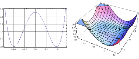
(a) Graph of ${P}(y_{1})$               (b) Graph of ${P}(y_{1},y_{2})$

Figure 1: Graphs of $P(Y)$ for logistic equation $y^{\prime}=ry(1-y)$ with $r=4$, $\delta=0.5$, $y_{0}=1.2$.

The least squares method for solving nonlinear initial value problems was studied by Neuberger and Renka Neuberger and Renka (2005) in 2004. By using a method of steepest descent with a Sobolev gradient, their numerical method for Lorenz equations produces a simple smooth curve that terminates at a stationary point rather than producing the butterfly attractor and they claimed: As far as we know this is the first method that produces a non-chaotic orbit.

Generally speaking, if the nonlinear algebraic equation (2) has $K$ solutions for each $Y_{k}$, the nonconvex target function $P(Y)$ could have about $K^{n}$ minimizers. Conventional optimization methods such as Newton or quasi-Newton type of techniques are local approaches, which can only assure the convergence to one of local solutions. Similar to the Runge-Kutta iterative method, these local solutions depend sensitively on initial data and numerical errors. It was discovered by Gao and Ogden in Gao and Ogden (2008) that if a nonlinear ODE system is subjected to an alternative external force field, both the local and global minimum solutions could be nonsmooth and can’t be captured by Newton-Type direct methods. Due to the lack of global optimality criteria, most nonconvex minimization problems are considered to be NP-hard (Nondeterministic method Polynomial-time Hard). Therefore, from the point view of global optimization and computational complexity theory, we now easily understand that Neuberger and Renka’s smooth curve is only a local stationary solution to the nonconvex minimization problem (3). How to solve a general nonconvex minimization problem has been a fundamentally challenging task not only in global optimization and computer science, but also in multidisciplinary fields of complex systems.

Canonical duality theory is a potentially powerful methodological theory developed from nonconvex analysis/mechanics and global optimization Gao (2000, 2009a). This theory can be used not only to model complex systems within a unified framework, but also for solving a large class of nonconvex/nonsmooth/discrete optimization problems in multidisciplinary fields of computational biology, ecology Ruan and Gao (2014a), engineering sciences Gao (2009a); Wang et al. (2012), and recently in network communications Latorre (2014); Ruan and Gao (2014b), nonconvex constrained optimization Latorre and Gao (2015); Latorre and Sagratella (2014), and radial basis neural networks Latorre and Gao (2014), etc. Comprehensive reviews on the canonical duality theory are given in Gao (2009b); Gao et al. (2014). The main goal of this paper is to apply the canonical duality theory for solving the nonconvex minimization problem (3). The next section provides detailed information on how to reformulate $({\cal P})$ as a concave maximization dual problem and what is the global optimality condition. Numerical method and perturbation technique are discussed in Section 3. Based on the canonical duality theory, a conjecture is proposed which reveals the connection between chaos in nonlinear dynamics and NP-hardness in computer science. Applications are illustrated in Section 4. The methodology and conjecture are tested by three well-known systems. The first one is one-D logistic equation, it has a unique global optimal trajectory. The second one is a two-D forced memristive circuit. This system possesses chaotic behavior by conventional iterative method Itoh and Chua (2011). But by the canonical duality theory, this system has global optimal solutions for different initial data and parameters. The final example is the classical 3-D Lorenz system with the butterfly chaotic attractor. The canonical duality theory shows reason why this well-known chaotic system is NP-hard. Conclusions are presented in the last section.

II Canonical Duality Theory and Global Optimality Condition

The canonical duality theory is composed mainly of (1) a canonical transformation; (2) a complementary-dual principle; (3) a triality theory. To simplify the exposition, we assume that the nonlinear operator $F(t,Y)$ is a vector-valued quadratic function of $Y$:

$$F(t,Y)={Y}^{T}{\bf A}{Y}+{\bf D}{Y}+{\bf g}(t),$$

where ${\bf g}(t)=\{g_{i}(t)\}\in\mathbb{R}^{d}$ is a given vector-valued function, ${\bf A}=\{{\bf A}^{i}_{jl}\}\in\mathbb{R}^{d\times d\times d}$ and ${\bf D}=\{D_{ij}\}\in\mathbb{R}^{d\times d}$ are given generalized matrices, respectively. Thus, the target function ${P}({\bf Y})$ is a fourth-order polynomial of ${\bf Y}\in\mathbb{R}^{d\times n}$:

$${P}({\bf Y})=\frac{1}{2}\sum_{k=1}^{n}\left\|\Lambda({Y}_{k})+{\bf B}({Y}_{k})+{\bf c}_{k}\right\|^{2},$$ (5)

where ${\bf B}({Y}_{k})=\frac{\delta}{2}{\bf D}({Y}_{k}+{Y}_{k-1})-{Y}_{k}+{Y}_{k-1}$, ${\bf c}_{k}=\frac{\delta}{2}({\bf g}_{k}+{\bf g}_{k-1})$, and

$$\Lambda({Y}_{k})=\frac{\delta}{2}({Y}_{k}^{T}{\bf A}{Y}_{k}+{Y}_{k-1}^{T}{\bf A}{Y}_{k-1}).$$ (6)

The key idea of the canonical dual transformation is to choose a certain geometrically admissible non-linear measure such that the high-order nonconvex target function can be written in a canonical function in dual space. By the definition used in the canonical duality theory, a real-valued function $V:{\cal E}_{a}\rightarrow\mathbb{R}$ is said to be a canonical function on its domain ${\cal E}_{a}$ if the canonical dual mapping $\mbox{\boldmath$\sigma$}=\nabla V({\mbox{\boldmath$\xi$}}):{\cal E}_{a}\rightarrow{\cal E}^{*}_{a}$ is one-to-one and onto. For the fourth-order polynomial ${P}({\bf Y})$, such a geometrical operator can be chosen as

$${\bf E}=\{{\mbox{\boldmath$\xi$}}_{k}\}=\{\xi^{i}_{k}\}=\Lambda({\bf Y})=\{\Lambda({Y}_{k})\}:{\cal Y}_{a}\rightarrow{\cal E}_{a}\subseteq\mathbb{R}^{d\times n}.$$ (7)

Thus, a bi-quadratic (canonical) function $\mathbb{R}^{d\times n}\times{\cal E}_{a}\rightarrow\mathbb{R}$ can be defined by

$$\Phi({\bf Y},{\bf E})=\frac{1}{2}\sum_{k=1}^{n}\left\|{\mbox{\boldmath$\xi$}}_{k}+{\bf B}({Y}_{k})+{\bf c}_{k}\right\|^{2}.$$ (8)

In terms of the geometrical operator ${\bf E}=\Lambda({\bf Y})$, the primal problem $({\cal P})$ can be equivalently written in the canonical form

$$({\cal P}):\;\;\;\min\{\Pi({\bf Y})=\Phi({\bf Y},\Lambda({\bf Y}))\;|\;\;\forall{\bf Y}\in{\cal Y}_{a}\}.$$ (9)

By the fact that for any given ${\bf Y}\in{\cal Y}_{a}$, the canonical function $\Phi({\bf Y},{\bf E})$ is convex in ${\bf E}$, the canonical dual variable ${\bf S}\in{\cal E}^{*}_{a}\subset\mathbb{R}^{d\times n}$ can be uniquely defined by

$$\begin{array}[]{rl}{\bf S}&\displaystyle=\{\mbox{\boldmath$\sigma$}_{k}\}=\{\sigma^{i}_{k}\}=\nabla_{{\bf E}}\Phi({\bf Y},{\bf E})\vspace{0.5em}\\ &={\bf E}+{\bf B}({\bf Y})+{\bf C}=\{{\mbox{\boldmath$\xi$}}_{k}+{\bf B}({Y}_{k})+{\bf c}_{k}\},\end{array}$$ (10)

where ${\cal E}^{*}_{a}$ is the range of $\nabla_{{\bf E}}\Phi({\bf Y},{\bf E})$. For a given ${\bf Y}\in{\cal Y}_{a}$, the conjugate function $\Phi^{*}({\bf Y},{\bf S})$ can be defined by the (partial) Legendre transformation

$$\Phi^{*}({\bf Y},{\bf S}) = \{\mbox{tr}({\bf E}^{T}{\bf S})-\Phi({\bf Y},{\bf E})\;|\;\;{\bf S}=\nabla_{{\bf E}}\Phi({\bf Y},{\bf E})\}$$ (11)

$$= \ \sum_{k=1}^{n}\left[\frac{1}{2}\|\mbox{\boldmath$\sigma$}_{k}\|^{2}-\mbox{\boldmath$\sigma$}^{T}_{k}{\bf B}({Y}_{k})-{\bf c}_{k}^{T}\mbox{\boldmath$\sigma$}_{k}\right],$$

where $\mbox{tr}=$trace. Clearly, for any given ${\bf Y}\in{\cal Y}_{a}$, the conjugate $\Phi^{*}({\bf Y},{\bf S})$ is a canonical function of ${\bf S}$ and we have the following canonical duality relations:

$${\bf S}=\nabla_{{\bf E}}\Phi({\bf Y},{\bf E})\;\;\Leftrightarrow\;\;{\bf E}=\nabla_{{\bf S}}\Phi^{*}({\bf Y},{\bf S})\;\;\Leftrightarrow$$

$$\Phi({\bf Y},{\bf E})+\Phi^{*}({\bf Y},{\bf S})=\mbox{tr}({\bf E}^{T}{\bf S})\;\;\forall{\bf Y}\in{\cal Y}_{a}.$$ (12)

The equation (12) is the so-called Fenchel-Young equality, by which, the canonical function $\Phi({\bf Y},\Lambda({\bf Y}))$ can be written in Gao-Strang’s total complementary function:

$$\Xi({\bf Y},{\bf S}) = \mbox{tr}(\Lambda({\bf Y})^{T}{\bf S})-\Phi^{*}({\bf Y},{\bf S})\}$$ (13)

$$= \sum_{k=1}^{n}\Bigg{[}\frac{1}{2}{Y}^{T}_{k}{\bf G}(\mbox{\boldmath$\sigma$}_{k}){Y}_{k}-{Y}^{T}_{k}{\bf t}(\mbox{\boldmath$\sigma$}_{k})$$

$$-\frac{1}{2}\|\mbox{\boldmath$\sigma$}_{k}\|^{2}+{\bf c}^{T}_{k}\mbox{\boldmath$\sigma$}_{k}\Bigg{]}+\psi(\mbox{\boldmath$\sigma$}_{1}),\;\;\;\;\;$$

where ${\bf G}\in\mathbb{R}^{d\times d}$, ${\bf t}\in\mathbb{R}^{d}$, and $\psi(\mbox{\boldmath$\sigma$}_{1})\in\mathbb{R}$ are defined by

$${\bf G}(\mbox{\boldmath$\sigma$}_{k}) = \left\{\sum_{i=1}^{d}{\bf A}^{i}(\sigma^{i}_{k}+\sigma^{i}_{k+1})\right\}$$ (15)

$$\;\;\forall\;\;k=1,\dots,n-1$$

$${\bf G}(\mbox{\boldmath$\sigma$}_{n}) = \left\{\sum_{i=1}^{d}{\bf A}^{i}\sigma^{i}_{n}\right\}$$ (16)

$${\bf t}(\mbox{\boldmath$\sigma$}_{k}) = \left\{\sigma^{i}_{k}-\sigma^{i}_{k+1}-\frac{\delta}{2}\sum_{j=1}^{d}D_{ji}(\sigma^{j}_{k+1}+\sigma^{j}_{k})\right\}$$ (17)

$$\;\;\forall i=1,\dots,d,\;\;\forall k=1,\dots,n-1$$

$${\bf t}(\mbox{\boldmath$\sigma$}_{n}) = \left\{\sigma^{i}_{n}-\frac{\delta}{2}\sum_{j=1}^{d}D_{ji}\sigma^{j}_{n}\right\}\;\;\forall i=1,\dots,d$$ (18)

$$\psi(\mbox{\boldmath$\sigma$}_{1}) = {Y}_{0}^{T}\mbox{\boldmath$\sigma$}_{1}+\frac{\delta}{2}({Y}_{0}^{T}{\bf A}{Y}_{0}+{\bf D}{Y}_{0})\mbox{\boldmath$\sigma$}_{1}.$$ (19)

It is easy to see that $\Xi:{\cal Y}_{a}\times{\cal E}^{*}_{a}\rightarrow\mathbb{R}$ is a bi-quadratic function, by which, the canonical dual function can be obtained by

$$\Pi^{d}({\bf S}) = \left\{\Xi({\bf Y},{\bf S})|\;\;\nabla_{{\bf Y}}\Xi({\bf Y},{\bf S})=0\;\;\forall{\bf S}\in{\cal E}^{*}_{a}\right\}$$ (20)

$$= \sum_{k=1}^{n}\Bigg{[}-\frac{1}{2}{\bf t}(\mbox{\boldmath$\sigma$}_{k})^{T}{\bf G}(\mbox{\boldmath$\sigma$}_{k})^{-1}{\bf t}(\mbox{\boldmath$\sigma$}_{k})$$

$$-\frac{1}{2}\|\mbox{\boldmath$\sigma$}_{k}\|^{2}+{\bf c}^{T}_{k}\mbox{\boldmath$\sigma$}_{k}\Bigg{]}+\psi(\mbox{\boldmath$\sigma$}_{1}).\;\;\;\;\;$$

Let ${\cal S}_{a}=\{{\bf S}\in{\cal E}^{*}_{a}|\;\;\det{\bf G}(\mbox{\boldmath$\sigma$}_{k})\neq 0\;\;\forall k=1,\dots,n\}$ be an admissible dual space, on which, the canonical dual function $\Pi^{d}({\bf S})$ is well-defined.

Theorem 1

$($Complementarity-Dual Principle Gao (2000)$)$ The function $\Pi^{d}({\bf S})$ is canonically dual to $\Pi({\bf Y})$ in the sense that if $\bar{\bf S}$ is a critical point of $\Pi^{d}({\bf S})$ then

$$\bar{{\bf Y}}({\bar{\bf S}})=\{{\bf G}^{-1}(\bar{}\mbox{\boldmath$\sigma$}_{k}){\bf t}(\bar{}\mbox{\boldmath$\sigma$}_{k})\}$$ (21)

is a critical solution to $({\cal P})$ and

$$\Pi(\bar{{\bf Y}})=\Xi(\bar{{\bf Y}},\bar{\bf S})=\Pi^{d}(\bar{\bf S}).$$

Conversely, if $\bar{{\bf Y}}$ is a solution to the nonlinear algebraic system $({\cal P}_{0})$, it must be in the form (21) for certain critical point $\bar{\bf S}$ of $\Pi^{d}({\bf S})$.

This theorem shows that there is no duality gap between the nonconvex target function $\Pi({\bf Y})$ and its canonical dual $\Pi^{d}({\bf S})$, and the local solutions to the nonlinear algebraic system $({\cal P}_{0})$ can be analytically represented in the canonical dual solution. Note that the dual feasible set ${\cal S}_{a}$ is not convex, then in order to find both local and global minimum solutions, we need to introduce the following subsets of ${\cal E}^{*}_{a}$:

$${\cal S}^{+}_{a} = \{{\bf S}=\{\mbox{\boldmath$\sigma$}_{k}\}\in{\cal E}^{*}_{a}|\;{\bf G}(\mbox{\boldmath$\sigma$}_{k})\succeq 0\;\;\forall k=1,\dots,n\},$$

$${\cal S}^{-}_{a} = \{{\bf S}=\{\mbox{\boldmath$\sigma$}_{k}\}\in{\cal E}^{*}_{a}|\;{\bf G}(\mbox{\boldmath$\sigma$}_{k})\prec 0\;\;\forall k=1,\dots,n\}.$$

By the fact that the block matrix ${\bf G}(\mbox{\boldmath$\sigma$}_{k})$ in ${\cal S}^{+}_{a}$ is allowed to be singular ($\det{\bf G}(\mbox{\boldmath$\sigma$}_{k})=0$), the term ${\bf G}(\mbox{\boldmath$\sigma$}_{k})^{-1}$ in $\Pi^{d}({\bf S})$ should be understood as the Moore-Penrose pseudoinverse Gao (2009b).

Theorem 2

$($Triality Theory Gao (2000)$)$ Let $(\bar{{\bf Y}},\bar{\bf S})$ be an isolated critical point of $\Xi({\bf Y},{\bf S})$. The following three extremality conditions hold:

1. Global Optimum: The critical point $\bar{{\bf Y}}$ is a global minimizer of $\Pi({\bf Y})$ if and only if $\bar{\bf S}\in{\cal S}_{a}^{+}$. In this case, we have

   $$\,\,\,\,\,\,\,\,\,\,\,\,\,\,\,\,\min_{{\bf Y}\in{\cal Y}_{a}}\Pi({\bf Y})=\Pi(\bar{{\bf Y}})=\Pi^{d}(\bar{\bf S})=\max_{{\bf S}\in{\cal S}_{a}^{+}}\Pi^{d}({\bf S}).$$ (22)

2. Local Maximum: If $\bar{\bf S}\in{\cal S}_{a}^{-}$, then $\bar{\bf S}$ is a local maximizer of $\Pi^{d}({\bf S})$ on its neighborhood ${\cal S}_{o}\subset{\cal S}_{a}^{-}$ if and only if $\bar{{\bf Y}}$ is a local maximizer of $\Pi({\bf Y})$ on its neighborhood ${{\cal Y}}_{o}\in{\cal Y}_{a}$. In this case, we have

   $$\,\,\,\,\,\,\,\,\,\,\,\,\,\,\,\,\,\max_{{\bf Y}\in{{\cal Y}}_{o}}\Pi({\bf Y})=\Pi(\bar{{\bf Y}})=\Pi^{d}(\bar{\bf S})=\max_{{\bf S}\in{\cal S}_{o}}\Pi^{d}({\bf S}).$$ (23)

3. Local Minimum: If $\bar{\bf S}\in{\cal S}_{a}^{-}$, then $\bar{\bf S}$ is a local minimizer of $\Pi^{d}({\bf S})$ on its neighborhood ${\cal S}_{o}\subset{\cal S}_{a}^{-}$ if and only if $\bar{{\bf Y}}$ is a local minimizer of $\Pi({\bf Y})$ on its neighborhood ${{\cal Y}}_{o}\in{\cal Y}_{a}$. In this case, we have

   $$\,\,\,\,\,\,\,\,\,\,\,\,\,\,\,\,\,\min_{{\bf Y}\in{{\cal Y}}_{o}}\Pi({\bf Y})=\Pi(\bar{{\bf Y}})=\Pi^{d}(\bar{\bf S})=\min_{{\bf S}\in{\cal S}_{o}}\Pi^{d}({\bf S}).$$ (24)

The first statement (22) is called canonical min-max duality. Its was developed from Gao and Strang’s work in 1989 Gao and Strang (1989). This duality can be used to identify global minimizer of the nonconvex problem $({\cal P})$. According this statement, the nonconvex problem $({\cal P})$ is equivalent to the following canonical dual problem, denoted by $({\cal P}^{d})$:

$$({\cal P}^{d}):\;\;\;\max\mbox{sta}\{\Pi^{d}({\bf S})|\;{\bf S}\in{\cal S}_{a}^{+}\},$$ (25)

i.e. to find the global maximizer among all stationary points of $\Pi^{d}({\bf S})$ on ${\cal S}^{+}_{a}$. By the fact that the canonical dual $\Pi^{d}({\bf S})$ is a strictly concave function over a close convex domain ${\cal S}^{+}_{a}$, this canonical dual problem can be solved easily by well-developed convex analysis and optimization techniques if ${\cal S}^{+}_{a}\neq\emptyset$. The solution obtained by this statement provides a global optimal trajectory for the nonlinear system $(IVP)$.

The second statement (23) is the canonical double-max duality and the third one (24) is the canonical double-min duality. These two statements can be used to identify the two special local extremum solutions ${\bf Y}^{\sharp}$ and ${\bf Y}^{\flat}$ such that $\Pi({\bf Y}^{\sharp})\geq\Pi(\bar{\bf Y})$ for all stationary solutions ${\bar{\bf Y}}$ and $\Pi({\bf Y}^{\flat})\geq\Pi({\bar{\bf Y}})$ for all local minimizers ${\bar{\bf Y}}$. By the fact that ${\bf Y}^{\sharp}$ is not a solution to $({\cal P}_{0})$, the local minimum solution ${\bf Y}^{\flat}$ determined by (24) could be useful for understanding the most unstable trajectory in chaos.

III Numerical Methodology and Criteria for Chaos and NP-hardness

This section has two goals: 1) to propose a methodology for solving the canonical dual problem $({\cal P}^{d})$; 2) to find criteria for identify chaos and NP-hard problems.

Theorem 2 shows that there are different approaches for solving the nonconvex primal problem $({\cal P})$. One is to directly solve the dual problem $({\cal P}^{d})$, but this approach has two main disadvantages:

• It is necessary to calculate the inverses of matrices ${\bf G}(\mbox{\boldmath$\sigma$}_{k})$ for $k=1,\dots,n$ every time the target function is evaluated, and such operation could be necessary several times per iteration;

• To compute the inverse matrix can be time expensive or generate errors in the case even one of the ${\bf G}(\mbox{\boldmath$\sigma$}_{k})$ for $k=1,\dots,n$ is either ill-conditioned or not full rank.

For these reasons we propose a canonical primal-dual method for solving the challenging nonlinear system $(IVP)$.

From Theorem 1 it is clear that there is a one to one correspondence among the stationary points of $\Pi({\bf Y})$, $\Pi^{d}({\bf S})$ and $\Xi({\bf Y},{\bf S})$. Therefore it is possible to find a global optimum for Problem (3) by solving the following saddle-point problem ($(SP)$ in short):

$$(SP):\;\;\;\min_{{\bf Y}\in{\cal Y}_{a}}\max_{{\bf S}\in{\cal S}_{a}^{+}}\Xi({\bf Y},{\bf S})=\max_{{\bf S}\in{\cal S}_{a}^{+}}\min_{{\bf Y}\in{\cal Y}_{a}}\Xi({\bf Y},{\bf S}).$$ (26)

Methods for solving saddle point problems have been extensively studied in literature Benzi et al. (2005). One of the most used approaches is to reformulate the (26) as a variational inequality problem on a closed convex set (cone):

$$\Gamma({\bf Y},{\bf S})=\left(\begin{array}[]{c}\nabla_{{\bf Y}}\Xi({\bf Y},{\bf S})\\ -\nabla_{{\bf S}}\Xi({\bf Y},{\bf S})\\ \end{array}\right)=0\;\;\forall\;{\bf S}\in{\cal S}^{+}_{a}.$$ (27)

By the fact that the operator $\Gamma$ is monotone and the feasible set ${\cal S}^{+}_{a}$ is convex, this problem is equivalent to a convex minimization and the solution of (27) can be obtained easily.

In the case that the canonical dual solutions are located on the boundary of ${\cal S}_{a}^{+}$, perturbation methods can be suggested Gao and Ruan (2010); Ruan and Gao (2014c). The simplest perturbation problem is the following:

$$({\cal P}_{\rho}):\;\;\Pi_{\rho}({\bf Y})=\Pi({\bf Y})+\frac{1}{2}\rho\sum_{k=1}^{n}\|{Y}_{k}\|^{2},$$ (28)

where $\rho>0$ is a perturbation parameter. In this problem, the canonical dual feasible set ${\cal S}^{+}_{a}$ should be replaced by

$$\begin{array}[]{rl}{\cal S}^{+}_{\rho}=&\{{\bf S}\in{\cal E}^{*}_{a}|\;\;{\bf G}_{\rho}(\mbox{\boldmath$\sigma$}_{k})=\vspace{0.5em}\\ &{\bf G}(\mbox{\boldmath$\sigma$}_{k})+\rho{\bf I}_{d}\succeq 0\;\;\forall k=1,\dots,n\},\end{array}$$ (29)

where ${\bf I}_{d}$ is an identity matrix in $\mathbb{R}^{d\times d}$. It is easy to see that as the perturbation parameter $\rho$ is getting larger and larger, the matrices $\{{\bf G}_{\rho}(\mbox{\boldmath$\sigma$}_{k})\}$ become more and more diagonally dominated and positive definite and the primal problem $\Pi_{\rho}({\bf Y})$ becomes convex. On the other hand as $\rho$ is approaching to zero, the perturbed problem and its dual are approaching to their original formulations. Such behavior can be exploited in an optimization method to find a good approximation of the original problem $\Pi({\bf Y})$. As a matter of facts it could be possible to start the optimization with a large enough value of $\rho$ and then lower this value during the iterations in order to reach a good enough approximation solution of $\Pi({\bf Y})$.

The triality theory and the associated canonical primal-dual method have been applied successfully for solving many challenging problems in computational sciences (see Ruan and Gao (2014a, c); Zhang et al. (2011)). For the nonlinear dynamical system $(IVP)$, if its discretized nonlinear algebraic problem $({\cal P}_{0})$ has multiple solutions for certain ${Y}_{k}$, then the primal problem $({\cal P})$ could have multiple global minimizers. Conventional iteration methods for solving $({\cal P}_{0})$ could produce chaos since these methods are sensitive to the initial data and numerical error accumulation. However, by the triality theory we know that the nonconvex minimization problem $({\cal P})$ is not NP-hard if its canonical dual problem $({\cal P}^{d})$ is solvable, i.e. it has solutions in ${\cal S}^{+}_{a}$. These solutions are usually located on the boundary of ${\cal S}^{+}_{a}$, which can be obtained deterministically by perturbation method Ruan and Gao (2014c) if $\mbox{int}{\cal S}^{+}_{a}\neq\emptyset$, i.e. ${\cal S}^{+}_{a}$ has interior. Dually, if $\mbox{int}{\cal S}^{+}_{a}=\emptyset$, the canonical dual problem $({\cal P}^{d})$ is not solvable. In this case, the complementary-dual principle (Theorem 1) shows that the primal problem $({\cal P})$ is equivalent to the following minimum stationary problem:

$$({\cal P}^{d}_{s}):\;\;\min\mbox{sta}\{\Pi^{d}({\bf S})|\;\;{\bf S}\in{\cal S}_{a}\},$$ (30)

i.e. to find the global minimizer among all stationary points of $\Pi^{d}({\bf S})$ on ${\cal S}_{a}$. This is a nonconvex minimization problem over a nonconvex feasible space, which could be really NP-hard. Therefore, a conjecture was proposed in Gao (2007).

Conjecture 1 (NP-hard Criterion)

The problem $({\cal P})$ is NP-Hard if its canonical dual $({\cal P}^{d})$ is not solvable.

This conjecture is important for understanding chaos in nonlinear dynamical systems. By looking at the definitions of ${\cal S}_{a}$ and ${\cal S}_{a}^{+}$, we know that if even one of the matrices ${\bf G}(\mbox{\boldmath$\sigma$}_{k})$ for $k=1,\dots,n$ is indefinite for any given ${\bf S}=\{\mbox{\boldmath$\sigma$}_{k}\}\in{\cal E}^{*}_{a}$, then $\mbox{int}{\cal S}^{+}_{a}=\emptyset$. Also, the existence of the canonical dual solution to $({\cal P}^{d})$ depends on the system inputs ${\bf g}(t)$ (see Ruan and Gao (2014c)). Such empirical behaviors for Problem $({\cal P})$ and its dual $({\cal P}^{d})$ give rise to a new conjecture:

Conjecture 2 (Chaos and NP-Hardness)

The nonlinear system $({\cal P}_{0})$ has chaotic solutions if and only if the optimization problem $({\cal P})$ is NP-Hard, i.e. its canonical dual $({\cal P}^{d})$ is not solvable.

This conjecture reveals the connection between chaos in nonlinear dynamics and NP-hardness in computer science. Based on this conjecture, the triality theory can be used to identify chaotic behaviors of a nonlinear dynamical system in the following ways.

1) If $({\cal P}^{d})$ has a unique solution $\bar{\bf S}\in{\cal S}^{+}_{a}$, the nonlinear system $(IVP)$ is stable and the conventional iteration methods for solving $(IVP)$ shouldn’t produce chaos.

2) If $({\cal P}^{d})$ has multiple solutions on the boundary of ${\cal S}^{+}_{a}$ and $\mbox{int}{\cal S}^{+}_{a}\neq\emptyset$, the nonlinear system $(IVP)$ can be considered as deterministically stable since its global optimal trajectories can be obtained deterministically by the canonical duality theory. But, the conventional iteration methods may produce chaotic “solutions”. This type of chaotic behavior can be called pseudo-chaos which is intrinsic to the numerical error-accumulation of these iteration methods.

3) If $({\cal P}^{d})$ is not solvable, the problem $({\cal P})$ is NP-hard and the nonlinear system $(IVP)$ is chaotic.

The methodology, conjecture and results presented in this section can be numerically verified by examples in the next section.

IV Numerical Experience

This section presents applications of the proposed theory and methodology via three examples:

1. One-D Logistic equation with unique solution in ${\cal S}^{+}_{a}$;

2. Two-D forced memristive circuit with $\mbox{int}{\cal S}^{+}_{a}\neq\emptyset$;

3. Three-D Lorenz system with $\mbox{int}{\cal S}^{+}_{a}=\emptyset$.

As a benchmark we use the standard ode45 routine from matlab, which is based on the Runge-Kutta (R-K) method. For every single instance, we first run the test with ode45 and then use the result as starting point of iteration for the Canonical Duality (CD) methodology. The quality of the results is ascertained by plugging back the numerical results obtained by the two methodologies into the primal function (3). The one with the lower value of the target function is considered to be the trajectory closer to the true solution.

IV.1 Logistic Equation

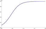
(a) Trajectory by CD methodology.

(b) Trajectory by R-K (ode45).

Figure 2: Comparison of the CD methodology and ode45 for the logistic equation.

For this one-dimensional example, the initial value problem is

$$Y^{\prime}(t)=rY(1-Y),\;\;Y(0)=Y_{0}$$

with the parameter $r=5$ and initial value $Y_{0}=0.1$. As we have already seen in the introduction, such problem is clearly non-convex with more than a local minimum even in its one dimensional version.

It is easy to notice that the matrices ${\bf G}(\sigma_{k})$ for this problem are scalars equal to $(\sigma_{k}+\sigma_{k+1})r$ for $k=1,\dots,n$. The canonical dual variable ${\bf S}=\{\sigma_{k}\}\in\mathbb{R}^{n}$ because of $d=1$. Therefore $\mbox{int}\;{\cal S}_{a}^{+}\neq\emptyset$ as long as $\sigma_{k}+\sigma_{k+1}\geq 0\;\;\forall k=1,\dots,n$ and there exists one $\sigma_{k}>0$. This nonlinear system clearly shows no chaotic behavior and the CD methodology is able to numerically find a global optimal solution in ${\cal S}_{a}^{+}$.

The trajectories by Runge-Kutta (ode45) and the CD methodology are reported in Figures 2(a) and 2(b). The time interval in which the function has been analyzed is $[0,2]$ with step size $\delta=1/500$, i.e. $n=1000$. The target function (3) for the two trajectories takes the following two values:

$$P({Y}_{45})=1.6141e-10,\;\;\quad P({Y}_{CD})=1.1219e-10.$$

From these results it is clear that the two methods are able to give an accurate trajectory of the integral curve $Y(t)$ as the value of the objective function is close to zero. Because of the absence of chaotic behavior, no perturbation has been added to the problem.

IV.2 Forced Memristive Circuit Itoh and Chua (2011)

We now turn our attention on a forced memristive circuit governed by the following nonlinear system Chua and Kang (1976):

$$\begin{array}[]{rl}\displaystyle\frac{dx}{dt}=&\displaystyle a(i^{2}-1),\vspace{0.5em}\\ \displaystyle\frac{di}{dt}=&\displaystyle-(x+\mu)i+\beta\cos(\omega t),\end{array}$$ (31)

where $a,\beta,\mu,\omega$ are given constants. The input term is the applied voltage source $v_{s}(t)=\beta\cos(\omega t)$. Like for the previous example, we analyze the matrices ${\bf G}(\mbox{\boldmath$\sigma$}_{k})$ for $k=1,\dots,n$ that are 2-dimensional matrices:

$$\left(\begin{array}[]{cc}0&-\frac{1}{2}(\sigma^{2}_{k}+\sigma^{2}_{k+1})\\ -\frac{1}{2}(\sigma^{2}_{k}+\sigma^{2}_{k+1})&a(\sigma^{1}_{k}+\sigma^{1}_{k+1})\end{array}\right).$$

The two eigenvalues of this matrix are

$$\begin{array}[]{rl}\lambda_{1,2}^{k}=&\frac{1}{2}a(\sigma^{1}_{k}+\sigma^{1}_{k+1})\vspace{0.5em}\\ &\pm\frac{1}{2}\sqrt{a^{2}(\sigma^{1}_{k}+\sigma^{1}_{k+1})^{2}+(\sigma^{2}_{k}+\sigma^{2}_{k+1})^{2}}.\end{array}$$ (32)

Clearly, the set ${\cal S}^{+}_{a}$ is not empty only if $\sigma^{2}_{k}+\sigma^{2}_{k+1}=0$ for $k=1,\dots,n$. In this case, $\mbox{int}{\cal S}^{+}_{a}\neq\emptyset$ and the problem $({\cal P}^{d})$ could have solutions on the boundary of ${\cal S}^{+}_{a}$. The conventional iterative methods could produce pseudo-chaos, for example, in the case of $x_{0}=0.1,i_{0}=0.1,a=1,\mu=0,\beta=0.7,\omega=1$. But by using the perturbed canonical dual methodology, we are still able to find global optimal trajectory even for this chaotic system. Table 1 shows the global errors $\Pi({\bf Y})$ produced by R-K method (ode45) and perturbed CD method with different step sizes $\delta$, initial values $Y_{0}$, amplitudes $\beta$, and perturbation $\rho$.

n	$Y_{0}$	$\beta$	$\Pi({\bf Y}_{45})$	$\rho_{0}$	$\rho^{*}$	$\Pi({\bf Y}_{CD})$
1000	(0.1,0.1)	0.7	6.4434	1	$1.3841*10^{-2}$	2.8172
10000	(0.1,0.1)	0.7	0.6237	$10^{-2}$	$3.125*10^{-4}$	0.334
100000	(0.1,0.1)	0.7	0.0624	$10^{-3}$	$7.29*10^{-7}$	0.0275
100000	(0.2,0.2)	1	0.0751	$10^{-4}$	$8.1*10^{-7}$	0.0223

Table 1: Global errors $P({\bf Y})$ produced by R-K (ode45) and CD methods for the forced memristive circuit.

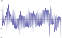
(a) CD solution $x(t)$.

(b) CD solution $i(t)$.

(c) Trajectory by CD methodology.

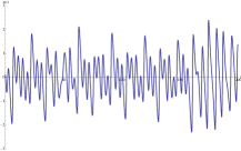
(d) R-K solution $x(t)$ by ode45.

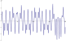
(e) R-K solution $i(t)$ by ode45.

(f) Trajectory by ode45.

Figure 3: Comparisons of the CD methodology and R-K method (ode45) for Eqn (31) with $n=100,000$, $\beta=0.7$, and $Y_{0}=(0.1,0.1)$

Figure 3 shows the chaotic trajectories produced by conventional R-K iteration method with oscillations between $(-3,3)$, see Figure 3 (d). While the global optimal solutions produced by the perturbed canonical dual method are quite more regular and stable with oscillations between $(-0.7,0.7)$, see Figure 3 (c).

The results with changed initial point and amplitude are reported in Figure 4. Compared with Figure 3 we can see that the Runge-Kutta method still produces the pseudo-chaotic “solutions”, while the canonical duality method produces more stable and realistic global optimal solutions.

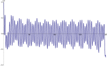
(a) CD solution $x(t)$.

(b) CD solution $i(t)$.

(c) CD trajectory.

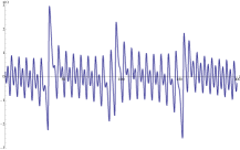
(d) R-K solution $x(t)$ by ode45.

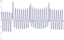
(e) R-K solution of $i(t)$ by ode45.

(f) R-K trajectory by ode45.

Figure 4: Comparisons of the CD methodology and R-K method for Eqn (31) with $n=100,000$, $Y_{0}=(0.2,0.2)$, $\beta=1$

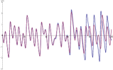
(a) R-K solutions $x(t)$ by ode45 (blue) and ode23 (red).

(b) R-K solutions $i(t)$ by ode45 (blue) and ode23 (red).

Figure 5: Comparisons of R-K solutions for Eqn (31) produced by ode45 and ode23 with $n=100000$ for the memristive circuit. It is possible to see that the two trajectories are diverging with the increasing number of iterations

To further understand the pseudo-chaos due to error-accumulations produced by the conventional iteration methods, we present the chaotic numerical results to the Eqn (31) produced by an another routine ode23 in Matlab, with is also based on Runge-Kutta method. The total error of this solution is $\Pi({\bf Y}_{23})=0.0622$. From Figure 5 we can see that the two trajectories coincide for the first iterations and then, as the numerical error accumulates, they diverge. This fact shows that the conventional iterative methods can’t produce reliable numerical solutions for deterministically stable nonlinear systems due to the intrinsic numerical error accumulations.

IV.3 Lorenz Equations

The Lorenz system has been studied extensively in literature and is well known for its highly chaotic behavior with butterfly attractor Sparrow (2012). This section presents a canonical dual approach to show the reason for chaos and to verify Conjecture 2.

The initial value problem for Lorenz system with standard parameters is

$$\begin{array}[]{rl}\displaystyle\frac{dx}{dt}&\displaystyle=10(y-x),\;\;x(0)=10,\vspace{0.5em}\\ \displaystyle\frac{dy}{dt}&\displaystyle=-xz+28x-y,\;\;y(0)=12,\vspace{0.5em}\\ \displaystyle\frac{dz}{dt}&=\displaystyle xy-\frac{8}{3}z,\;\;z(0)=14.\end{array}$$

In order to understand how ${\cal S}_{a}^{+}$ is characterized, we start the analysis by looking at the matrices ${\bf G}(\mbox{\boldmath$\sigma$}_{k})$ for $k=1,\dots,n$:

$$\left(\begin{array}[]{ccc}0&\frac{1}{2}(\sigma^{3}_{k}+\sigma^{3}_{k+1})&-\frac{1}{2}(\sigma^{2}_{k}+\sigma^{2}_{k+1})\\ \frac{1}{2}(\sigma^{3}_{k}+\sigma^{3}_{k+1})&0&0\\ -\frac{1}{2}(\sigma^{2}_{k}+\sigma^{2}_{k+1})&0&0\end{array}\right).$$

The three eigenvalues can be easily calculated as:

$$\begin{array}[]{rl}\displaystyle\lambda_{1}^{k}&\displaystyle=0\vspace{0.5em},\\ \displaystyle\lambda_{2}^{k}&\displaystyle=\frac{1}{2}\sqrt{(\sigma^{2}_{k}+\sigma^{2}_{k+1})^{2}+(\sigma^{2}_{k}+\sigma^{2}_{k+1})^{2}}\vspace{0.5em},\\ \displaystyle\lambda_{3}^{k}&\displaystyle=-\frac{1}{2}\sqrt{(\sigma^{2}_{k}+\sigma^{2}_{k+1})^{2}+(\sigma^{2}_{k}+\sigma^{2}_{k+1})^{2}}.\\ \end{array}$$ (33)

Equations (33) show that for any ${\bf S}=\{\mbox{\boldmath$\sigma$}_{k}\}\in{\cal E}^{*}_{a}$, the global matrix $\{{\bf G}(\mbox{\boldmath$\sigma$}_{k})\}$ has total $n$ zero eigenvalues, $n$ positive eigenvalues and $n$ negative eigenvalues. Therefore ${\bf G}(\mbox{\boldmath$\sigma$}_{k})$ is indefinite for any dual variable ${\bf S}=\{\mbox{\boldmath$\sigma$}_{k}\}\in{\cal E}^{*}_{a}$, thus both $\mbox{int}\;{\cal S}_{a}^{+}$ and ${\cal S}^{-}_{a}$ are empty for the Lorenz system. By Conjecture 1 we know that the problem $({\cal P})$ is NP-hard. This explains the highly chaotic behavior of the Lorenz system and verifies Conjecture 2.

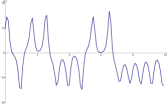
(a) CD solution $x(t)$ using initial iteration produced by ode45.

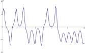
(b) R-K solution $x(t)$ by ode45.

Figure 6: Comparison between the CD methodology and ode45 for the Lorenz system

By the fact that $\mbox{int}\;{\cal S}^{+}_{a}=\emptyset$ for the Lorenz system, we have to solve the nonconvex canonical dual problem $({\cal P}^{d}_{s})$ defined by (30), which is NP-hard and numerical solutions depend sensitively on the initial iteration. We have performed the test for time interval $[0,10]$ with step size $\delta=1/1000$, i.e. $n=10,000$. First we run ode45 and then use the numerical result by Runge-Kutta (R-K solution) as a starting point for the canonical dual iteration. The numerical solutions for $x(t)$ are reported in Figures 6(a) and 6(b). It is possible to see that the two trajectories are quite similar, but the main difference is the total errors:

$$\Pi({\bf Y}_{45})=10^{-3},\;\;\;\quad\Pi({\bf Y}_{CD})=3.326*10^{-07},$$

i.e., the total error produced by CD method is much smaller than the one produced by R-K method. By the fact that ${\cal S}_{a}^{+}$ has no-interior, we can’t theoretically claim that ${\bf Y}_{CD}$ is a global minimum solution to Problem (3) for the Lorenz equations, however, the fact that $\Pi({\bf Y}_{CD})\simeq 0$ indicates that the canonical dual solution ${\bf Y}_{CD}$ is indeed one of global optimal solutions to the nonlinear system $({\cal P}_{0})$. By Conjecture 2 we can say that the Lorenz system is chaotic and the CD method produces the well-known butterfly trajectories as shown in Figure 7.

(a) Trajectory produced by ode45.

(b) Trajectory produced by CD method.

Figure 7: Lorenz attractors produced by ode45 (left) and the CD methodology (right)

.

Finally in Figure 8 we report the trajectories produced by the perturbed CD methodology starting from the origin for the values of the primal variables. In detail:

• the Yellow curve represents the solutions for $x(t)$ with $\rho=10^{-3}$ and $\Pi_{\rho}({\bf Y}^{*})=4.9$;

• The red curve represents the solutions for $x(t)$ with $\rho=10^{-5}$ and $\Pi_{\rho}({\bf Y}^{*})=2.5$;

• The blue curve represents the solutions for $x(t)$ with $\rho=10^{-6}$ and $\Pi_{\rho}({\bf Y}^{*})=1.6$;

We can see that all of these trajectories are stable even after changing the value of $\rho$. Therefore we can state that if the algorithm by the CD methodology starts from a generic point in ${\cal S}_{\rho}^{+}$ with an high enough value of $\rho$ it reaches a stable trajectory. On the other side, because of the characterization of the original ${\cal S}_{a}^{+}$, the error is quite high, far from the theoretical optimal value that is zero. Nevertheless such trajectories correspond to local solutions of Problem (3).

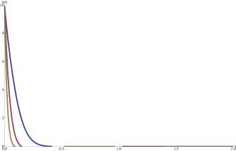
Figure 8: Perturbed CD solutions $x(t)$ starting from the origin with $\rho=10^{-6}$ (blue), $\rho=10^{-5}$ (red), and $\rho=10^{-3}$ (yellow).

V Conclusions

We have presented a nonconventional method for solving nonlinear dynamical systems. Based on the methods of finite differences and least squares, the nonlinear initial value problem is first reformulated as a global minimization problem. By using the canonical duality theory, the nonconvex minimization problem is able to converted to a concave maximization dual problem over a convex cone ${\cal S}^{+}_{a}$. The triality theory shows that if $\mbox{int}\;{\cal S}^{+}_{a}\neq\emptyset$, the global optimal solution can be obtained deterministically in polynomial time. Otherwise, the primal problem could be NP-hard and the nonlinear system could have chaotic behavior. A conjecture is proposed, which reveals the connection between chaos in nonlinear dynamics and NP-hardness in computer science. The method and the conjecture are verified by three examples. Computational results show that the conventional linear iteration methods can’t produce reliable solutions due to the intrinsic numerical error accumulations; while the canonical duality theory can be used not only to identify chaotic systems, but also for obtaining global optimal solutions to general nonlinear dynamic systems.

References

- Ruan et al. (2010) N. Ruan, D. Y. Gao, and Y. Jiao, Computational Optimization and Applications 47, 335 (2010).
- Neuberger and Renka (2005) J. Neuberger and R. Renka, Nonlinear Anal. Convexity 6, 65 (2005).
- Gao and Ogden (2008) D. Gao and R. Ogden, QJ Mech. Appl. Math 61, 497 (2008).
- Gao (2000) D. Y. Gao, Duality principles in nonconvex systems: theory, methods and applications, vol. 39 (Springer Science & Business Media, 2000).
- Gao (2009a) D. Gao, Comput. Chem 33, 1964 (2009a).
- Ruan and Gao (2014a) N. Ruan and D. Y. Gao, IMA Journal of Applied Mathematics 79, 313 (2014a).
- Wang et al. (2012) Z. Wang, S.-C. Fang, D. Y. Gao, and W. Xing, Journal of Global Optimization 54, 341 (2012).
- Latorre (2014) V. Latorre, arXiv preprint arXiv:1403.5991 (2014).
- Ruan and Gao (2014b) N. Ruan and D. Y. Gao, Performance Evaluation 75, 1 (2014b).
- Latorre and Gao (2015) V. Latorre and D. Gao, Optimization Letters pp. 1–17 (2015), ISSN 1862-4472, URL http://dx.doi.org/10.1007/s11590-015-0860-0.
- Latorre and Sagratella (2014) V. Latorre and S. Sagratella, Journal of Global Optimization pp. 1–17 (2014), ISSN 0925-5001, URL http://dx.doi.org/10.1007/s10898-014-0236-5.
- Latorre and Gao (2014) V. Latorre and D. Y. Gao, Neurocomputing 134, 189 (2014).
- Gao (2009b) D. Y. Gao, Computers & Chemical Engineering 33, 1964 (2009b).
- Gao et al. (2014) D. Y. Gao, N. Ruan, and V. Latorre, http://arxiv.org/abs/1410.2665 p. 1081286514566533 (2014).
- Itoh and Chua (2011) M. Itoh and L. O. Chua, International Journal of Bifurcation and Chaos 21, 2395 (2011).
- Gao and Strang (1989) Y. Gao and G. Strang (Brown University, 1989), vol. 47, pp. 487–504.
- Benzi et al. (2005) M. Benzi, G. H. Golub, and J. Liesen, Acta numerica 14, 1 (2005).
- Gao and Ruan (2010) D. Y. Gao and N. Ruan, Journal of Global Optimization 47, 463 (2010).
- Ruan and Gao (2014c) N. Ruan and D. Y. Gao, Performance Evaluation 75, 1 (2014c).
- Zhang et al. (2011) J. Zhang, D. Y. Gao, and J. Yearwood, Journal of theoretical biology 284, 149 (2011).
- Gao (2007) D. Y. Gao (2007).
- Chua and Kang (1976) L. O. Chua and S. M. Kang, Proceedings of the IEEE 64, 209 (1976).
- Sparrow (2012) C. Sparrow, The Lorenz equations: bifurcations, chaos, and strange attractors, vol. 41 (Springer Science & Business Media, 2012).