Exponential system-size dependence of the lifetime of transient spiral chaos
in excitable and oscillatory media

Abstract

Excitable media can develop spiral chaos, in which the number of spirals changes chaotically with time. Depending on parameter values in dynamical equations, spiral chaos may permanently persist or spontaneously arrive at a steady state after a transient time, referred to as the lifetime. Previous numerical studies have demonstrated that the lifetime of transient spiral chaos increases exponentially with system size to a good approximation. In this study, using the fact that the number of spirals obeys a Gaussian distribution, we provide a general expression for the system size dependence of the lifetime for large system sizes, which is indeed exponential. We confirm that the expression is in good agreement with numerically obtained lifetimes for both excitable and oscillatory media with parameter sets near the onset of transient chaos. The expression we develop for the lifetime is expected to be useful for predicting lifetimes in large systems.

I INTRODUCTION

Excitable media play vital roles in various systems Winfree (1980); Keener and Sneyd (2009); Cross and Hohenberg (1993). Excitable media in biological tissues support the propagation of signals, such as concentration waves in the heart and electrical impulses in nerve axons. Such waves are also used for communication between certain microorganisms (Dictyostelium discoideum).

Moreover, excitable media exhibit a particular type of spatiotemporal chaotic dynamics, in which spiral waves spontaneously generate or annihilate (spiral chaos) Winfree (1980); Kuramoto (1984). Spiral chaos is commonly observed in surface reaction systems Beta et al. (2006); Bär and Eiswirth (1993). Similar chaotic dynamics are also observed in the heart, causing fibrillation Qu (2006). So far, several mathematical models for excitable media that exhibit spiral chaos have been proposed Bär and Eiswirth (1993); Qu (2006); Krefting and Beta (2010).

It is also known that spiral chaos may develop in oscillatory media, e.g., those obeying the complex Ginzburg-Landau equation (CGLE) Kuramoto (1984); Chaté and Manneville (1996); Krefting and Beta (2010); Berenstein and Beta (2011). In such mathematical models, depending on the parameter values, spiral chaos permanently persists or spontaneously terminates (Fig. 1). In the latter case, the system eventually arrives at a steady state after a transient time, which we refer to as a lifetime. The dependence of the lifetime of spiral chaos on the system size has received much attention in the context of the clinical treatment of cardiac fibrillation (Qu (2006) and the references therein). In Qu (2006), it is numerically demonstrated using both a variant of FitzHugh–Nagumo model (referred to as the Bär model Bär and Eiswirth (1993)) and a more realistic model for cardiac electrical dynamics that the lifetime increases exponentially with the system size. Such an exponential dependence, as well as hyperexponential dependences, had already been reported in other types of transient chaos Wackerbauer and Showalter (2003); Tél et al. (2008); Wacker et al. (1995); Crutchfield and Kaneko (1988).

The main focus of the present study is an expression for the dependence of the lifetime of spiral chaos in excitable media on the system size. For this goal, we first investigate statistical properties regarding the number of spiral cores (namely, defects). There is a large body of studies on such statistical properties Gil et al. (1990); Ebata and Sano (2011); Qiao et al. (2009); Davidsen and Kapral (2003); Falcke et al. (1999). In particular, it is known that as system size increases, the probability distribution of the number of defects during transient spiral chaos approaches a Gaussian distribution Davidsen et al. (2005), as is naturally expected from the central limit theorem. Using this fact, we derive an expression for the system size dependence of the lifetime, which is indeed exponential.

We extensively investigate the system size dependence of the lifetime using two different models, the Bär model and the CGLE, with several parameter sets and different boundary conditions. We find that while the lifetime increases exponentially with system size in all cases, our expression fits well for parameter sets near the onset of transient chaos, suggesting that some assumptions may be violated depending on parameter values.

The present paper is organized as follows. In Sec. II, we describe the model and the numerical settings. In Sec. III, we show that the probability distribution of the number of defects approaches a Gaussian distribution as the system size increases. In Sec. IV, we first numerically show that the lifetime of transient spiral chaos increases exponentially with system size; then, we derive the expression for the system size dependence of the lifetime, which fits well to numerical data for some parameter sets. A summary and discussion are provided in Sec. V.

II model and numerical settings

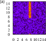
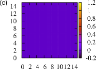
Figure 1: Snapshots of $u(x,y,t)$ in the Bär model. (a) Initial condition ($t=0$) is constructed as follows. First, we create a flat excitation wave, run a simulation for a while, and cut the wave into half. We then add random noise with a uniform probability distribution over $[-0.25,0.25]$. (b) Transient spiral chaos ($t=136$). (c) Uniform steady state ($t=160$). The parameter values are $a=0.84,~{}b=0.07,~{}\epsilon=0.08$, and $N=15^{2}$.

For most of our numerical investigation, we employ the Bär model Bär and Eiswirth (1993), which is a modified FitzHugh–Nagumo model representing an excitable medium. This model has also been employed in Qu (2006). The model gives

$$\frac{\partial{u}}{\partial{t}} = -\frac{1}{\epsilon}u(u-1)\left(u-\frac{v+b}{a}\right)+D\nabla^{2}u,$$ (1a)

$$\frac{\partial{v}}{\partial{t}} = f(u)-v,$$ (1b)

$$f(u) = \begin{cases}0\ ,\ u<\frac{1}{3},\\ 1-6.75u(u-1)^{2}\ ,\ \frac{1}{3}\leq u\leq 1,\\ 1\ ,\ u>1,\end{cases}$$ (1c)

where the parameters $\epsilon,a,b$ and the diffusion coefficient $D$ are positive. The system is two dimensional with an area $L\times L\equiv N$. The variables $u(x,y,t)$ and $v(x,y,t)$ are interpreted in the context of cell physiology as the membrane potential and the recovery variable, respectively Keener and Sneyd (2009). Numerical simulations are performed using the fourth-order Runge–Kutta method with space step $h=0.3$ and time step $s=0.01$.

We first note that in Eq. (1), the uniform steady state $u(x,y)=v(x,y)=0$ is linearly stable for any set of parameter values. By inserting the ansatz $u,v\sim e^{\lambda t-{\rm i}\bm{q}\cdot\bm{r}}$ with $\bm{r}=(x,y)$ and a wave vector $\bm{q}$ of perturbation, we obtain $\lambda=-1,-\frac{b}{a\epsilon}-D|\bm{q}|^{2}$, which is always negative. Hence, the system should smoothly arrive at the uniform steady state if the initial state is close to it.

However, for appropriate parameter values and initial conditions, spatiotemporal chaotic dynamics arise (referred to as spiral chaos) (Fig. 1). As reported in Bär and Eiswirth (1993), for a broad range of $b$ ($b<0.18,a=0.84$), the following behavior arises. For small $\epsilon$ values ($0.01<\epsilon<0.06$), spiral waves rigidly rotate. For $\epsilon>0.06$, spiral waves begin to meander. For $\epsilon>0.07$, spiral chaos arises. In this region, spirals begin to break up after some transient rotations, resulting in the formation of two free ends of a wave. From these free ends, a new pair of counter-rotating spirals arise. There is also a pair-annihilation process, in which the cores of a pair of counter-rotating spirals collide and annihilate. Moreover, in the Neumann boundary condition, there is an additional case in which a defect is absorbed by the boundary. These processes are repeated chaotically.

As a convenient initial condition for realizing this chaotic state, we employ a flat broken wave (Fig. 1), in which there initially exists a defect for the Neumann boundary condition or a pair of defects for the periodic boundary condition. To obtain statistically independent results for each run of the simulations, we add independent random noise obeying a uniform probability distribution over $[-\eta,\eta]$ with $\eta=0.25$ to $u$ and $v$ at all discretized points at $t=0$. Note that the evolution is noise free for $t>0$. In our preliminary numerical simulations, we have checked that our statistical results do no change quantitatively for $\eta=0.1$ (results not shown). The results presented assume the periodic boundary condition and $a=0.84,b=0.07,\epsilon=0.08,D=1$ unless otherwise noted. Some results are obtained with the Neumann boundary condition and/or other sets of $b$ and $\epsilon$ values.

To check the generality of our argument, we also numerically investigate the oscillatory media described by the complex Ginzburg–Landau equation (CGLE), given by

$$\frac{\partial W}{\partial t}=W+(1+{\rm i}c_{1})\nabla^{2}W-(1+{\rm i}c_{2})|W|^{2}W,$$ (2)

where $W(x,y,t)\in\mathbb{C}$ is the state variable and $c_{1},c_{2}\in\mathbb{R}$ are the parameters of this system Kuramoto (1984).

III Time evolution and probability distribution of the number of defects

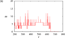
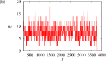
Figure 2: Time series of the number $m(t)$ of defects with system size (a) $N=24^{2}$ and (b) $N=30^{2}$.

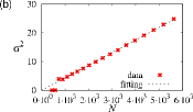
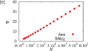
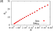
Figure 3: Mean $\mu$ and variance $\sigma^{2}$ of the number of defects. (a, b) Results for the periodic boundary condition. The fitting lines are $\mu=0.00709N$ and $\sigma^{2}=0.00437N$. (c, d) Results for the Neumann boundary condition. The fitting lines are $\mu=0.00660N-1.3996$ and $\sigma^{2}=0.00452N$. Fitting is performed for data with $N>2000$.

We first investigate the time evolution and probability distribution of the number of defects. All the results in this section are for periodic boundary condition. We confirmed that qualitatively the same results were obtained with the Neumann boundary condition.

The number $m(t)$ of defects at time $t$ in the system was counted as follows. The phase $\phi(x,y)$ of the state is defined by $\arg[(u(x,y)-u_{0})+{\rm i}(v(x,y)-v_{0})]$ with $(u_{0},v_{0})=(0.5,0.3)$ and $\arg W$ for the Bär model and the CGLE, respectively. The topological charge $C(x,y,t)$ is defined by $\frac{1}{2\pi}\oint\nabla\phi(\bm{r},t)\cdot d\bm{l}$. The defects with $C=1$ and $-1$ are the cores of counterclockwise and clockwise spirals, respectively. The topological charge is numerically obtained by calculating $C(x,y)=(\phi_{1,2}+\phi_{2,3}+\phi_{3,4}+\phi_{4,1})/2\pi$, where $\phi_{i,j}=\phi_{i}-\phi_{j}$ ($-\pi\leq\phi_{i,j}<\pi$), $\phi_{1}=\phi(x,~{}y)$, $\phi_{2}=\phi(x+h,~{}y)$, $\phi_{3}=\phi(x+h,~{}y+h)$, $\phi_{4}=\phi(x,~{}y+h)$, and $h$ is the space step employed in our numerical simulations. We then reset $C=\pm 1$ when a numerically obtained $C$ value is in $[(\pm 2\pi-0.1)/2\pi,~{}(\pm 2\pi+0.1)/2\pi]$ and $C=0$ otherwise. The number $m(t)$ of defects is the sum of $|C|$ over the entire system.

As seen in Fig. 2, $m(t)$ fluctuates strongly with time, and this chaotic process appears to be stationary. However, defects completely vanish at a certain time without any clear presage, and the system falls into the uniform steady state. As is the case in Figs. 2 (a) and (b), a larger system typically has a larger number of defects and a longer transient time.

Statistical properties are investigated with the time series of $m(t)$ during transient chaos after the initial transient process ($t>100$) (Figs. 3 and 4). Here for each system size, we employ many different initial conditions and the number of defects is counted at each time step until the system arrives at the steady state. We find that both the mean $\mu$ and variance $\sigma^{2}$ of $m(t)$ are approximately proportional to the system size $N$ (Fig. 3):

$$\mu =\alpha N,$$ (3)

$$\sigma^{2} =\beta N.$$ (4)

The linear growth of $\mu$ has also been found in Strain and Greenside (1998). Next, we measure the probability distribution of the number of defects, which is the probability that there are $m$ defects at each time in the system during transient chaos. As is found in Beta et al. (2006), we confirm that the probability distribution approaches the following Gaussian distribution as the system size increases (Fig. 4):

$$p(m) =\frac{\delta}{\sqrt{2\pi{\sigma}^{2}}}\exp\left[-\frac{(m-\mu)^{2}}{2{\sigma}^{2}}\right]$$ (5)

$$=\frac{\delta}{\sqrt{2\pi{\beta}N}}\exp\left[-\frac{(m-\alpha N)^{2}}{2{\beta}N}\right],$$ (6)

where $\delta=1$ for the Neumann boundary condition and $\delta=2$ for the periodic boundary condition because $m$ takes only even number values in the latter case.

These results can be rationalized by the following argument. Suppose that the system is virtually divided into $n$ subsystems of size $\tilde{L}\times\tilde{L}=\tilde{N}$. For the periodic boundary condition, all the subsystems should share a certain probability distribution of the number of defects with mean $\tilde{\mu}$ and variance ${\tilde{\sigma}}^{2}$. If the linear length $\tilde{L}$ of each subsystem is sufficiently larger than the correlation length of the system, these subsystems are approximately independent. In our case, the correlation length is roughly $10$ or smaller (Fig. 5). The number of defects $m$ in the entire system is the sum of defects of independent subsystems. The mean and variance of $m$ are then proportional to the system size. Moreover, as stated by the central limit theorem, $m$ will obey the Gaussian distribution with mean $\mu=n\tilde{\mu}$ and variance $\sigma^{2}=n{\tilde{\sigma}}^{2}$ where $n\equiv\frac{N}{\tilde{N}}$ when $n$ is sufficiently large. This is also approximately the case for the Neumann boundary condition when $L$ is sufficiently larger than the correlation length.

Because this argument is very general, the Gaussian distribution should be obtained for both the periodic and Neumann boundary conditions and other models exhibiting spiral chaos when $N$ is sufficiently large. In fact, we confirmed it for the Bär model and the CGLE with all the parameter sets we chose and both boundary conditions (results not shown).

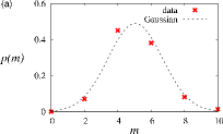
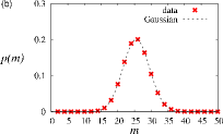
Figure 4: Distribution of the number of defects. (a) System size $N=27^{2}$. (b) $N=60^{2}$. The dashed lines are the Gaussian distributions with average $\mu=\alpha N$ and variance $\sigma^{2}=\beta N$ with $\alpha=0.00709$ and $\beta=0.00437$.

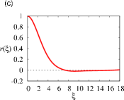
Figure 5: Numerical measurement of correlation length. We estimate the correlation length using two methods. (a, b) The density of defects with (a) $C=-1$ and (b) $C=1$ at $(x,y)$ as a function of the distance $\xi=\sqrt{(x-x_{0})^{2}+(y-y_{0})^{2}}$ from a certain defect with $C=1$ at $(x_{0},y_{0})$ (c) The Pearson product-moment correlation coefficient for the variable $u$, defined as $r(\xi)=\frac{\int_{0}^{T}(u^{*}-\overline{u})(u-\overline{u})dt}{\sqrt{\int_{0}^{T}(u^{*}-\overline{u})^{2}dt}\sqrt{\int_{0}^{T}(u-\overline{u})^{2}dt}},$ where $u^{*}=u(\frac{L}{2},~{}\frac{L}{2},~{}t)$, $u=u(\frac{L}{2}-\xi,~{}\frac{L}{2},~{}t)$ and $\overline{u}$ is the average of $u$ over the entire system. These results indicate that the correlation length is roughly $10$ or less.

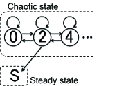
Figure 6: Defect generation-annihilation process for periodic boundary condition. The circle with the number $m$ denotes the state with $m$ defects. The symbol S denotes the uniform steady state.

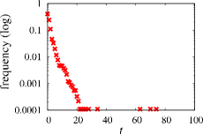
Figure 7: Normalized histogram of the duration in which the number $m$ of defects continues to be zero until $m$ becomes two. Here, the value at $t=k\in\mathbb{N}$ denotes the frequency of the duration $k-1<t\leq k$. The Bär model with $b=0.07,\epsilon=0.09$. Defects seldom reemerge for $t>20$.

IV system size dependence of lifetime

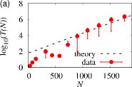
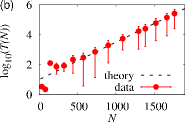
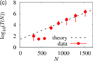
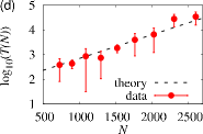
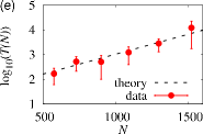
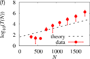
Figure 8: Lifetime $T(N)$ (log scale) vs $N$. The symbol and the error bar correspond to the average and the standard deviation of $T(N)$ for each system size, respectively. (a) Bär model with periodic boundary condition, $b=0.070,~{}\epsilon=0.080$. (b) Bär model with Neumann boundary condition, $b=0.070,~{}\epsilon=0.080$. (c) Bär model with periodic boundary condition, $b=0.030,~{}\epsilon=0.075$. (d) CGLE with periodic boundary condition, $c_{1}=0.80,~{}c_{2}=-1.00$. (e) CGLE with periodic boundary condition, $c_{1}=0.50,~{}c_{2}=-1.11$. (f) Bär model with periodic boundary condition, $b=0.070,~{}\epsilon=0.090$. Note that in the Bär model with the periodic boundary condition (a,c,f), the system size dependence of lifetime is obviously not exponential for small system sizes ($N\leq 24^{2}$). For such small systems, we find that transient chaotic states occasionally end up with various complex patterns including temporally periodic states with $m\neq 0$.

As already mentioned, a previous numerical study reported that the lifetime of transient spiral chaos increases exponentially with the system size. We also numerically confirm it in the following manner.

In any boundary conditions, all the defects must completely vanish before the system settles down to the steady state. Here, it should be noted that there is still a chance that a pair of defects is generated even from the state with $m=0$ because of some remaining complex pattern .

Therefore, the transition between the states with different numbers of defects $m$ can be illustrated as in Fig. 6, where the periodic boundary condition is assumed for simplicity so that $m$ takes only even numbers, and the symbol S denotes the uniform steady state.

To define the lifetime, we regard the system state as the steady state when the duration of the state with $m=0$ continues for 100 simulation time, as defects hardly reemerge if the state with $m=0$ continues for 20 simulation times (Fig. 7). Under such a numerical setup, we investigate the dependence of the lifetime on the system size $N$ (Fig. 8), which is indeed exponential.

The expression for the system size dependence of lifetime $T(N)$ can be obtained as follows. We assume that the process illustrated in Fig. 6 is Markovian. Starting from some initial number $m^{*}$ of defects, we have a series of defect number at each time; e.g., $\{m^{*},m^{*}+2,\cdots,4,4,4,6,6,4,2,2,0,0,2,2,2,{\rm S}\}$, where the symbol “S” denotes the event at which $0$ continues for 100 unit time (which we regard as the steady state). The lifetime at each trial is the length of this series. The expected value of lifetime $T$ is the inverse of the probability $\lambda$ to obtain S. Because S is obtained only when the previous number is $2$, $\lambda=Zp(2)$ where $p(2)$ is the probability to obtain $2$ and $Z$ is the transition rate from the state with $m=2$ to the steady state. Therefore, the expected lifetime for a given system size $N$ is

$$T(N)=\frac{1}{Zp(2)}.$$ (7)

For large $N$, the probability distribution of the number of defects is well approximated by Eq. (6) and the mean number $\mu(=\alpha N)$ of defects is large. For $m\ll\mu$, we approximately have

$$p(m)\sim\exp\left(-\frac{\alpha^{2}}{2\beta}N\right)$$ (8)

Plugging this into $p(2)$ in Eq. (7) and further assuming that $Z$ is independent of $N$, we finally obtain

$$T(N)\sim\exp\left(\frac{\alpha^{2}}{2\beta}N\right).$$ (9)

This expression indicates that the lifetime depends exponentially on the system size $N$ and its exponent is associated with the density $\alpha$ and the magnitude $\beta$ of the fluctuation of the number of defects. For the Neumann boundary condition, the steady state can be reached not only from the states with $m=2$ by annihilation but also from the states with $m=1$ through the absorption of a defect by the boundary. Therefore, the probability $\lambda$ to obtain S is $\lambda=Z_{1}p(1)+Z_{2}p(2)$ with transition rates $Z_{1}$ and $Z_{2}$. In this case as well, we obtain Eq. (9) because both $p(1)$ and $p(2)$ can be well approximated by Eq. (8) for large $N$.

Our expression (9) is numerically verified (Fig. 8). The slope given by Eq. (9) (the dashed lines) is in good agreement with that obtained numerically in both the Bär model (Fig. 8 (a–c)) and the CGLE (Fig. 8(d,e)) for large system sizes.

However, we find discrepancy for some parameter sets. In the Bär model, there are considerable deviations for large $\epsilon$ values (e.g., Fig. 8(f)). In the CGLE, we also find such cases for some parameter sets, e.g., $c_{1}=0.50$, $c_{2}=-1.50$ with the periodic boundary condition (result not shown). All together, we find that the parameter sets for which our theory is valid are typically in the region near the onset of transient chaos Bär and Eiswirth (1993); Chaté and Manneville (1996). A possible reason why our theory fails when the system is far from the onset of spiral chaos will be discussed in Sec. V.

V conclusions and discussion

In the present paper, we have investigated the system size dependence of the lifetime of spiral chaos. We derived an expression for the lifetime, given as Eq. (9), utilizing the fact that the probability distribution of the number of defects is Gaussian for large system sizes. We confirmed that Eq. (9) well fits numerically obtained $T(N)$ for two different models, the Bär model and the CGLE, with several parameter sets and different boundary conditions.

We emphasize that Eq. (9) is useful for the prediction of the lifetime of large systems. We can precisely estimate $\alpha$ and $\beta$ values from observations of the number of defects in a large system. The observation of a relatively small system for different initial conditions enables us to find the average lifetime $T(N)$. Then, using $T(N)\sim\exp\left(\frac{\alpha^{2}}{2{\beta}}N\right)$, we can estimate the average lifetime for large system sizes.

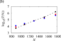
Figure 9: System size dependence of numerically obtained $T$ (symbol $\bullet$ with dashed line), $C_{1}/p(2)$ with numerically obtained $p(2)$ (symbol $\times$) and $C_{2}/p(2)$ with $p(2)$ given by Eq. (8) (symbol $\Box$), where $C_{1}$ and $C_{2}$ are fitting parameters. Parameter values for (a) and (b) are the same as those for Fig. 8(c) and Fig. 8(f), respectively.

We have also found that Eq. (9) fails to predict the system size dependence for the parameter sets far from the onset of chaos. Our theory is based on Eqs. (7) and (8). We can verify these equations by comparing the system size dependences of $T$ and $1/p(2)$ obtained numerically and those predicted by Eqs. (7) and (8). As shown in Fig. 9, whereas both Eqs. (7) and (8) are valid near the onset, discrepancy between numerically obtained $T$ and $1/p(2)$ is particularly large far from the onset. Thus, the assumption in Eq. (7) seems to be violated. Namely, the transition rate $Z$ from the state with $m=2$ to the steady state seems to depend strongly on the system size in such a parameter region.

The following observation may provide reasoning for it. Even when defects completely vanish, some wave pattern may persist for a while. Defect reemergence is attributed to such a remaining pattern Note (1). The complexity of wave patterns in the absence of defects might be enhanced as the system size increases, rendering the system more difficult to settle down in the steady state. Indeed, for all parameter sets for which our theory fails, the actual lifetime has stronger dependence on the system size than that expected from our theory given by Eq. (9) with constant $Z$. We also observe that meandering of defects and fluctuation in the the number of defects seem to be stronger. A previous numerical study of the Bär model also indicates that the system becomes more strongly chaotic for such parameter sets Strain and Greenside (1998). Therefore, it is indeed likely that our system can not be fully characterized only by the number of spirals when the system is far from the onset of transient chaos.