Multicolor light curves simulations of Population III core-collapse supernovae:
from shock breakout to ⁵⁶Co decay

Abstract

The properties of the first generation of stars and their supernova (SN) explosions remains unknown due to the lack of their actual observations. Recently many transient surveys are conducted and the feasibility of the detection of supernovae (SNe) of Pop III stars is growing. In this paper we study the multicolor light curves for a number of metal-free core-collapse SN models (25-100 M_⊙) to provide the indicators for finding and identification of first generation SNe. We use mixing-fallback supernova explosion models which explain the observed abundance patterns of metal poor stars. Numerical calculations of the multicolor light curves are performed using multigroup radiation hydrodynamic code stella. The calculated light curves of metal-free SNe are compared with non-zero metallicity models and several observed SNe. We have found that the shock breakout characteristics, the evolution of the photosphere’s velocity, the luminosity, the duration and color evolution of the plateau – all the SN phases are helpful to estimate the parameters of SN progenitor: the mass, the radius, the explosion energy and the metallicity. We conclude that the multicolor light curves can be potentially used to identify first generation SNe in the current (Subaru/HSC) and future transient surveys (LSST, JWST). They are also suitable for identification of the low-metallicity SNe in the nearby Universe (PTF, Pan-STARRS, Gaia).

1. INTRODUCTION

After the big bang, small density fluctuations and gravitational contraction lead to form first stars, called Population III stars (Pop III stars). The formation initiates the baryonic evolution of the Universe, e.g., formation of first galaxies and cosmic reionization. The formation has been studied by cosmological simulations for long while (e.g. Bromm & Yoshida, 2011). However, their nature remains elusive. In particular, the initial mass function of the first stars, and thus the supernova (SN) explosions of the first stars, are still exciting issues (e.g., Hirano et al., 2014; Susa et al., 2014).

The nature of the first stars has been mainly studied with low-mass stars in the Galactic halo. They have a lifetime longer than the current age of the Universe, and thus preserve chemical abundance at their formation. Such stars are called metal-poor stars. Aiming at the understanding of the evolution of the early Universe, many surveys of metal-poor stars have been conducted so far (e.g., Beers & Christlieb, 2005) and follow-up high-dispersion spectroscopic observations have revealed their detailed abundance ratios (e.g., Cayrel et al., 2004; Yong et al., 2013). The metal-poor stars are classified with Fe and C abundances, for example, metal-poor (MP) stars with $\rm{[Fe/H]}<-1$, very metal-poor (VMP) stars with $\rm{[Fe/H]}<-2$, extremely metal-poor stars (EMP) with $\rm{[Fe/H]}<-3$, ultra metal-poor stars (UMP) with $\rm{[Fe/H]}<-4$, hyper metal-poor stars (HMP) with $\rm{[Fe/H]}<-5$, and carbon-enhanced metal-poor (CEMP) stars with $\rm{[C/Fe]}>+1$. The observational studies of the metal-poor stars present the larger fraction of CEMP stars at lower [Fe/H] (e.g., Hansen et al., 2014). Especially, all of HMP stars show extremely high C abundance with $\rm{[C/Fe]}>+3$.

Table 1Zero metallicity explosion models

Model	$Z$	$M$	$T_{\rm{c}}$	Luminosity	Radius	$M$(H)	Energy	$M_{\rm{cut}}$(ini)	$M_{\rm{mix}}$(out)	$M$(56Ni)	[C/Fe]∗
		[M⊙]	[$10^{3}$K]	[$10^{6}$L⊙]	[R⊙]	[M⊙]	[$E_{\rm{51}}$]	[M⊙]	[M⊙]	[M⊙]
25z0E1	0	25	40	0.32	30	11.1	1	-	1.7	0.2	0.9
25z0E1m								1.7	5.7	0 … $10^{-2}$	1.9
25z0E10							10	-	1.6	0.7	0.3
25z0E10m								1.7	6.4	0 … $10^{-1}$	0.5
40z0E1.3m	0	40	27	0.88	85	15.0	1.3	2.0	12.7	0 … $10^{-1}$	0.6
40z0E30							30	-	2.0	0.8	0.4
40z0E30m								2.0	5.5	0 … $10^{-1}$	1.3
40z0E30m2								2.5	14.3	0 … $10^{-1}$	0.1
100z0E2m	0	100	3.5	2.2	2200	27.1	2.0	2.0	40	0 … $10^{0}$	0.6
100z0E60							60	-	2.3	5.2	0.03
100z0E60m								2.3	40	0 … $10^{0}$	-0.3

Note. — The numbers shown are metallicity, main-sequence mass, color temperature, luminosity, radius, hydrogen mass, explosion energy, mixing-fallback inner and outer mass, ⁵⁶Ni mass, carbon-to-iron ratio

^∗ For mixing-fallback models the value for the models with highest amount of ⁵⁶Ni is shown.

Table 2Non-zero metallicity explosion models

Model	$Z$	$M$	$T_{\rm{c}}$	Luminosity	Radius	$M$(H)	Energy	$M_{\rm{cut}}$	$M$(56Ni)
		[M⊙]	[$10^{3}$K]	[$10^{6}$L⊙]	[R⊙]	[M⊙]	[$E_{\rm{51}}$]	[M⊙]	[M⊙]
20z-3E1	0.001	20 (20)	2.6	0.12	760	8.7	1	1.5	0; 0.4
20z002E1	0.02	20 (18)	2.4	0.08	800	8.2	1	1.5	0; 0.1
25z002E1	0.02	25 (22)	2.4	0.17	1200	8.7	1	1.5	0; 0.24
25z002E1m	0.02	25 (18)	2.4	0.17	1200	8.7	1	1.7-5.7∗	0; 10-3; 0.1
40z002E1	0.02	40 (22)	2.5	0.55	1700	3.7	1	10.0	0
40z002E2	0.02	40 (22)	2.5	0.55	1700	3.7	2	1.5	0.7

Note. — The numbers shown are metallicity, main-sequence mass (presupernova mass), color temperature, luminosity, radius, hydrogen mass, explosion energy, mass cut, mixing-fallback inner and outer mass, ⁵⁶Ni mass. By ^∗ mixing-fallback parameters are indicated: $M_{\rm{cut}}$(ini), $M_{\rm{mix}}$(out).

In order to derive properties of first stars from the abundance ratios of the metal-poor stars, theoretical studies are required (see Nomoto et al., 2013, for a review). The theoretical studies have clarified that the abundance patterns of the C-normal EMP stars are well reproduced by SN explosions with main-sequence masses $M_{\rm ms}$ of $<100$ M_⊙ (Umeda & Nomoto, 2002; Limongi et al., 2003; Heger & Woosley, 2010; Tominaga et al., 2007b, 2014a). It is worth noting that there have been no clear signatures of pair-instability SNe with $M_{\rm ms}$ of $140-300$ M_⊙, although a hint of a star more massive than 300 M_⊙ was found in one metal-poor star with $\rm{[Fe/H]}\sim-2.5$ (Aoki et al., 2014). For CEMP stars with $s$-process elements and $\rm{[Fe/H]}>-3$, the abundance patterns of most CEMP are explained by the mass transfer from AGB binary companion (e.g., Lugaro et al., 2012) and binary signatures are found in their observations (Lucatello et al., 2005). For most of CEMP stars with $\rm{[Fe/H]}<-3$ and HMP stars, the C enhancements require faint SNe which eject such a small mass of ⁵⁶Ni as $M$(${}^{56}{\rm Ni})=10^{-3}-0.01$M_☉ for CEMP stars and $M$(${}^{56}{\rm Ni})<10^{-3}$M_☉ for HMP stars (e.g., Iwamoto et al., 2005; Heger & Woosley, 2010; Tominaga et al., 2014a; Ishigaki et al., 2014). While analogies of faint SNe for CEMP stars had been detected in the present days (SN 1997D and SN 1999br, e.g., Zampieri et al. 2003, SN 2008ha, Valenti et al. 2009), the ejected ⁵⁶Ni masses of the faint SN models for HMP stars are smaller than those estimated from light-curve analyses of nearby observed SNe (e.g. Smartt, 2009). This could be due to non-existence of such a faint SN in the present day or selection effect in the observations of nearby SNe.

On the other hand, observations of gas clouds by Fumagalli et al. (2011) suggest the presences of metal-free pockets at $z\sim 2$, possible Pop III remnants at $z=3.5$ are also observed (Crighton et al., 2015). Metal-free pockets give more possibilities for the identification of SNe of Pop III stars (Pop III SNe). Furthermore, as time-domain astronomy recently attracts attention, many transient surveys are conducted (e.g., CRTS Drake et al. 2009, PTF Rau et al. 2009, ASSASN Shappee et al. 2014, KISS Morokuma et al. 2014) and ongoing/planned ones with 8m-class telescopes, e.g., Subaru/HSC (SHOOT, Tominaga et al. 2014b) and LSST (Large Synoptic Survey Telescope). The feasibility of the detection of Pop III SNe is growing. Therefore in order to distinguish them from SNe of Population I or II stars, their realistic predictions based on the theoretical models and observations of the metal-poor stars are required.

In this paper we present the light curves for a number of Pop III core-collapse SNe. Unlike similar numerical simulations performed by Whalen et al. (2013); Smidt et al. (2014), we mostly concentrate on realistic SN models, existence of which is indicated by the observed abundance patterns of metal-poor stars (Ishigaki et al., 2014). Our accurate consideration of radiative transfer allows to calculate detailed shape of multicolor light curves from the shock breakout epoch through the ⁵⁶Co decay. The detailed simulations of the light curves can be crucial for detection and identification of Pop III SNe and this study provides fine points for the current and future surveys.

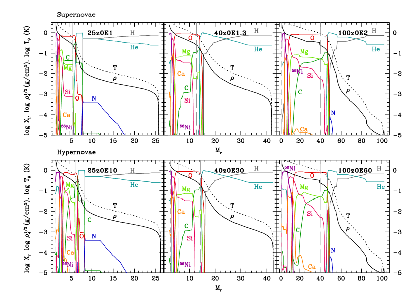
Figure 1.— The density, temperature of zero metallicity presupernovae and composition after explosive nucleosynthesis. The short dashed and long dashed lines correspond to $M_{\rm{cut}}$(ini) and $M_{\rm{mix}}$(out) in mixing-fallback models.

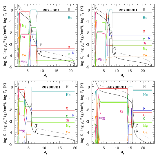
Figure 2.— The density, temperature of non-zero metallicity presupernovae and composition after explosive nucleosynthesis. Mass cut is shown by long dashed line.

The results of our simulations can also be used for finding and identification of low metallicity SNe.

The paper is organized as follows. In section 2 we describe the mixing-fallback models and numerical methods used in calculations. Section 3 presents the results of the calculations of the light curves from the shock breakout epoch to the ⁵⁶Co decay. In Section 4 we make the comparison of the modeling with observed massive type II SNe. Finally, in Section 5 summary and discussion are given.

2. MODELS AND METHODS

2.1. Models

We calculate light curves for zero metallicity progenitors with the main-sequence masses $M_{\rm{MS}}=25,40,100\,$M_⊙ and the explosion energies corresponding to SNe ($E_{\rm{51}}\equiv E/10^{51}$ erg = 1) and hypernovae (HNe)($E_{\rm{51}}\geq$ 10) (see Table 1 for details). The presupernova models include detailed postprocess nucleosynthesis calculations (Tominaga et al., 2007a). The mass loss is considered as a function of metallicity and is supposed to be zero for Pop III models. The composition of the models after explosive nucleosynthesis and density structures of presupernova stars are shown in Figure 1. Presupernova stars with $M_{\rm{MS}}=25,40$ M_⊙ are blue supergiants (BSGs) and these progenitor models have been used by Ishigaki et al. (2014) to find mixing-fallback best-fit models. The transition between red supergiant (RSG) and BSG zero-metallicity stars is still under investigation and we add a RSG progenitor model with $M_{\rm{MS}}=100$ M_⊙ model, RSG progenitor, to give a more complete picture. The fits of the initial mass distribution to the ensemble of inferred Population III star gives $87^{+13}_{-33}$ M_⊙ for the maximum progenitor mass (Fraser et al., 2015), close to our choice of 100 M_⊙ model. For the 100 M_⊙ model we did not find a good mixing-fallback parameters to fit the observed metal poor stars, nevertheless the best models have a small mass of ⁵⁶Ni: $M$(⁵⁶Ni$)\sim 10^{-7}$ M_⊙.

Table 3Zero metallicity supernovae properties

Model	$\Delta t$	$L$	$u_{\rm{ph}}$	$L_{\rm{SBO}}$	$T_{\rm{eff,SBO}}$	$u_{\rm{ph,SBO}}$	log($N_{\rm{UV}}$)
	[days]	[$10^{9}$L⊙]	[$10^{3}$km s-1]	[$10^{9}$L⊙]	[$10^{6}$K]	[$10^{3}$km s-1]	$>13.6$eV
25z0E1	50	0.06	1.5	6	0.3	17	57 (57)
25z0E1m	50	0.06	1.5	8	0.3	17	57 (57)
25z0E10	40	0.3	5	50	0.5	43	59 (58)
25z0E10m	35	0.4	5	50	0.5	43	57 (57)
40z0E1.3m	50	0.1	3	20	0.2	15	57 (57)
40z0E30	35	0.9	7	300	0.4	53	59 (58)
40z0E30m	30	1.0	7	300	0.4	53	59 (58)
40z0E30m2	30	1.2	8	300	0.4	53	59 (58)
100z0E2m	135	1.5	3	30	0.05	3	59 (59)
100z0E60	70	23.3	16	300	0.1	19	60 (60)
100z0E60m	70	34.8	22	300	0.1	19	60 (60)

Note. — The numbers shown are the duration of light curve plateau, the luminosity at the midpoint of the plateau, the photosphere velocity at the mid-plateau epoch, the peak luminosity at shock breakout epoch, photosphere velocity at shock breakout epoch, the number of UV photons in the models with ⁵⁶Ni (in brackets the number of UV photons in the models with $M$(⁵⁶Ni)=0). Plateau characterisics ($\Delta t$, $L$, $u_{\rm{ph}}$) are shown for models with $M$(⁵⁶Ni)=0.

Table 4Non zero metallicity supernovae properties

Model	$\Delta t$	$L$	$u_{\rm{ph}}$	$L_{\rm{SBO}}$	$T_{\rm{eff,SBO}}$	$u_{\rm{ph,SBO}}$	log(${N_{\rm{UV}}}$)
	[days]	[$10^{9}$L⊙]	[$10^{3}$km s-1]	[$10^{9}$L⊙]	[$10^{6}$K]	[$10^{3}$km s-1]	$>13.6$eV
20z-3E1	105	0.47	4	15	0.07	5	58 (58)
20z002E1	115	0.47	4	17	0.07	5	58 (58)
25z002E1	125	0.62	3.5	35	0.07	4	59 (59)
25z002E1m	135	0.74	4	40	0.07	4	59 (59)
40z002E1	80	0.8	4.5	35	0.06	3	59 (59)
40z002E2	70	1.7	9	100	0.08	4	59 (59)

Note. — The numbers shown are the duration of light curve plateau, the luminosity at the midpoint of the plateau, the photosphere velocity at the mid-plateau epoch, the peak luminosity at shock breakout epoch, photosphere velocity at shock breakout epoch, the number of UV photons in the models with ⁵⁶Ni (in brackets the number of UV photons in the models with $M$(⁵⁶Ni)=0). Plateau characterisics ($\Delta t$, $L$, $u_{\rm{ph}}$) are shown for models with $M$(⁵⁶Ni)=0.

The aspherical effects are taken into account with the mixing-fallback model which uses three parameters: the initial mass cut $M_{\rm{cut}}$(ini), the outer boundary $M_{\rm{mix}}$(out) and the ejection factor $f$ (Tominaga et al., 2007b). The parameters of mixing-fallback model are choosen around the values which provide best-fit to the observed elemental abundances (Ishigaki et al., 2014). However, in order to investigate the dependence of light curves on the ejected mass of ⁵⁶Ni, we vary the ejection factor $f$ from the ordinary supernova values $0.07-0.2\,$M_⊙ down to the extremely metal poor case of $M$(⁵⁶Ni$)=10^{-7}\,$M_⊙.

For the 40 and 100 M_⊙ SN models we have to slightly increase the explosion energy from $E_{51}$=1 to 1.3 and 2 correspondingly (see Table 1), in order to avoid the numerical oscillation of internal zones due to the fallback in the spherical symmetric approximation. Thus, the luminosities of these models are higher than those for the originally supposed explosion energy $E_{51}$=1. Estimations for plateau phase (distinctive flat stretch during the decline) gives the increase in 0.3 mag for the 25 M_⊙ model and in 0.7 mag for the 100 M_⊙ model. As the nucleosynthetic products are not influenced much by the small change in the explosion energy, these changes do not lead to any inconsistency. This fallback issue should be investigated in the future with the use of multi-dimensional calculations.

In addition to zero metallicity progenitors we adopt progenitors with various metallicities up to solar (see Figure 2 and Table 2). The solar metallicity models are RSGs, so that the density and temperature inside the H-rich envelope are about several orders of magnitude lower than those of zero metallicity models.

The solar metallicity models undergo mass loss (Figure 2), which is most significant for the 40 M_⊙ model. We do not apply the mixing-fallback scenario for these models using them only for qualitative comparison with zero metallicity models. The mass of the mixing zone usually does not produce a significant changes of light curves. However, in order to investigate mixing effects, we apply mixing-fallback model to both the 25 M_⊙ zero and solar metallicity progenitors.

Similar to zero metallicity models to avoid numerical oscillations we have to slightly change the explosion parameters. We adopt the explosion energy larger than $E_{\rm{51}}=$ 1 for the 40 M_⊙ solar metallicity supernova model 40z002E2 with low mass cut.

2.2. stella code

For calculation of the light curves we use the multigroup radiation hydrodynamics numerical code stella (Blinnikov et al., 1998, 2000, 2006) and for hypernova simulations we include special relativistic corrections in the hydro code in the manner of Misner & Sharp (1969). stella solves implicitly time-dependent equations for the angular moments of intensity averaged over fixed frequency bands and computes variable Eddington factors that fully take into account scattering and redshifts for each frequency group in each mass zone. Here we set $200$ frequency groups in the range from $10^{-3}$ Å  to $5\times 10^{4}$ Å. The explosion is initialized as a thermal bomb just above the mass cut, producing a shock wave that propagates outward. The effect of line opacity is treated as an expansion opacity according to the prescription of Eastman & Pinto (1993) (see also Blinnikov et al. (1998)). The opacity table includes $1.5\times 10^{5}$ spectral lines from Kurucz & Bell (1995) and Verner et al. (1996).

3. RESULTS

The results of the light curves calculations for zero metallicity models are summarized in Table 3, for non-zero metallicity models in Table 4. Below we discribe in details the results of calculations for zero metallicity models at every phases: from shock breakout through the ⁵⁶Co decay. We also highlight the modes reproducing the C-normal EMP ([C/Fe]$\lesssim+1$), CEMP ([C/Fe]$\gtrsim+1$) and HMP ([C/Fe]$\gtrsim+3$) stars and make a comparison with non-zero metallicity SNe.

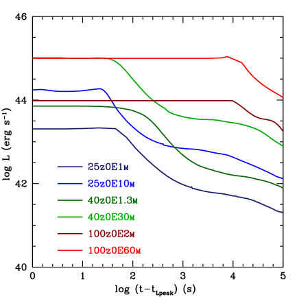
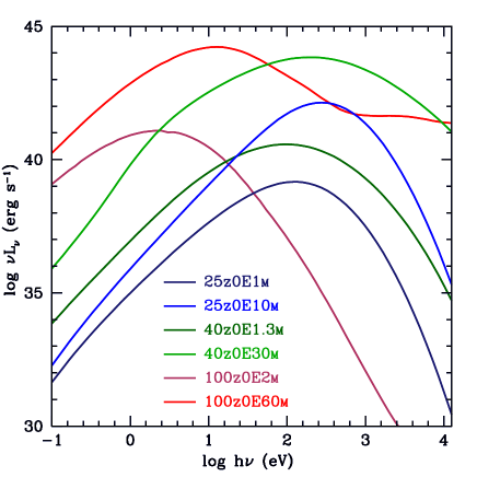
Figure 3.— Bolometric light curves and spectra at shock breakout epoch for zero metallicity models.

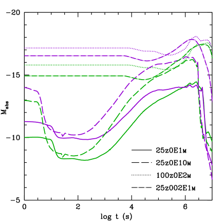
Figure 4.— U-band (violet color) and V-band (green color) light curves for zero and solar metallicity models from shock breakout to plateau phase.

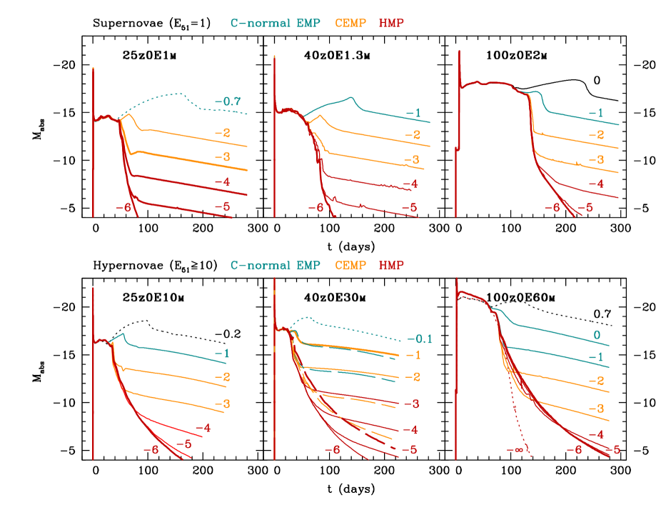
Figure 5.— Bolometric light curves of zero-metallicity SNe parametrized by log($M$(⁵⁶Ni)/M$\odot$) for mixing-fallback models (solid line), original non-mixed models (dotted line) and large mass cut 40z0E30M2 model (dashed line). Solid lines denote the models with the best fit to metal poor stars. Colors denote the EMP (turquoise color), CEMP (orange color) and HMP models (red color).

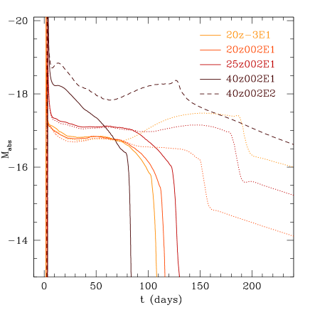
Figure 6.— Bolometric light curves for non-zero metallicity (close to solar metallicity) progenitor models with zero amount of ⁵⁶Ni (solid line) and original non-mixed model (dotted line). Dashed line represents the model 40z002E2. In contrast to the model 40z002E1, 40z002E2 has higher explosion energy $\bm{E_{\rm{51}}=}$ 2, lower mass-cut $\bm{M_{cut}}$=1.5M_⊙ and non-zero nickel mass $\bm{M}$(⁵⁶Ni)=0.7M_⊙.

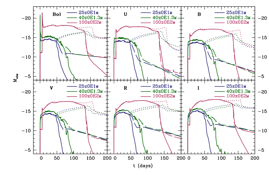
Figure 7.— Bolometric and UBVRI light curves for zero metallicity mixing-fallback supernova models (the explosion energy $E_{51}\sim$ 1). Solid line – $M$(⁵⁶Ni)=0 (HMP), dashed line – $M$(⁵⁶Ni)=$10^{-3}$M_⊙ (CEMP), dotted line – $M$(⁵⁶Ni)=$10^{-1}$M_⊙ (C-normal EMP).

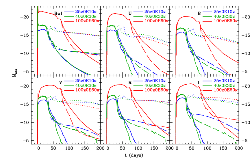
Figure 8.— Bolometric and UBVRI light curves for zero metallicity mixing-fallback hypernova models (the explosion energy $E_{51}\bm{\geq$}10).Solidline--$M$($^56$Ni)=0(HMP),dashedline--$M$($^56$Ni)=$10^-3 $M$_⊙$(CEMP),dottedline--$M$($^56$Ni)=$10^-1 $M$_⊙$(C-normalEMP).$

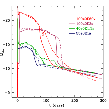
Figure 9.— Bolometric light curves for zero metallicity progenitor models with $M$(⁵⁶Ni)=$10^{-3}$ M_⊙ (solid line) and mixed model (dashed line).

3.1. Shock breakout

In this subsection we mostly describe the properties of zero-metallicity models at the epoch of shock breakout and the difference between zero and solar metallicity models. More detailed investigation of Type II plateau supernova (SN II-P) shock breakout for non zero metallicity progenitors has been done by Tominaga et al. (2011).

The light curves and spectra at the epoch of shock breakout for zero-metallicity models are presented in Figure 3. The duration of the shock breakout are mostly defined by the radius of the progenitors and varies from $\sim$ 100 s for BSGs up to $\sim$ 1000 s for RSGs. The peak frequency of BSG models (25,40 M_⊙) is in X-ray and their shock breakout can be detected for example by SWIFT/XRT telescope up to $z\sim 0.1$ for SN and $z\sim 1$ for HN models.

The shape of the spectrum for the 100 M_⊙ hypernova model is different from the others because of several density peaks in the outer layers of the ejecta. These peaks are formed due to inefficient gas acceleration (Tolstov et al., 2013) and for such cases more reliable calculations can be done only in multidimensional consideration of fragmentation in the outer layer.

The shock breakout phase of solar metallicity supernovae has larger luminosity, but the effective temperature is much lower for the same mass in comparison with zero metallicity supernovae (see Table 4). The main properties of shock breakouts depend on the radius, the ejecta mass, the explosion energy, the opacity and the density structure of the external layers (see, e.g., analityc estimations of Imshennik & Nadezhin, 1988; Matzner & McKee, 1999). The dependence of the duration of the shock breakout $\Delta t_{SBO}$ and the peak luminosity $L_{SBO}$ on presupernova parameters can be estimated as follows (Matzner & McKee, 1999):

$$\Delta t_{SBO}=790\Big{(}\frac{\kappa}{0.34\rm{cm}^{2}\rm{g}^{-1}}\Big{)}^{-0.58}\Big{(}\frac{E}{10^{51}\rm{erg}}\Big{)}^{-0.79}$$

$$\times\Big{(}\frac{\rho_{1}}{\rho_{*}}\Big{)}^{-0.28}\Big{(}\frac{M}{10\rm{M}_{\odot}}\Big{)}^{0.21}\Big{(}\frac{R}{500\rm{R}_{\odot}}\Big{)}^{-0.79}\,\rm{s}\,\,\rm{(RSG)}\,,$$

$$\Delta t_{SBO}=40\Big{(}\frac{\kappa}{0.34\rm{cm}^{2}\rm{g}^{-1}}\Big{)}^{-0.45}\Big{(}\frac{E}{10^{51}\rm{erg}}\Big{)}^{-0.72}$$

$$\times\Big{(}\frac{\rho_{1}}{\rho_{*}}\Big{)}^{-0.18}\Big{(}\frac{M}{10\rm{M}_{\odot}}\Big{)}^{0.27}\Big{(}\frac{R}{50\rm{R}_{\odot}}\Big{)}^{1.90}\,\rm{s}\,\,\rm{(BSG)}\,,$$ (1)

$$L_{SBO}=2.2\cdot 10^{45}\Big{(}\frac{\kappa}{0.34\rm{cm}^{2}\rm{g}^{-1}}\Big{)}^{-0.29}\Big{(}\frac{E}{10^{51}\rm{erg}}\Big{)}^{1.35}$$

$$\times\Big{(}\frac{\rho_{1}}{\rho_{*}}\Big{)}^{-0.37}\Big{(}\frac{M}{10\rm{M}_{\odot}}\Big{)}^{-0.65}\Big{(}\frac{R}{500\rm{R}_{\odot}}\Big{)}^{-0.42}\,\rm{erg\,s^{-1}}\,\,\rm{(RSG)}\,,$$

$$L_{SBO}=1.9\cdot 10^{45}\Big{(}\frac{\kappa}{0.34\rm{cm}^{2}\rm{g}^{-1}}\Big{)}^{-0.39}$$

$$\quad\quad\times\Big{(}\frac{E}{10^{51}\rm{erg}}\Big{)}^{1.30}\Big{(}\frac{\rho_{1}}{\rho_{*}}\Big{)}^{-0.23}$$

$$\quad\quad\times\Big{(}\frac{M}{10\rm{M}_{\odot}}\Big{)}^{-0.69}\Big{(}\frac{R}{50\rm{R}_{\odot}}\Big{)}^{-0.22}\,\rm{erg\,s^{-1}}\,\,\rm{(BSG)}\,,$$ (2)

where $\kappa,E,M$ and $R$ are the opacity, the explosion energy, the mass of the ejecta and the radius of the presupernova, respectively. The density factor $\rho_{1}/\rho_{*}\approx 1$ for RSG models. For BSGs $\rho_{1}/\rho_{*}$ depends on the density structure, composition and luminosity of the outer layers of the star and varies from $\rho_{1}/\rho_{*}\approx 50$ for the 25 M_⊙ model to $\rho_{1}/\rho_{*}\approx 2$ for the 40 M_⊙ model.

The difference between RSG and BSG models are clearly seen by the duration of the peak: the larger presupernova radius leads to a longer duration of the shock breakout epoch. In comparison with zero metallicity BSGs, the larger luminosity of solar metallicity SNe is due to lower (by several orders of magnitude) opacity of the external layers of RSG. The photosphere’s temperature of RSG models is only 3,000-4,000 K (in contrast to $\sim$ 20,000 K in BSG models) and the opacity of neutral atoms of hydrogen is dominated by bound-bound and bound-free transitions. In accordance with theoretical estimations this low opacity of exteral layers increases the luminosity of the shock breakout.

3.2. Cooling phase and rising time

The shock breakout is followed by "cooling envelope phase" the decline of the luminosity (see Figure 4). The duration of this phase strongly depends on the presupernova radius. For compact BSG progenitors the duration is much shorter in optical U and V bands ($\sim$ 100 s) than for RSGs ($\sim$ 1 day). After reaching the luminosity minimum, the light curve starts rising, as the heated expanding stellar envelope diffuses out. For RSG progenitors the rise-time ($\sim$ 10 days) is the order of magnitude longer than for BSG progenitors. This behavior is consistent with the previous investigation of the SN light curves for the early phases (see, e.g., González-Gaitán et al., 2015).

3.3. Plateau phase

The presence of the massive hydrogen envelope in zero metalicity presupernova models should produce light curve similar to SNe II-P. The duration of the plateau is determined primarily by the mass of the envelope $M_{\rm{ej}}$ and the other main outburst properties, the explosion energy $E$ and the initial radius $R$ (Litvinova & Nadezhin, 1985; Popov, 1993). The SN II-P light curve tails are believed to be powered by the ⁵⁶Co decay and the temporal behavior is determined by the ejected mass of ⁵⁶Ni (see, e.g., Nadyozhin, 1994). The variation of the ejected mass of ⁵⁶Ni allows to cover the uncertainty of matter mixing and fallback in aspherical, jet-like explosion. We start with $M$(⁵⁶Ni) $\sim$ $0.1$M_⊙ and logarithmically decrease down to $10^{-6}$M_⊙ by a factor of $10$M_⊙. Lower values of $M$(⁵⁶Ni) leads to extremely small changes in the light curve ($M_{\rm{abs}}<-5$) and for practical purposes the light curve with $M$(⁵⁶Ni)=$10^{-6}$M_⊙ can be used. The light curves for zero-metallicity models are compared with several RSG models with zero amount of ⁵⁶Ni.

3.3.1 Plateau luminosity

During the plateau the light curve is powered by shock conversation of the kinetic energy into the thermal energy during the shock propagation in the stellar envelope. The peak luminosity increases with higher explosion energy and radius, but decreases with higher ejecta mass. The absolute V magnitude can be estimated from Litvinova & Nadezhin (1985):

$$V=-2.34\lg E-1.80\lg R+1.22\lg M-11.307\,,$$ (3)

where $E,R,$ and $M$ are the explosion energy (in 10⁵⁰ erg), the presupernova radius and the ejecta mass in solar units, respectively.

The calculations of zero metallicity models presented in Figure 5 are consistent with the analytic estimations. The plateau of the 25 M_⊙ and 40 M_⊙ supernovae having compact progenitor is rather faint: $M_{\rm{bol}}\sim$ -15, while much larger radius of 100 M_⊙ progenitor leads to the increase of luminosity. In contrast to the zero metallicity 25-40 M_⊙ models, solar metallicity SNe are about an order of magnitude more luminous (Figure 6) due to larger radius of the progenitors.

All the above are valid for the models with low amount of ⁵⁶Ni. If the ⁵⁶Ni mass in the ejecta is rather high ($M$(⁵⁶Ni)$>$ 0.01…1M_⊙), the ⁵⁶Ni decay can form more luminous peak. From Figure 5 we see that ⁵⁶Ni peak is a possible indicator C-normal EMP stars.

The optical multicolor light curves (Figures 7-3) during the plateau phase demonstrate that the flat shape of the U and B band light curves is similar to the bolometric light curve. The shape of the light curves in more luminous R and I bands is not so flat and has a peak in the middle of the plateau.

3.3.2 Plateau duration

The duration $\Delta t$ of the light-curve plateau is estimated by Litvinova & Nadezhin (1985) as:

$$\Delta t=-0.191\lg E+0.186\lg R+0.566\lg M+1.047\,.$$ (4)

In accordance with this equation, the larger radius and mass provide longer duration of the plateau phase, but larger explosion energy reduces the plateau duration. This behavior is well reproduced in our numerical calculations: in bolometric light curves of zero metallicity (Figure 5) and solar metallicity (Figure 6) models and in multicolor light curves of zero metallicity supernova and hypernova models (Figures 7-3).

The width of the plateau depends also on the depth of the mixed hydrogen-rich layer (see, e.g., Shigeyama & Nomoto, 1990). To estimate the influence of mixing we constructed models with uniform abundances distribution and made a comparison with non-mixed models (Figure 9). The mixing does not greatly change the form of the light curve because the minimum velocity of the hydrogen layer is low for the models.

The solar metallicity RSG progenitor has larger radius which leads to higher luminosity and longer duration of the SN plateau in comparison with BSG progenitors. The 20 M_⊙ and 25 M_⊙ RSG models have quite a large amount of ⁵⁶Ni to make the plateau duration longer in comparison with the low-⁵⁶Ni models (Figure 6).

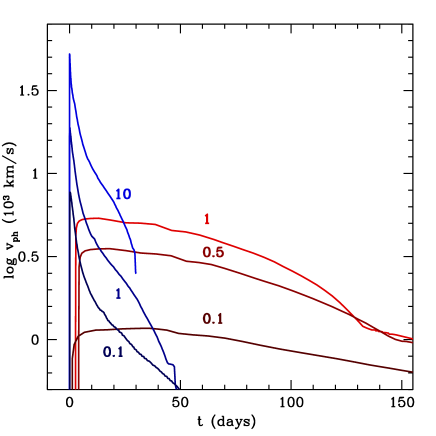
Figure 10.— Photosperic velocities for 25 M_⊙ zero metallicity (blue color) and solar metallicity (red color) progenitors with $M$(⁵⁶Ni)=0, parametrized by the explosion energy $E_{51}$.

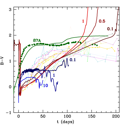
Figure 11.— Calculated $B-V$ color evolution curves (mag) of 25 M_⊙ zero-metallicity progenitors (solid blue lines) with $M$(⁵⁶Ni)=0, solar metallicity progenitors (solid red lines) with $M$(⁵⁶Ni)=0, parametrized by the explosion energy ($E_{51}$=0.1;0.5;1;10) and SN1987A (solid green line). Green dots denote SN 1987A observed $B-V$ color evolution curve (Hamuy & Suntzeff, 1990), light color lines - the observational data for a set of 16 SN II-P (Hamuy, 2001). For calculation of SN1987A color curve (green line) the results of Blinnikov et al. (2000) are used.

Figure 12.— V-band light curves for 25 M_⊙ solar metallicity progenitors with the explosion energy $E_{51}$=0.1;1 (solid brown and red lines), and their comparison with V-band light curves for 25 M_⊙ ($\bm{E_{51}}$=1) and 100 M_⊙ ($\bm{E_{51}}$=2) zero metallicity progenitors (dashed blue and maroon colors). Light curve of 25 M_⊙ zero metallicity model is shifted by 160 days from the moment of explosion. For all the models $\bm{M}$(⁵⁶Ni)=0.

3.3.3 Photospheric velocities

In Figure 10 we compare the photosperic velosities for 25 M_⊙ zero and solar metallicity models during plateau phase. Due to compact presupernova, zero metallicity model have higher velocity and much faster drop of the photospheric velocity. For hypernova models (explosion energy $E_{51}$=10) the velocity of the outer layers of the ejecta reaches $\sim$ 50,000 km s^-1. The modeling of the color The maximum photospheric velocity is realized at the beginning of the plateau phase just after shock breakout epoch.

3.3.4 Color evolution curves

Figure 11 presents $B-V$ color evolution curves of 25 M_⊙ progenitors for various values of explosion energy and metallicity. The color evolution curves reveal the common feature: for zero and low metallicity BSG progenitors the $B-V$ value during plateau phase is almost constant, while for solar metallicity RSG progenitors we can see a gradual reddening.

For more general investigation, in Figure 11 we compare the color evolution curves calculated by stella with a set of SN II-P and SN1987A observational data. The modeling of the color evolution curves during the plateau phase demonstrates the cooling rate consistent with observed SNe: the decrease of metallicity leads to flattening of the color evolution curve. The flattening of the color curve also can be seen in observations of low metallicity supernovae (see, e.g., Polshaw et al., 2015).

It is difficult to use the luminosity and the duration of the plateau phase to distinguish between solar and low metallicity SNe (Figure 12). Zero metallicity normal energy SNe are as luminous as solar metallicity low energy SNe. Moreover, the light curve of the massive 100 M_⊙ zero metallicity SN is quite similar (in the plateau duration and luminosity) to the light curve of less massive (25 M_⊙) solar metallicity star for the same explosion energy $E_{51}$ = 1. The decline of the luminosity after the plateau phase is also quite similar between the zero and solar metallicity progenitors (Figure 12). In this situation the SN color evolution curve can help to distinguish the metallicity of the progenitor.

In Figure 13 we compare the color evolution curves for zero and solar metallicity RSG models and find that they also differ in the cooling rate and, consequently, can be distinguished in metallicity. For massive zero metallicity BSG presupernova model (40z0E1.3), in contrast to RSGs, the plateau is shorter, but again low metallicity leads to the flattening of the color evolution curve.

In addition, we confirm the above metallicity dependence with 100 M_⊙ models in which the metallicity of hydrogen envelope changes gradually from zero to the solar value. The result of this numerical experiment is the same as above: for zero metallicity model $B-V$ and $U-B$ color evolution curve are flat, but the increase of metallicity to the solar value leads to the linear behavior. The color evolution is mostly due to opacity difference between zero and solar metallicity models, while hydrodynamical evolution for both models is similar. In distinguishing between zero and solar metallicity models, the evolution of red and infrared color indexes is less informative in comparison with $B-V$ color index.

The different behaviour of low metallicity and solar metallicity color evolution curves can be used to distinguish low metallicity and normal metallicity SNe.

Figure 13.— Calculated $B-V$ color evolution curves (mag) during plateau phase of 25 M_⊙ solar metallicity RSG progenitor (solid red line) with the explosion energy $\bm{E_{51}}$=1, 40 M_⊙ zero metallicity BSG progenitor (dotted green line) ($\bm{E_{51}}$=1) and 100 M_⊙ zero metallicity RSG progenitor (dashed maroon line) ($\bm{E_{51}}$=2). For all the models $\bm{M}$(⁵⁶Ni)=0.

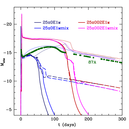
Figure 14.— Bolometric light curves for zero and solar metallicity mixing-fallback 25 M_⊙ supernova models (the explosion energy $E_{51}$ = 1). Blue and magenta colors denote the models with uniform mixing throughout the ejecta. Solid line – $M$(⁵⁶Ni)=0 (HMP), dashed line – $M$(⁵⁶Ni)=$10^{-3}$ M_⊙ (CEMP), dotted line – $M$(⁵⁶Ni)=$10^{-1}$ M_⊙ (EMP). The green dots denote bolometric light curve of SN 1987A with $M$(⁵⁶Ni)=0.07 M_⊙ (Suntzeff & Bouchet, 1990)

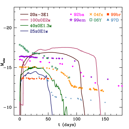
Figure 15.— V-band light curves for zero metallicity (red, green, blue colors), non-zero metallicity (dark red color) and a number of observed SNe. For all the models $\bm{M}$(⁵⁶Ni)=0.

3.4. Transition from plateau to ⁵⁶Co decay

After the plateau phase for low ⁵⁶Ni models the luminosity starts to decline. The decline rate is defined by the explosion energy (Arnett, 1980), opacity, ⁵⁶Ni and H mixing (see, e.g., Kasen & Woosley, 2009; Bersten et al., 2011; Nakar et al., 2015).

UBVRI light curves for low ⁵⁶Ni models are summarized in Figure 7-3. The radius of BSGs is smaller in comparison with RSGs and the temperature drops faster (Grasberg et al., 1971; Arnett, 1980). This leads to the steeper luminosity decline in optical bands for BSG models.

The presence of ⁵⁶Ni finally leads to the tail of the light curve powered by the ⁵⁶Co decay and its temporal behaviour is given by (see, e.g., Nadyozhin, 1994):

$$M_{\rm{bol}}=-19.19-2.5\lg{\Big{(}\frac{M_{\rm{Ni0}}}{M_{\odot}}\Big{)}}-1.09\frac{t}{\tau_{\rm{Co}}}\,,$$ (5)

where $t$ is measured from the moment of explosion ($t=0$), $M_{\rm{Ni0}}$ is the total mass of ⁵⁶Ni at $t=0$ which decays with a half-life of 6.1 days into ⁵⁶Co, and $\tau_{\rm{Co}}$=111.3 days.

The smooth radioactive tail is reproduced in all our numerical calculations with good accuracy.

If we increase ⁵⁶Ni mass from zero in the model, the radioactive tail becomes more luminous and at some $M$(⁵⁶Ni) mass value its luminosity at the end of the plateau phase can be comparable with the plateau luminosity. This value can be roughly estimated using equations (3-5), and for our models varies from $\sim$ 0.1-0.01 M_⊙ for SNe to $\sim$ 0.1-0.5 M_⊙ for HNe. For these values the nickel peak can be clearly seen in the light curve.

In comparison with zero metallicity SNe models, for solar metallicity models the brightness of the plateau phase is larger and the mass of ⁵⁶Ni for forming the nickel peak is larger: $\gtrsim$ 0.1 M_⊙.

In Figure 3 we find that the luminosity of the most luminous model 100z0E60m without ⁵⁶Ni is higher than for the model with $\bm{M}$(⁵⁶Ni)=$\bm{10^{-3}}$M_⊙ in the transition from plateau to the ⁵⁶Ni tail up to $\sim$ 150 days. This behavior is explained by the trapping of thermal photons in the model with ⁵⁶Ni where the transparency is lower (due to a larger amount of ⁵⁶Fe produced by ⁵⁶Ni and ⁵⁶Co decays). It takes place until the epoch when radioactive decay overwhelms the emission of thermal photons from the entropy reservoir of the shock heated ejecta of zero ⁵⁶Ni model at t $>$ 150 days. Although further, more detailed, study may have some sense to clarify fully the nature of this effect, it is not important for the goals of our investigation. The behavior of light curves in those epochs does not change our conclusions.

3.4.1 Mixing

The above estimations for the transition phase do not take mixing into consideration, but account for mixing can significantly change the light curve.

To investigate the mixing effect more accurately we compare a number of 25 M_⊙ models with zero and solar metallicity, varying $M$(⁵⁶Ni) and calculating light curves for all these models with uniform mixing throughout the ejecta (Figure 14). If $M$(⁵⁶Ni) is rather large ($\gtrsim$ 0.1 M_⊙) the mixing reduces rise time to the ⁵⁶Ni peak (model 25z0E1m). For more plateau luminous models the mixing slightly reduce the plateau duration for the same reason: the ⁵⁶Ni peak is shifted to early times (model 25z002E1m).

3.5. Comparison with previous calculations

We compare the simulation of the multiband light curves of the 25 M_⊙ hypernova model ($E_{\rm{51}}$ = 10) with light curves calculated by Smidt et al. (2014) for similar models. The luminosity of the plateau and its duration are in good agreement with their calculations. The decline of the light curves after the plateau phase is more sloping in stella calculation, which is related to different procedures in opacity calculations. The luminosity at the tail phase must be specified in the future in more detailed opacity calculations that include millions of lines, similar to existing procedures for type Ia SNe (private communication with E. Sorokina). Detailed opacity calculations and the analysis of the transition phase (from the plateau to ⁵⁶Co decay) in the models with $M$(⁵⁶Ni) can help to reveal the physical properties of the presupernova: explosion energy, mixing and opacity.

4. Observational properties of Pop III and metal-poor core-collapse supernovae

4.1. Comparison with the nearby supernovae

In Figure 15 the calculated low-⁵⁶Ni light curves are qualitatively compared with several observed massive Type II SNe (SN 1999em (Elmhamdi et al., 2003), SN 1999br (Pastorello et al., 2004), SN 1997D (Benetti et al., 2001), SN 2004fx (Hamuy et al., 2006), SN 1992ba, SN 2006Y (Anderson et al., 2014)).

The luminosity of the plateau for the observed faint supernova SN 1997D is close to the modelled light curves of SNe having BSG progenitors. Adjusted for the uncertainty of the observed plateau duration and possible asymmetry features, our BSG models with low metallicity could be good candidates for simulation of these object in addition to already existing simulations (Turatto et al., 1998; Chugai & Utrobin, 2000).

The B-V color evolution curves of SN 1999em and SN 1999br are included in the set of SN II-P data (Hamuy, 2001) presented in Figure 11. Their color curves are typical to solar metallicity progenitors and the presupernovae of SN 1999em and SN 1999br are supposed to have RSG progenitors. The B-V color evolution curve for SN 1992ba and SN 2004fx are also typical to solar metallicity SNe (Jones et al., 2009; Hamuy et al., 2006).

Since we do not know the moment of explosion in observed SN II-P, it is difficult to distinguish between the low energy explosion of RSG ($E_{51}\sim$ 0.1) and the ordinary BSG SN in the analysis of bolometric light curves (see Figure 12). The analysis of photosperic velocities and color curve evolution during the plateau phase can provide more information about the progenitor.

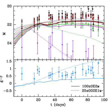
Figure 16.— Optical SDSS ugriz light curves (upper panel) colour-coded violet, green, red, dark red and black respectively, and color evolution curve (lower panel) for SNII (SDSS ID 12991). Observations are compared with zero metallicity 100z0E2m model (solid line) and solar metallicity 25z002E1m model (dashed line). For all the models $\bm{M}$(⁵⁶Ni)=0.

Figure 17.— V-band light curves for zero metallicity (red, green and blue colors) supernovae with $M$(⁵⁶Ni)=0. Horizontal lines represents the Gaia servey detection limits. The dots denote the SN 1987A data of Hamuy & Suntzeff (1990).

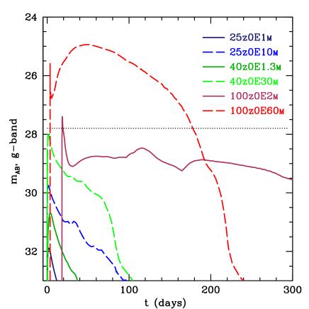
Figure 18.— Apparent g-band light curves for zero metallicity models at redshift z=2. No extinction and no IGM absorption are assumed. The horizontal line shows a 5$\sigma$ detection limit in the g-band for the Subaru/HSC 1 hr integration. For all the models $\bm{M}$(⁵⁶Ni)=0.

4.2. Detectability of Pop III supernovae

While Pop III SNe have typically fainter and shorter plateau than SNe with solar metallicity, the most important characteristics is the color evolution curves. The color evolutions at the plateau phase and at the first $10$ days distinguish the Pop III SNe from RSG SNe with solar metallicity and SN 1987A-like BSG SNe, respectively (Figure 13). In order to obtain the color evolution, the multicolor observations should be performed every $\sim 2$ days for the first $10$ days and every $\sim 10$ days for the plateau.

Although the follow-up observations of nearby SNe realize such multicolor observations with cadences of $<10$ days, SNe with the flat color evolution have not been discovered (Section 4.1). This might be because most of previous SN surveys targeted large nearby galaxies with metal enrichment. Untargeted multicolor SN surveys were performed by SDSS (Sako et al., 2014) and SNLS (Astier et al., 2006; Guy et al., 2010). Their cadences are high enough to draw the color evolution curves at the plateau. We have checked the multicolor light curves of the SDSS sample. Although the signal-to-noise ratio is poor, an SN II spectroscopically identified (ID 12991) shows blue color and flat color evolution curves at the plateau phase (Figure 16). Although the metallicity of host galaxy is not metal-poor according to $R_{23}$ method ($12+\log({\rm O/H})=8.58$, (Tremonti et al., 2004; Alam et al., 2015)), we propose that the SN took place at the low-metallicity environment. We do not consider red and infrared color evolution curves because it is not informative to distinguish zero and solar metallicity (see Section 3.3.4).

There are two directions to detect Pop III SNe in low metallicity environment that produce C-normal EMP, CEMP, and HMP stars. In order to identify low-⁵⁶Ni SNe, it is required to follow the light curve until the ⁵⁶Co decay. As the tail of faint SNe for the HMP stars is as faint as $M_{\rm abs}>-7$, the tail can be detected only if they take place at $<50$ Mpc even with $8$m-class telescopes. In contrast, their plateau are as bright as $m_{\rm bol}\sim 20$ and thus the detection can be made with an untargeted survey with such $1$m-class telescopes as PTF (Rau et al., 2009), KISS (Morokuma et al., 2014) and the all-sky survey as Gaia with the broad-band G band limiting magnitude of $G\sim 19$ (Altavilla et al. 2012). In Figure 17 we plot light curves for low-⁵⁶Ni models and designate the detection limits for Gaia mission. For these surveys, EMP star forming galaxies also can be a good target for finding and identification of supernovae of metal-poor progenitor stars (Pilyugin et al., 2014; Thuan, 2008; Guseva et al., 2015)

The other targets to detect Pop III SNe are the metal-free pockets at $z\sim 2$. Figure 18 shows the $g$-band light curves of Pop III SNe at $z=2$. Since Pop III SNe are fainter than SNe with solar metallicity, only the SNe with $100~{}$M_⊙ can be observed with such $8$m-class telescopes as Subaru/HSC and LSST. The explosions with $E_{51}=1$ and $60$ can be detected at the shock breakout phase and the phase from the shock breakout to the plateau, respectively. The UV color of Pop III SNe also display the flat color evolution, in contrast to the increasing UV color evolution of solar metallicity SNe (Figure 19). Therefore, the multicolor optical observation can inform the metallicity of the SN, although the spectroscopic follow-up observation is difficult.

4.3. Contribution to the ionization

The sources of UV radiation capable to reionize the Universe are still under discussion. According to cosmological models (Barkana & Loeb, 2001) and observations (Fan et al. (2006)) the reionization of the Universe appears to have well completed at redshift $z\sim 6$. The first generation stars could be the imporant contributors to the ionization. According to our calculations SNe of RSG progenitors provide larger amount of UV photons at the shock breakout epoch, but still less than BSGs do during lifetime.

To estimate the contribution of Pop III SNe to cosmic reionization we calculate the number of ionizing photons with the energy $E_{\rm{ion}}=h\nu_{\rm{HI}}>13.6$ eV for all the models:

$$N_{\rm{UV}}=\int_{\nu_{\rm{HI}}}^{\infty}\frac{F_{\nu}}{h\nu}d\nu$$ (6)

The results are summarized in the last column of Table 3. The UV photons are mostly produced by shock breakout when the effective temperature is high enough ($T\sim 5\times 10^{5}$ K), being similar to previous estimations from the SN 1987A model (Lundqvist & Fransson, 1996). Supernovae with larger explosion energies or larger progenitor radii emit larger number of UV photons. But for BSG progenitors the number of UV photons during explosions corresponds only 10 – 100 yr of the main-sequence lifetime(Tumlinson & Shull, 2000). RSG progenitors provides a larger amount of UV photons at shock breakout, but still less than those from BSGs during lifetime.

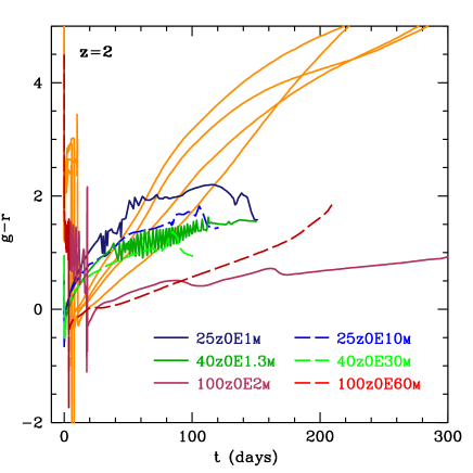
Figure 19.— Color evolution light curves at redshift z=2 during plateau phase for solar metallicity (orange color) and zero metallicity (blue color - 25 M_⊙, green color - 40 M_⊙ and red color - 100 M_⊙) models. SN models (solid line) and HN models (dashed line) are presented. No extinction and no IGM absorption are assumed. For all the models $\bm{M}$(⁵⁶Ni)=0.

5. CONCLUSIONS

We have calculated the light curves for a number of hydrodynamical models for Pop III 25 – 100 M_⊙ core-collapse SNe ($E_{51}\sim$ 1) and HNe ($E_{51}\sim$ 10). These models are assumed to undergo mixing and fallback to produce nucleosynthesis yields being well fitted to the observed abundance patterns of EMP, HMP, and CEMP stars.

The radiation-hydrodynamical simulations reproduce in details shock breakout, plateau phase and radioactive tail of the light curves. The observations of shock breakout and multicolor light curves of the plateau phase is important for the identification of zero and low metallicity SNe.

BSGs are typical presupernova for Pop III core collapse SNe with $M\lesssim$ 40-60 M_⊙ and their structure determine the properties of shock breakout: shorter duration and lower luminosity in comparison with more massive RSG progenitors. The plateau phase is common to both BSG and RSG models and can provide the information that the progenitors are similar to SN II-P. But the duration of the plateau phase is often unknown from the observation. The evolution of photospere’s velocity and multiband light curves can be more useful for the identification of Pop III SNe. We have found that the flat color evolution curve $B-V$ during plateau phase can be used as an indicator of low-metallicity SNe.

The low amount of ⁵⁶Ni to explain CEMP stars with mixing-fallback leads to a sharp luminosity decline after the plateau phase. This feature also can be used as an indicator of low metallicity progenitor. The transition phase from the plateau to the tail can give us the additional information about the explosion energy, mixing and opacity of the presupernova, but it requires more accurate theoretical consideration of opacities in numerical simulations.

We have modelled Pop III SNe with 1D simulations. The aspherical effects are taken into account approximately with the mixing-fallback model. The mixing of H and ⁵⁶Ni could have a large impact on the shape of the light curve and future multi-dimensional radiation calculations are preferred to investigate the effects of asphericity more accurately.

The direct detection of Pop III core-collapse SNe is hardly possible at high redshift (Whalen et al., 2013), but Pop III hypernovae will be visible to the JWST (James Webb Space Telescope) at z $\,\sim\,$ 10 – 15 (Smidt et al., 2014). The probability of the detection iof Pop III SNe in metal-free gas pockets (z $\,\sim\,$ 2) would be higher, where the detection would be possible by current surveys (HSC/Subaru).

Along with Pop III SNe the results our modeling would be suitable for identification of low-metallicity supernovae in the nearby Universe. The BSG progenitors are supposed to have the metallicity up to Z $\,\sim\,$ 10^-5 – 10^-4. There is a number of galaxies in the local Universe with metallicities close to these values (Papaderos et al., 2008; Pilyugin et al., 2014) and with account of inhomogeneous galaxy regions there would be a good chance for identification and study of these objects. The number of discovered faint supernovae is increasing (Nomoto, 2012) and the new surveys LSST, JWST (James Webb Space Telescope) are planned to make a large contribution to the detection of low metallicity supernovae.

References

- Alam et al. (2015) Alam, S., Albareti, F. D., Allende Prieto, C., et al. 2015, ApJS, 219, 12
- Anderson et al. (2014) Anderson, J. P., González-Gaitán, S., Hamuy, M., et al. 2014, ApJ, 786, 67
- Aoki et al. (2014) Aoki, W., Tominaga, N., Beers, T. C., Honda, S., & Lee, Y. S. 2014, Science, 345, 912
- Arnett (1980) Arnett, W. D. 1980, ApJ, 237, 541
- Astier et al. (2006) Astier, P., Guy, J., Regnault, N., et al. 2006, A&A, 447, 31
- Barkana & Loeb (2001) Barkana, R., & Loeb, A. 2001, Phys. Rep., 349, 125
- Beers & Christlieb (2005) Beers, T. C., & Christlieb, N. 2005, ARA&A, 43, 531
- Benetti et al. (2001) Benetti, S., Turatto, M., Balberg, S., et al. 2001, MNRAS, 322, 361
- Bersten et al. (2011) Bersten, M. C., Benvenuto, O., & Hamuy, M. 2011, ApJ, 729, 61
- Blinnikov et al. (2000) Blinnikov, S., Lundqvist, P., Bartunov, O., Nomoto, K., & Iwamoto, K. 2000, ApJ, 532, 1132
- Blinnikov et al. (1998) Blinnikov, S. I., Eastman, R., Bartunov, O. S., Popolitov, V. A., & Woosley, S. E. 1998, ApJ, 496, 454
- Blinnikov et al. (2006) Blinnikov, S. I., Röpke, F. K., Sorokina, E. I., et al. 2006, A&A, 453, 229
- Bromm & Yoshida (2011) Bromm, V., & Yoshida, N. 2011, ARA&A, 49, 373
- Cayrel et al. (2004) Cayrel, R., Depagne, E., Spite, M., et al. 2004, A&A, 416, 1117
- Chugai & Utrobin (2000) Chugai, N. N., & Utrobin, V. P. 2000, A&A, 354, 557
- Crighton et al. (2015) Crighton, N. H. M., O’Meara, J. M., & Murphy, M. T. 2015, ArXiv e-prints, arXiv:1512.00477
- Drake et al. (2009) Drake, A. J., Djorgovski, S. G., Mahabal, A., et al. 2009, ApJ, 696, 870
- Eastman & Pinto (1993) Eastman, R. G., & Pinto, P. A. 1993, ApJ, 412, 731
- Elmhamdi et al. (2003) Elmhamdi, A., Danziger, I. J., Chugai, N., et al. 2003, MNRAS, 338, 939
- Fan et al. (2006) Fan, X., Strauss, M. A., Becker, R. H., et al. 2006, AJ, 132, 117
- Fraser et al. (2015) Fraser, M., Casey, A. R., Gilmore, G., Heger, A., & Chan, C. 2015, ArXiv e-prints, arXiv:1511.03428 [astro-ph.SR]
- Fumagalli et al. (2011) Fumagalli, M., O’Meara, J. M., & Prochaska, J. X. 2011, Science, 334, 1245
- González-Gaitán et al. (2015) González-Gaitán, S., Tominaga, N., Molina, J., et al. 2015, MNRAS, 451, 2212
- Grasberg et al. (1971) Grasberg, E. K., Imshenik, V. S., & Nadyozhin, D. K. 1971, Ap&SS, 10, 3
- Guseva et al. (2015) Guseva, N. G., Izotov, Y. I., Fricke, K. J., & Henkel, C. 2015, A&A, 579, A11
- Guy et al. (2010) Guy, J., Sullivan, M., Conley, A., et al. 2010, A&A, 523, A7
- Hamuy & Suntzeff (1990) Hamuy, M., & Suntzeff, N. B. 1990, AJ, 99, 1146
- Hamuy et al. (2006) Hamuy, M., Folatelli, G., Morrell, N. I., et al. 2006, PASP, 118, 2
- Hamuy (2001) Hamuy, M. A. 2001, PhD thesis, The University of Arizona
- Hansen et al. (2014) Hansen, T., Hansen, C. J., Christlieb, N., et al. 2014, ApJ, 787, 162
- Heger & Woosley (2010) Heger, A., & Woosley, S. E. 2010, ApJ, 724, 341
- Hirano et al. (2014) Hirano, S., Hosokawa, T., Yoshida, N., et al. 2014, ApJ, 781, 60
- Imshennik & Nadezhin (1988) Imshennik, V. S., & Nadezhin, D. K. 1988, Soviet Astronomy Letters, 14, 449
- Ishigaki et al. (2014) Ishigaki, M. N., Tominaga, N., Kobayashi, C., & Nomoto, K. 2014, ApJ, 792, L32
- Iwamoto et al. (2005) Iwamoto, N., Umeda, H., Tominaga, N., Nomoto, K., & Maeda, K. 2005, Science, 309, 451
- Jones et al. (2009) Jones, M. I., Hamuy, M., Lira, P., et al. 2009, ApJ, 696, 1176
- Kasen & Woosley (2009) Kasen, D., & Woosley, S. E. 2009, ApJ, 703, 2205
- Kurucz & Bell (1995) Kurucz, R. L., & Bell, B. 1995, Atomic line list
- Limongi et al. (2003) Limongi, M., Chieffi, A., & Bonifacio, P. 2003, ApJ, 594, L123
- Litvinova & Nadezhin (1985) Litvinova, I. Y., & Nadezhin, D. K. 1985, Soviet Astronomy Letters, 11, 145
- Lucatello et al. (2005) Lucatello, S., Tsangarides, S., Beers, T. C., et al. 2005, ApJ, 625, 825
- Lugaro et al. (2012) Lugaro, M., Karakas, A. I., Stancliffe, R. J., & Rijs, C. 2012, ApJ, 747, 2
- Lundqvist & Fransson (1996) Lundqvist, P., & Fransson, C. 1996, ApJ, 464, 924
- Matzner & McKee (1999) Matzner, C. D., & McKee, C. F. 1999, ApJ, 510, 379
- Misner & Sharp (1969) Misner, C. W., & Sharp, D. H. 1969, in Quasars and high-energy astronomy, Proceedings of the 2nd Texas Symposium on Relativistic Astrophysics, held in Austin, December 15-19, 1964 Edited by K.N. Douglas, I. Robinson, A. Schild, et al. New York: Gordon & Breach, 1969, p.393, ed. K. N. Douglas, I. Robinson, & a. . h. a. . P. Schild et al., pages = 393
- Morokuma et al. (2014) Morokuma, T., Tominaga, N., Tanaka, M., et al. 2014, PASJ, 66, 114
- Nadyozhin (1994) Nadyozhin, D. K. 1994, ApJS, 92, 527
- Nakar et al. (2015) Nakar, E., Poznanski, D., & Katz, B. 2015, ArXiv e-prints, arXiv:1506.07185 [astro-ph.HE]
- Nomoto (2012) Nomoto, K. 2012, in Astronomical Society of the Pacific Conference Series, Vol. 458, Galactic Archaeology: Near-Field Cosmology and the Formation of the Milky Way, ed. W. Aoki, M. Ishigaki, T. Suda, T. Tsujimoto, & N. Arimoto, 3
- Nomoto et al. (2013) Nomoto, K., Kobayashi, C., & Tominaga, N. 2013, ARA&A, 51, 457
- Papaderos et al. (2008) Papaderos, P., Guseva, N. G., Izotov, Y. I., & Fricke, K. J. 2008, A&A, 491, 113
- Pastorello et al. (2004) Pastorello, A., Zampieri, L., Turatto, M., et al. 2004, MNRAS, 347, 74
- Pilyugin et al. (2014) Pilyugin, L. S., Grebel, E. K., & Kniazev, A. Y. 2014, AJ, 147, 131
- Polshaw et al. (2015) Polshaw, J., Kotak, R., Dessart, L., et al. 2015, ArXiv e-prints, arXiv:1511.01718 [astro-ph.HE]
- Popov (1993) Popov, D. V. 1993, ApJ, 414, 712
- Rau et al. (2009) Rau, A., Kulkarni, S. R., Law, N. M., et al. 2009, PASP, 121, 1334
- Sako et al. (2014) Sako, M., Bassett, B., Becker, A. C., et al. 2014, ArXiv e-prints, arXiv:1401.3317 [astro-ph.CO]
- Shappee et al. (2014) Shappee, B. J., Prieto, J. L., Grupe, D., et al. 2014, ApJ, 788, 48
- Shigeyama & Nomoto (1990) Shigeyama, T., & Nomoto, K. 1990, ApJ, 360, 242
- Smartt (2009) Smartt, S. J. 2009, ARA&A, 47, 63
- Smidt et al. (2014) Smidt, J., Whalen, D. J., Wiggins, B. K., et al. 2014, ApJ, 797, 97
- Suntzeff & Bouchet (1990) Suntzeff, N. B., & Bouchet, P. 1990, AJ, 99, 650
- Susa et al. (2014) Susa, H., Hasegawa, K., & Tominaga, N. 2014, ApJ, 792, 32
-
Thuan (2008)
Thuan, T. X. 2008, in IAU
Symposium, Vol. 255, IAU Symposium, ed. L. K. Hunt,
S. C. Madden & R. Schneider, 348 - Tolstov et al. (2013) Tolstov, A. G., Blinnikov, S. I., & Nadyozhin, D. K. 2013, MNRAS, 429, 3181
- Tominaga et al. (2014a) Tominaga, N., Iwamoto, N., & Nomoto, K. 2014a, ApJ, 785, 98
- Tominaga et al. (2007a) Tominaga, N., Maeda, K., Umeda, H., et al. 2007a, ApJ, 657, L77
- Tominaga et al. (2011) Tominaga, N., Morokuma, T., Blinnikov, S. I., et al. 2011, ApJS, 193, 20
- Tominaga et al. (2007b) Tominaga, N., Umeda, H., & Nomoto, K. 2007b, ApJ, 660, 516
- Tominaga et al. (2014b) Tominaga, N., Morokuma, T., Tanaka, M., et al. 2014b, The Astronomer’s Telegram, 6291, 1
- Tremonti et al. (2004) Tremonti, C. A., Heckman, T. M., Kauffmann, G., et al. 2004, ApJ, 613, 898
- Tumlinson & Shull (2000) Tumlinson, J., & Shull, J. M. 2000, ApJ, 528, L65
- Turatto et al. (1998) Turatto, M., Mazzali, P. A., Young, T. R., et al. 1998, ApJ, 498, L129
- Umeda & Nomoto (2002) Umeda, H., & Nomoto, K. 2002, ApJ, 565, 385
- Valenti et al. (2009) Valenti, S., Pastorello, A., Cappellaro, E., et al. 2009, Nature, 459, 674
- Verner et al. (1996) Verner, D. A., Verner, E. M., & Ferland, G. J. 1996, Atomic Data and Nuclear Data Tables, 64, 1
- Whalen et al. (2013) Whalen, D. J., Even, W., Frey, L. H., et al. 2013, ApJ, 777, 110
- Yong et al. (2013) Yong, D., Norris, J. E., Bessell, M. S., et al. 2013, ApJ, 762, 26
- Zampieri et al. (2003) Zampieri, L., Pastorello, A., Turatto, M., et al. 2003, MNRAS, 338, 711