Role of spatial averaging in multicellular gradient sensing

Abstract

Gradient sensing underlies important biological processes including morphogenesis, polarization, and cell migration. The precision of gradient sensing increases with the length of a detector (a cell or group of cells) in the gradient direction, since a longer detector spans a larger range of concentration values. Intuition from analyses of concentration sensing suggests that precision should also increase with detector length in the direction transverse to the gradient, since then spatial averaging should reduce the noise. However, here we show that, unlike for concentration sensing, the precision of gradient sensing decreases with transverse length for the simplest gradient sensing model, local excitation–global inhibition (LEGI). The reason is that gradient sensing ultimately relies on a subtraction of measured concentration values. While spatial averaging indeed reduces the noise in these measurements, which increases precision, it also reduces the covariance between the measurements, which results in the net decrease in precision. We demonstrate how a recently introduced gradient sensing mechanism, regional excitation–global inhibition (REGI), overcomes this effect and recovers the benefit of transverse averaging. Using a REGI-based model, we compute the optimal two- and three-dimensional detector shapes, and argue that they are consistent with the shapes of naturally occurring gradient-sensing cell populations.

Keywords: gradient sensing, cell-cell communication, spatial averaging

1 Introduction

Determining the strength and direction of a chemical concentration gradient is an essential task for a diverse array of biological processes. Gradient sensing underlies the polarization of single cells, the orientation and migration of cells and cell collectives, and the changes in tissue morphology that occur during embryogenesis and the subsequent development of an organism [1, 2, 3, 4, 5, 6, 7, 8, 9, 10, 11, 12]. Experiments have shown that cells are remarkably precise gradient sensors [1, 12], and a large amount of effort has gone into understanding the mechanisms of, and the limits to, biological gradient sensing [13, 14, 15, 2, 16, 17, 18, 19, 20].

At its core, gradient sensing requires the comparison of concentration measurements between the “front” and the “back” of a detector. Front and back here are defined with respect to the gradient direction, and the detector here is a single cell or a group of cells. If the front and back are more separated, then the concentration measurements are more different from each other, which improves the determination of the gradient. This implies that detectors that are longer in the gradient direction have a higher gradient sensing precision [14, 16, 17, 18]. This argument neglects the fact that information must be communicated between different parts of a detector, especially if the detector is multicellular. Recently we derived the limits to the precision of gradient sensing including communication, and we found that for a one-dimensional (1-D) detector, the precision indeed increases with detector length, but then saturates due to the fact that communication introduces its own noise [12, 20]. Nonetheless, the precision of gradient sensing increases or saturates with the length of a 1-D detector aligned with the gradient; it does not decrease.

Yet biological detectors are not 1-D in general. Two-dimensional (2-D) detectors include the quasi-cylindrical arrangement of cell nuclei during the early stages of Drosophila development [21] and the planar arrangement of epithelial cell layers [7]. Three-dimensional (3-D) detectors include single cells and the multicellular tips of growing epithelial ducts [22], as well as border cells collective guidance in Drosophila [5]. This raises the question of what effect the dimensions transverse to the gradient direction have on the precision of gradient sensing.

Intuition about this question can be drawn from the similar task of sensing the value of a concentration (as opposed to sensing its difference between two points in space, i. e., the gradient). If the concentration profile is uniform in space, then the precision of concentration sensing benefits from increasing the detector length in any direction. The reason is that communication with other parts of the detector, or spatial averaging, does not change the mean of a particular measurement within the detector, but it does reduce the noise [13, 16, 17]. Even if the concentration profile is graded, but the goal is still concentration (rather than gradient) sensing, as in stripe formation in early Drosophila development, the precision still benefits from spatial averaging [23]. The benefit is especially clear in a direction transverse to the gradient direction: once again, spatial averaging in this direction does not change the mean of a particular measurement, but it does reduce the noise. These considerations, drawn from the problem of concentration sensing, suggest that the precision of gradient sensing should also increase with the length of a detector in a direction transverse to the gradient.

Here we investigate theoretically and computationally the precision of gradient sensing for 2-D and 3-D detectors. We start with one of the simplest models of gradient sensing, the local excitation–global inhibition (LEGI) model [15, 19]. This is an accepted basic model when gradient sensing is adaptive (that is, background concentration largely does not effect the gradient sensing). Surprisingly, in contrast to the case of concentration sensing, we find that the precision of gradient sensing decreases with the length of the detector in a direction transverse to the gradient direction. The reason is that gradient sensing fundamentally relies on a subtraction of concentration measurements, e.g. between the front and back of the detector. While spatial averaging reduces the intrinsic noise in these measurements, which increases precision, it also reduces the covariance between the measurements, which decreases precision. We demonstrate that the latter effect dominates, such that the net result is a decrease in precision with transverse detector size. Then we show that this decrease can actually be overcome by a gradient-sensing strategy that we recently introduced, termed regional excitation–global inhibition (REGI) [20]. We demonstrate that REGI retains a high covariance between measurements and restores the benefit of transverse averaging. Using a REGI-based model, we compute the optimal 2-D and 3-D detector shapes, which arise from an interplay of the effects of transverse averaging on both the signal and the noise of gradient detection. We argue that these shapes are consistent with the shapes of the multicellular tips of epithelial ducts, suggesting that this and other similarly shaped gradient-sensing systems benefit from spatial averaging in all dimensions.

2 Background

As in previous work [12, 20], we consider the local excitation–global inhibition (LEGI) model of multicellular gradient sensing, which is a minimal, adaptive, spatially extended model of gradient sensing. We consider a signal concentration profile $c$ that varies linearly in a particular direction in 3-D space, with concentration gradient $g$ (Fig. 1A, C). In the $n$th cell, both a local molecular species X and a global molecular species Y are produced at a rate $\beta$ and degraded at a rate $\mu$. The production rate is also proportional to the number of signal molecules in the cell’s vicinity $c_{n}a^{3}$, where $a$ is the cell diameter. Whereas the local species X is confined to each cell, the global species Y is exchanged between neighboring cells at a rate $\gamma_{y}$ (Fig. 1C). Conceptually, X measures the local concentration of signal molecules, while Y represents their spatially-averaged concentration. As in [12, 20] we consider the linear response regime, in which the dynamics of the local and global species satisfy the stochastic equations

$$\frac{dx_{n}}{dt} = \beta(c_{n}a^{3})-\mu x_{n}+\eta_{n},$$ (1)

$$\frac{dy_{n}}{dt} = \beta(c_{n}a^{3})-\mu y_{n}+\gamma_{y}\sum_{n^{\prime}\in{\cal N}(n)}(y_{n^{\prime}}-y_{n})+\xi_{n}$$ (2)

$$= \beta(c_{n}a^{3})-\mu\sum_{n^{\prime}}M^{y}_{nn^{\prime}}y_{n^{\prime}}+\xi_{n}.$$

Here $M^{y}_{nn^{\prime}}\equiv(1+|{\cal N}_{n}|\gamma_{y}/\mu)\delta_{nn^{\prime}}-(\gamma_{y}/\mu)\delta_{n^{\prime}\in{\cal N}_{n}}$ is the connectivity matrix for the global species that accounts for degradation and molecule exchange. ${\cal N}_{n}$ and $|{\cal N}_{n}|$ denote the indices and the number of nearest neighbors of cell $n$, respectively. The intrinsic noise terms $\eta_{n}$ and $\xi_{n}$ correspond to the Poissonian production, degradation, and exchange reactions [12].

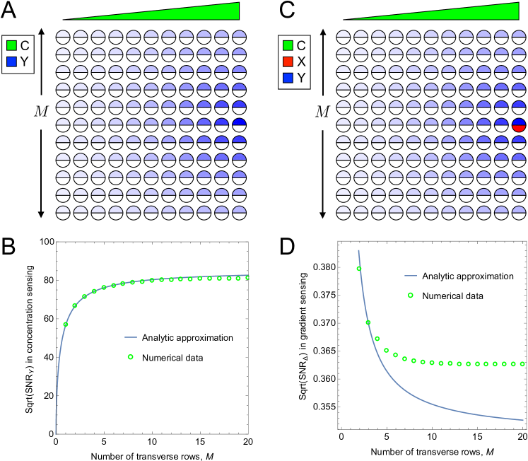
Figure 1: Spatial averaging transverse to a gradient improves concentration sensing, but worsens gradient sensing. (A) A 2-D array of cells is exposed to a concentration profile C that varies linearly in the horizontal direction (green wedge). In each cell, Y molecules are produced in proportion to the local C value. Y molecules are also exchanged between neighboring cells, providing the spatial averaging. Thus Y is the readout for the average concentration in the vicinity of a particular cell. Blue indicates the mean number of Y molecules $\bar{y}$ in each cell that have originated from the rightmost, middle cell. (B) The signal-to-noise ratio (SNR) for $y$ increases with the number $M$ of rows of cells added transverse to the gradient direction. (C) As in A, but with an additional internal species X. The molecules are also produced in proportion to the local C value, but they are not exchanged between cells. Red indicates the mean number of X molecules $\bar{x}$ in each cell that have originated from the rightmost, middle cell. The difference $\Delta=x-y$ provides the readout for the gradient (LEGI). (D) In contrast to B, the SNR for $\Delta$ decreases with the number of transverse rows $M$. In B and D, the numerical results are compared with the theoretical approximations (see Eqs. 15 and 16, respectively) and agree at small $M$ as expected. Parameters are similar to the experiments in [12]: $\bar{c}_{N}=1.25$ nM, $g=0.5$ nM/mm, $a=10$ $\mu$m, $n_{y}=4$, $N=50$ cells per row, and $G=10$.

In the LEGI paradigm, X excites a downstream species while Y inhibits it. If the cell is at the higher edge of the gradient, then the local concentration (X) is higher than the spatial average (Y), and the excitation exceeds the inhibition. While such comparison of the excitation and the inhibition can be done by many different molecular mechanisms [19], we consider here the limit of shallow gradients, where the comparison is equivalent to subtracting Y from X [12]. This difference, $\Delta_{n}=x_{n}-y_{n}$, is the readout of the model. If $\Delta_{n}$ is positive, the $n$th cell is further up the gradient than average; if $\Delta_{n}$ is negative, the $n$th cell is further down the gradient than average. In this work, we always focus on the readout $\Delta_{N}$ of the cell highest up the gradient, which we denote as the $N$th cell.

We assume that the cells do not average concentrations of the signal C and the messenger molecules X and Y over time (though generalizations with averaging are certainly possible [20]). Then the precision of gradient sensing is given by the square root of the instantaneous signal-to-noise ratio (SNR) for the readout, SNR${}_{\Delta}=(\bar{\Delta}_{N}/\delta\Delta_{N})^{2}$, where the mean and variance are given by [12]

$$\bar{\Delta}_{N} = \bar{x}_{N}-\bar{y}_{N},$$ (3)

$$\bar{x}_{N} = Ga^{3}\bar{c}_{N},$$ (4)

$$\bar{y}_{N} = Ga^{3}\sum_{n}K^{y}_{n}\bar{c}_{N-n},$$ (5)

and

$$(\delta\Delta_{N})^{2} = (\delta x_{N})^{2}+(\delta y_{N})^{2}-2{\rm cov}(x_{N},y_{N}),$$ (6)

$$(\delta x_{N})^{2} = \bar{x}_{N}+G^{2}a^{3}\bar{c}_{N},$$ (7)

$$(\delta y_{N})^{2} = \bar{y}_{N}+G^{2}a^{3}\sum_{n}(K^{y}_{n})^{2}\bar{c}_{N-n},$$ (8)

$${\rm cov}(x_{N},y_{N}) = G^{2}a^{3}K^{y}_{0}\bar{c}_{N},$$ (9)

respectively. Here $K^{y}_{n}\equiv(M^{y})^{-1}_{N,N-n}$ is the communication kernel, and $G\equiv\beta/\mu$ is the gain. The first terms in Eqs. 7 and 8 correspond to intrinsic noise, while the second terms correspond to extrinsic noise and assume that the diffusion of the signal is slow [12]. Computing the precision for a given configuration of cells only requires inverting the connectivity matrix $M^{y}$.

In a 1-D geometry, and in the limit of many cells ($N\gg 1$) and fast communication ($\gamma_{y}\gg\mu$), the kernel reduces to $K^{y}_{n}\approx e^{-n/n_{y}}/n_{y}$, where $n_{y}\equiv\sqrt{\gamma_{y}/\mu}$ sets the effective length scale of communication [12]. In this limit, the variance in the global species and the covariance reduce to [12]

$$(\delta y_{N})^{2} \approx \bar{y}_{N}+G^{2}a^{3}\frac{\bar{c}_{N-n_{y}/2}}{2n_{y}},$$ (10)

$${\rm cov}(x_{N},y_{N}) \approx G^{2}a^{3}\frac{\bar{c}_{N}}{n_{y}}.$$ (11)

In the recently introduced regional excitation–global inhibition (REGI) model [20], the local species X is also exchanged among cells, but at a lower rate $\gamma_{x}<\gamma_{y}$. Then Eq. 1 becomes analogous to Eq. 2, and Eqs. 4, 7, and 9 are replaced by

$$\bar{x}_{N} = Ga^{3}\sum_{n}K^{x}_{n}\bar{c}_{N-n},$$ (12)

$$(\delta x_{N})^{2} = \bar{x}_{N}+G^{2}a^{3}\sum_{n}(K^{x}_{n})^{2}\bar{c}_{N-n},$$ (13)

$${\rm cov}(x_{N},y_{N}) = G^{2}a^{3}\sum_{n}K^{x}_{n}K^{y}_{n}\bar{c}_{N-n},$$ (14)

respectively, where $K^{x}_{n}\equiv(M^{x})^{-1}_{N,N-n}$ is the communication kernel for the local species, and $M^{x}_{nn^{\prime}}\equiv(1+|{\cal N}_{n}|\gamma_{x}/\mu)\delta_{nn^{\prime}}-(\gamma_{x}/\mu)\delta_{n^{\prime}\in{\cal N}_{n}}$. Once more, computing the precision for a given configuration of cells in the REGI model only requires inverting the connectivity matrices $M^{x}$ and $M^{y}$. While diffusion of X decreases $\bar{x}_{N}$ at the $N$th cell, and hence decreases the difference $\bar{\Delta}_{N}$, it also averages X over a larger volume, hence decreasing its noise. As shown in Ref. [20], under a broad range of conditions, the decrease in the noise dominates, and the overall precision of the REGI model is higher than that of LEGI.

3 Results

3.1 Concentration sensing precision increases with transverse detector size

Before investigating gradient sensing, we focus on the simpler problem of concentration sensing. In the local excitation–global inhibition (LEGI) model, both X and Y provide readouts of the local concentration, while their difference $\Delta$ provides a readout of the gradient. The concentration readout provided by Y is spatially averaged, whereas the concentration readout provided by X is not. Even if the signal profile is graded, X and Y are concentration readouts if viewed independently (with different spatial averaging), not gradient readouts. For example, during Drosophila development, the morphogen profiles are graded, but individual nuclei in the embryo measure (and threshold) the local concentration, possibly with some spatial averaging [21, 23, 24, 25].

How does the precision of concentration sensing depend on transverse detector size? To answer this question, we focus on the spatially averaged concentration readout Y. We consider a linear signal profile with gradient $g$ and compute the SNR of Y in the $N$th cell, as we vary the number $M$ of rows of cells in a direction transverse to the gradient (Fig. 1A). We see in Fig. 1B (green circles) that the precision of concentration sensing increases with $M$. The reason is that adding rows of cells transverse to the gradient allows for Y molecules to be exchanged between rows (in addition to along each row). This does not change the mean $\bar{y}_{N}$ due to the translational symmetry in the transverse direction. However, it does reduce the variance, since the global species Y is now averaged over more cells. The net effect is an increase in the SNR beyond what is allowed by longitudinal averaging.

We can elucidate the effect of spatial averaging more quantitatively by appealing to the expression for the variance in Y in a single row of cells, in the limit of many cells and fast communication (Eq. 10). For a small number of added rows ($M<n_{y}$, where $n_{y}$ is the lengthscale of the spatial averaging), we make the approximation that the averaging is nearly uniform over all $M$ rows. In this case, the intrinsic component of the variance is unchanged (since the mean is unchanged), but the extrinsic component is reduced by $M$,

$$(\delta y_{N})^{2}\approx\bar{y}_{N}+G^{2}a^{3}\frac{\bar{c}_{N-n_{y}/2}}{2n_{y}M}.$$ (15)

The SNR calculated using this approximation is compared with the numerical result in Fig. 1B. We see that the approximation agrees with the numerical data, and that the agreement is best for small $M<n_{y}=4$, as expected.

3.2 Gradient sensing precision decreases with transverse detector size

We now turn our attention to gradient sensing. How does the precision of gradient sensing depend on transverse detector size? To answer this question for a linear signal profile, we compute the SNR of the gradient readout $\Delta_{N}$ as a function of the number $M$ of rows of cells in a direction transverse to the gradient (Fig. 1C). We see in Fig. 1D that the precision of gradient sensing decreases with $M$ (green circles). This is in contrast to the precision of concentration sensing, which increases with $M$ (Fig. 1B).

To understand why the precision of gradient sensing decreases with $M$, we once again consider the mean and the variance of the readout. The mean $\bar{\Delta}_{N}=\bar{x}_{N}-\bar{y}_{N}$ does not change with $M$ because neither $\bar{x}_{N}$ nor $\bar{y}_{N}$ change with $M$. However, the variance $(\delta\Delta_{N})^{2}=(\delta x_{N})^{2}+(\delta y_{N})^{2}-2{\rm cov}(x_{N},y_{N})$ changes with $M$ due to two effects. First, the variance in the global species $(\delta y_{N})^{2}$ decreases with $M$ due to spatial averaging, as discussed in the previous section. Second, the covariance ${\rm cov}(x_{N},y_{N})$ also decreases with $M$ because Y is exchanged with a larger number of cells, whereas X is not exchanged, so the two covary more weakly. The effects have opposite signs. To understand which effect dominates, we again appeal to the expressions for a single row of cells in the limit of many cells and fast communication (Eqs. 10 and 11). For small $M<n_{y}$, if we make the approximation that the averaging is nearly uniform over all $M$ rows, then both (i) the extrinsic component of the variance in Y and (ii) the covariance are reduced by $M$,

$$(\delta\Delta_{N})^{2} \approx (\delta x_{N})^{2}+\bar{y}_{N}+G^{2}a^{3}\frac{\bar{c}_{N-n_{y}/2}}{2n_{y}M}-2G^{2}a^{3}\frac{\bar{c}_{N}}{n_{y}M}$$ (16)

$$= (\delta x_{N})^{2}+\bar{y}_{N}-G^{2}a^{3}\frac{[4\bar{c}_{N}-\bar{c}_{N-n_{y}/2}]}{2n_{y}M}.$$

Because the $N$th cell is at the highest concentration, we have $\bar{c}_{N}>\bar{c}_{N-n_{y}/2}$, and we see that Eq. 16 is a decreasing function of $M$. Therefore, the decrease of the covariance dominates over the decrease of the variance in Y, for all parameter values. Because the mean $\bar{\Delta}_{N}$ does not change with $M$, we conclude that the precision of gradient sensing decreases with transverse detector size. The SNR calculated using this approximation is compared with the numerical result in Fig. 1D. We see that the approximation agrees with the numerical data for small $M<n_{y}=4$, as expected. The disagreement at large $M$ is more apparent here than in Fig. 1B because the precision of gradient sensing is low compared to the precision of concentration sensing, i. e. the gradient is shallow compared to the background concentration.

3.3 REGI mechanism recovers the benefit of transverse averaging

In the previous section we saw that the precision of gradient sensing using the LEGI model (local messenger X is not exchanged among the cells) decreases with the size of a detector in a direction transverse to the gradient, due to the fact that the covariance between the subtracted variables decreases with the transverse size. For the REGI model, exchange of the X molecules has an additional effect beyond increasing the sensing precision for 1-D line of cells [20]: it increases the covariance of X and Y, compared to the LEGI mechanism. Indeed, now both X and Y are amplified, downstream signals from some of the same external ligand molecules. Since the decrease of gradient sensing precision with transverse detector size is due to the loss of covariance (Fig. 1D), this raises the question of whether the REGI strategy can overcome this effect and allow gradient sensing precision to benefit from transverse averaging.

To answer this question, we once again consider a linear signal profile, and we compute the SNR of the gradient readout $\Delta_{N}$ under the REGI model (see Background), as a function of the number $M$ of rows of cells in a direction transverse to the gradient (Fig. 2A). We see in Fig. 2B that for a sufficiently large value of $n_{x}\equiv\sqrt{\gamma_{x}/\mu}$, which sets the lengthscale of spatial averaging for the local species, the precision of gradient sensing increases with $M$. This is in contrast to the case of LEGI, for which the precision decreases with $M$ (Fig. 1D and black curve in Fig. 2B). Therefore, the recovery of covariance between X and Y in the REGI mechanism avoids the loss of gradient sensing precision and restores the benefit of transverse averaging.

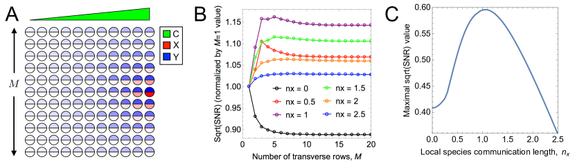
Figure 2: The regional excitation–global inhibition (REGI) strategy allows cells to exploit transverse spatial averaging for gradient sensing. (A) As in Fig. 1C, but for REGI. X molecules are exchanged between neighboring cells, at a lower rate than Y molecules. The difference $\Delta=x-y$ still provides the readout for the gradient. (B) In contrast to Fig. 1D, for sufficiently large communication length $n_{x}$ the SNR increases with the number of transverse rows $M$, before ultimately decreasing, which leads to an optimum as a function of $M$. (C) Since $n_{x}=0$ (LEGI) and $n_{x}=n_{y}$ (no sensing) are suboptimal, a global optimum emerges over both $M$ and $n_{x}$. Parameters are as in Fig. 1, with $n_{x}=1$ in A, which is near its optimal value according to C .

We also see in Fig. 2B that a maximal precision emerges in the REGI model as a function of $M$ at a particular number of rows $M^{*}$. This maximum is due to the fact that the exchange of $X$, which causes an increase in precision with $M$, and the exchange of $Y$, which causes a decrease in precision with $M$, occur on different length scales, $n_{x}<n_{y}$. Indeed, we see that as $n_{x}$ increases, the location of the maximum $M^{*}$ increases concomitantly. Additionally, we see in Fig. 2C that the maximal precision value first increases with $n_{x}$, then decreases with $n_{x}$, leading to an optimal value $n_{x}^{*}$. This is due to the previously understood tradeoff that is introduced when $n_{x}$ increases: on the one hand the variance of X is reduced, which increases precision; on the other hand, the means of X and Y are more similar, which decreases the precision [20]. Here this tradeoff is modified by the additional benefit of increasing $n_{x}$, namely that it increases the covariance of X and Y in the transverse direction, and thus further reduces the noise in gradient sensing.

3.4 Emergence of optimal detector shapes in two and three dimensions

The emergence of an optimal number of transverse rows of cells, seen in the previous section, raises the more general question of whether there is an optimal detector shape for spatially extended gradient sensing. This question has relevance for both 2-D and 3-D multicellular geometries involved in gradient sensing. Is the optimal detector shape more “hairlike”, to maximize its extent in the gradient direction, or more “globular”, to exploit potential benefits of extending along the transverse direction?

To address this question, we perform a controlled optimization for both 2-D and 3-D multicellular geometries. For a fixed number of cells $N=50$, we confine cells to an elliptical (2-D) or ellipsoidal (3-D) envelope, and compute the precision of gradient sensing as a function of the ellipse axis parameters (LEGI), as well as the ratio of averaging length scales $n_{x}/n_{y}$ (REGI), exhaustively exploring substantial ranges of both. In addition to the extra shape parameter, there is one more important difference between the 2-D and 3-D cases: in the 2-D case, we assume that every cell detects signal molecules, since we imagine that these molecules diffuse in the 3-D bulk, while the cells form a sensory sheet exposed to the bulk. In contrast, in the 3-D case, we assume that only the surface cells detect signal molecules, whereas cells that are blocked on all six sides by neighboring cells are “shielded” and thus do not detect signal molecules (although all cells still communicate via molecule exchange). The optimal detector shapes determined by such exhaustive search for the REGI model are shown in Fig. 3A, for 2-D (top) and 3-D (bottom).

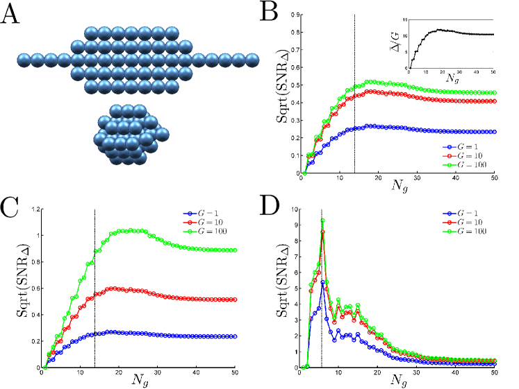
Figure 3: Optimal gradient sensing by 2-D and 3-D detectors. (A) Optimal elliptical (2-D, top) or ellipsoidal (3-D, bottom) configurations of $N=50$ cells for the REGI model. Gradient sensing precision is optimized at the rightmost cell, and the signal profile increases linearly to the right. We see that the optimal shapes are “globular”, not “hairlike”, especially in 3-D. (B) Precision vs. $N_{g}$ (the projected number of cells in the gradient direction) for the LEGI model in 2-D, for various gains $G$. Inset: mean readout $\bar{\Delta}$ normalized by $G$ (all three curves overlap and are colored black). (C) As in B, but for REGI. The additional REGI parameter $n_{x}$ is optimized over at each $N_{g}$ value, and the optimal precision is shown. At the observed optima in C, these values are $n_{x}^{*}/n_{y}=0.09$ ($G=1$), $0.30$ ($G=10$), and $0.53$ ($G=100$). (D) As in B but for 3-D. Internal cells are shielded and do not sense, but do communicate. Ellipsoid axes transverse to gradient are equal. Optimal $n_{x}^{*}=0$ for all $N_{g}$. Curve jaggedness arises due to numerical effects of fitting a cubic lattice of cells in a smooth ellipsoidal envelope. Black vertical dashed lines correspond to a perfect circle (B, C) or sphere (D). Parameters are as in Fig. 1.

To explain why these optimal shapes emerge, we present the precision of gradient sensing as a function of the control parameters. First we investigate the behavior of the LEGI model in 2-D (Fig. 3B). The control parameter is $N_{g}$, the (projected) number of cells in the gradient direction, which is set uniquely in 2-D by the ratio of the ellipse axis parameters. Small $N_{g}\to 1$ corresponds to a chain of cells transverse to the gradient, while large $N_{g}\to N$ corresponds to a chain of cells parallel to the gradient. The small “stair steps” in the curves are due to the numerical task of fitting the discrete multicellular square lattice within the continuous elliptical envelope. We see that the precision vanishes at $N_{g}=1$, as expected, since in our model a single cell cannot perform gradient detection. The precision is near maximal at $N_{g}=N$. This trend is analogous to that seen for LEGI in Fig. 1D, where here $N/N_{g}\sim M$ is the analog of the number of transverse rows. However, unlike in Fig. 1D, we see in Fig. 3B that there is a weak optimum at an intermediate value of $N_{g}$. This is due to a difference between the protocols of adding rows of cells (Fig. 1D) and reshaping a fixed number of cells (Fig. 3B). Adding rows does not change $\bar{\Delta}_{N}$. In contrast, as seen in the inset of Fig. 3B, reshaping changes $\bar{\Delta}_{N}$. The reason is that elliptical configurations (like Fig. 3A, top) are not translationally symmetric in the transverse direction. In particular, a large density of cells in the middle of the configuration is a sink for molecules of Y. This decreases the mean number of Y in the rightmost cell, $\bar{y}_{N}$, which weakly increases the signal $\bar{\Delta}_{N}=\bar{x}_{N}-\bar{y}_{N}$ at intermediate values of $N_{g}$ (Fig. 3B inset), and therefore increases the precision (Fig. 3B). Finally, we see that the precision increases with the gain $G$, as expected, and that the increase saturates with $G$, since then the variance of X and Y is dominated entirely by extrinsic, and not intrinsic, noise (see Background).

Next we investigate the behavior of REGI in 2-D (Fig. 3C). Once again the control parameter is $N_{g}$. Additionally, at every $N_{g}$ we optimize the local species’ averaging length scale $n_{x}$ (generally we find an optimal value between $\sim$$0.1n_{y}$ and $\sim$$0.5n_{y}$, see Fig. 3). We see in Fig. 3C that the trend of precision versus $N_{g}$ is similar to that of the LEGI model (Fig. 3C), but with two key differences. First, the precision is higher for REGI than for LEGI. This is due to regional averaging reducing the variance of the local species, as was known previously for the 1-D model [20]. Second, the optimum in the precision as a function of $N_{g}$ is more pronounced for REGI than for LEGI. This is because the region surrounding the optimum corresponds to near-circular ellipses, where considerable transverse averaging occurs. As shown in the previous section, transverse averaging increases precision in the REGI model. Overall, the optimal structure (Fig. 3A, top) is closer to a “globular” circle than to “hairlike” chain (compare locations of the optima to the dashed vertical line in Fig. 3C, which corresponds to a perfect circle). Therefore, we see that optimal gradient sensing by a 2-D structure benefits from an elliptical shape in which transverse averaging occurs.

Finally, we investigate the behavior of REGI in 3-D (Fig. 3D). Here there are two control parameters: the number of cells in the gradient direction $N_{g}$, and the asymmetry of the ellipsoid in the two directions transverse to the gradient. Generally we find that the optimal shape at a fixed $N_{g}$ displays symmetry in the two transverse directions, and therefore we impose this symmetry explicitly and focus on the control parameter $N_{g}$. As before, at every $N_{g}$ we optimize the local species’ averaging length scale $n_{x}$. Importantly, in the 3-D geometry, we find that the optimal value at every $N_{g}$ is $n_{x}^{*}=0$, corresponding to no averaging of the local species (an effective LEGI model). This is due to the shielding of internal cells: since internal cells do not detect signal molecules, averaging of the local species would dramatically reduce the mean local readout, making it far less than the actual local signal value at the edge cell. This would severely reduce the mean $\bar{\Delta}_{N}$, and thus the precision. The dependence of precision on $N_{g}$ is shown in Fig. 3D. The additional jaggedness is again due to the incommensurate nature of the cubic cell lattice with the smooth ellipsoidal envelope, here amplified due to the additional dimension. We see in Fig. 3D that there is again an optimum. In fact, it is much more pronounced than in 2-D: the overall value of the precision is ten-fold higher than in 2-D. This is again due to the shielding of internal cells: the global species Y is averaged among internal cells that do not produce it, which sharply decreases $\bar{y}_{N}$, and thereby increases $\bar{\Delta}_{N}$ and thus the precision. Overall, the optimal structure is very “globular” (Fig. 3A, bottom). Indeed, it is almost a sphere (compare the optima to the dashed vertical line in Fig. 3D). We conclude that, due to the combined effects of spatial averaging and shielding, the optimal 3-D detector of linear gradients extends significantly in all three spatial dimensions.

4 Discussion

We have investigated theoretically and computationally the ways in which the precision of spatially extended, multi-component gradient sensing is affected by detector geometry. Using a minimal model of adaptive gradient sensing (LEGI), we have found that, unlike for concentration sensing, the precision of gradient sensing decreases with the size of the detector in a direction transverse to the gradient. This is due to the competing effects of noise reduction and a reduction of the covariance between concentrations subtracted to estimate the gradient. We have demonstrated that a simple modification of LEGI (REGI) restores the covariance and recovers the benefit of transverse averaging for gradient sensing. The result is that the optimal detectors in 2-D and 3-D are more globular than hairlike.

Our study elucidates the important roles of spatial averaging in gradient sensing, which are several-fold. First, there is spatial averaging along the gradient. In both LEGI and REGI, the global species Y is averaged along the gradient. For a linear signal profile, this averaging both increases the signal $\bar{\Delta}^{2}$, and decreases the noise $(\delta{\Delta})^{2}$. Therefore, it is optimal for Y to be averaged along the gradient to as large an extent as possible. Second, in the REGI model, the local species X is also averaged along the gradient. This decreases the signal but also decreases the noise [20]. Therefore, there is often an optimal ratio $n_{x}/n_{y}$ of the spatial extents of the averaging. Third, there is spatial averaging transverse to the gradient. In the LEGI model, only Y is averaged transverse to the gradient. In a translationally symmetric geometry, this does not change the signal, but it changes the noise by both decreasing the variance of Y and decreasing the covariance between X and Y. These have opposite effects on the precision. For LEGI, the latter dominates, decreasing the precision. Therefore, transverse averaging is detrimental for gradient sensing. However, in the REGI model, X is also averaged transverse to the gradient. Once again, in a translationally symmetric geometry, this does not change the signal with respect to REGI in 1-D, but it decreases the noise, both by further reducing the variance in X and by restoring a larger covariance between X and Y. Therefore, transverse averaging is beneficial for REGI-type gradient sensing. These roles of spatial averaging are modified in geometries without translational symmetry as we discussed above. However, the net result remains the same: the optimal 2-D and 3-D REGI-type gradient detectors are globular, benefitting from extensive spatial averaging in the transverse directions.

Our study also reveals the effects of shielding of signal from the inner cells in a 3-D geometry. Shielding amplifies the effect of spatial averaging, since the measurements performed by edge cells, which detect signal, are averaged with those of their interior neighbors, which do not detect signal. This amplification increases the signal in a particular edge cell, but makes the system less adaptive, since every edge cell has an above-average readout. With shielding, a more appropriate measure of the sensory outcome might therefore be the difference in readouts between cells up and down the gradient, e. g. $\bar{\Delta}_{N}-\bar{\Delta}_{1}$. This measure is likely to depend nontrivially on internal and geometric parameters such as $n_{x}$ and $M$, and will likely result in a nontrivial optimal local averaging length scale, $n_{x}^{*}\neq 0$. Another possibility is that gain $G$ should be different in Eqs. 4 and 5, compensating for the two messenger molecules averaging over different numbers of neighbors that do not detect the ligand. We leave both of these interesting explorations for future investigations.

In this work, we have emphasized the distinction between (i) concentration sensing within a graded concentration profile and (ii) gradient sensing. For example, in Drosophila development, individual nuclei in the embryo measure (and are thought to threshold) the local concentration, even though the morphogen gradient is graded [21, 23, 24, 25]. This is an example of concentration sensing. In contrast, gradient sensing, as explored here, is the task of obtaining an internal readout of the difference in local signal concentrations at two or more different points in space. In other words, unlike concentration sensing, gradient sensing determines the direction in which the concentration changes, and it allows subsequent directional polarization of the sensor. This definition of gradient sensing, by construction, is adaptive: the readout does not depend on the background concentration. Systems that respond adaptively and directionally to chemical gradients, such as amoeba [27] and epithelial cell groups [12], are preforming gradient sensing. Because concentration sensing and gradient sensing are distinct, it may not be so surprising that transverse averaging has very different effects on them: the precision of concentration sensing increases with the transverse size, whereas the precision of LEGI gradient sensing decreases with the transverse size (Fig. 1).

How do our results compare to experimental systems? A well-studied example of a natural gradient-sensing system is the growth factor-directed extension of mammary epithelial ducts [22, 10]. Gradient sensing in this system has been shown to be multicellular and adaptive [12]. In vivo, the extension is led by an “end bud” of cells at the duct tip. These tips can form either long hairlike structures or coalesce into nearly spherical globules, as was observed in organotypic studies with different chemical and genetic perturbations [12]. Long hairs could act as “feelers” for the duct, sampling a long swath of the environment in the gradient direction. However, our analysis predicts that such hairlike morphologies are suboptimal, and the globular bud shape, as in Fig. 3A, would produce a better precision. In agreement with the prediction, the end buds in wildtype mice are nearly spherical, and the globule is often wider than the duct itself [10]. Similarly, neither chemotaxing amoeba [27] and neutrophils [2], nor growing neurons [1] form very thin hairlike protrusions to facilitate sensing. Instead they keep the aspect ratio of the gradient sensing part of the protrusions closer to one, again supporting our findings. Further, in Drosophila border cell migration, another example of directional collective cell behavior, groups of cells travel as a sphere in a confined space, where it would have been easier to travel as a chain [5]. All of these examples provide indirect evidence that transverse averaging is used in multiple biological contexts. While direct tests of effects of transverse averaging have not been done, they are certainly possible. Indeed, as mentioned above, different perturbations to organotypic epithelial cultures result in them assuming different geometric shapes [12]. Thus it should be possible to measure the accuracy of sensing (and the subsequent organoid polarization) as a function of the shape. Such experiments would allow direct testing of our main prediction that transverse averaging leads to more accurate directional sensing outcomes, especially in REGI-type models.

References

References

- [1] Rosoff W J, Urbach J S, Esrick M A, Mcallister R G, Richards L J and Goodhill G J 2004 Nat Neurosci 7 678–82
- [2] Onsum M D, Wong K, Herzmark P, Bourne H R and Arkin A P 2006 Phys Biol 3 190–199
- [3] Song L, Nadkarni S M, Bödeker H U, Beta C, Bae A, Franck C, Rappel W J, Loomis W F and Bodenschatz E 2006 Eur J Cell Biol 85 981–9
- [4] Sternlicht M D, Kouros-Mehr H, Lu P and Werb Z 2006 Differentiation 74 365–381
- [5] Bianco A, Poukkula M, Cliffe A, Mathieu J, Luque C, Fulga T and Rørth P 2007 Nature 448 362–365
- [6] Friedl P and Gilmour D 2009 Nat Rev Mol Cell Biol 10 445–457
- [7] Mani M, Goyal S, Irvine K D and Shraiman B I 2013 Proceedings of the National Academy of Sciences 110 20420–20425
- [8] Donà E, Barry J D, Valentin G, Quirin C, Khmelinskii A, Kunze A, Durdu S, Newton L R, Fernandez-Minan A, Huber W, Knop M and Gilmour D 2013 Nature 503 285–289
- [9] Pocha S M and Montell D J 2014 Annual review of genetics 48 295–318
- [10] Huebner R J and Ewald A J 2014 Seminars in cell & developmental biology 31 124–131
- [11] Malet-Engra G, Yu W, Oldani A, Rey-Barroso J, Gov N S, Scita G and Dupré L 2015 Curr Biol 25 242–250
- [12] Ellison D, Mugler A, Brennan M, Lee S H, Huebner R, Shamir E, Woo L A, Kim J, Amar P, Nemenman I et al. 2015 Proceedings of the National Academy of Sciences, USA Accepted (arXiv preprint arXiv:1508.04692)
- [13] Berg H C and Purcell E M 1977 Biophys J 20 193–219
- [14] Goodhill G J and Urbach J S 1999 J Neurobiol 41 230–41
- [15] Levchenko A and Iglesias P A 2002 Biophysical Journal 82 50–63
- [16] Endres R G and Wingreen N S 2008 Proc Natl Acad Sci USA 105 15749–54
- [17] Endres R G and Wingreen N S 2009 Progr Biophys Mol Biol 100 33–9
- [18] Hu B, Chen W, Rappel W J and Levine H 2010 Physical Review Letters 105 48104
- [19] Jilkine A and Edelstein-Keshet L 2011 PLoS Comp Biol 7 e1001121
- [20] Mugler A, Levchenko A and Nemenman I 2015 Proceedings of the National Academy of Sciences, USA Accepted (arXiv preprint arXiv:1505.04346)
- [21] Gregor T, Tank D W, Wieschaus E F and Bialek W 2007 Cell 130 153–164
- [22] Ewald A J, Brenot A, Duong M, Chan B S and Werb Z 2008 Developmental cell 14 570–581
- [23] Erdmann T, Howard M and Ten Wolde P R 2009 Physical review letters 103 258101
- [24] Lander A D 2011 Cell 144 955–969
- [25] Sokolowski T R and Tkacik G 2015 Phys Rev E 91 062710
- [26] Camley B A, Zimmermann J, Levine H and Rappel W J 2015 arXiv preprint arXiv:1506.06698
- [27] Swaney K, Huang C and Devreotes P 2010 Annu Rev Biophys 39 265––289