Dynamical Quantum Phase Transitions in presence of a spin bath

Abstract

We derive an effective time independent Hamiltonian for the transverse Ising model coupled to a spin bath, in the presence of a high frequency AC magnetic field. The spin blocking mechanism that removes the quantum phase transition can be suppressed by the AC field, allowing tunability of the quantum critical point. We calculate the phase diagram, including the nuclear spins, and apply the results to Quantum Ising systems with long-range dipolar interactions; the example of $LiHoF_{4}$ is discussed in detail.

I Introduction

“Quantum phase transitions” (QPT) take place between bulk equilibrium phases in the zero-temperature ($T\rightarrow 0$) limit. Hertz hertz showed that finite-$T$ thermodynamic and transport properties near the zero-$T$ quantum critical point (QCP) should be determined solely by the nature of the QCP itself. Classic examples are the Quantum Ising system, and the paramagnetic/ferromagnetic (PM/FM) transition in strongly-correlated conductors. However in real experimental systems things are not so simple: in zero-$T$ PM/FM transitions, disorder and 1st-order phase transitions often obscure the physics, and in solid-state Quantum Ising systems “environmental” spin bath modes spinB can suppress the QCP entirely aeppli05 ; RonnowPRB . This is unfortunate, given the importance of Quantum Ising phenomenology in so many areas of physics. There currently exists no good theory of QPT in Ising systems in the presence of a spin bath; however, the external control of the spin bath decoherence for qubits has been studied from the perspective of Nuclear Magnetic Resonance, where sequences of pulses are used to manipulate the coupling of qubits to the environmental modesDynamDeco ; Spin-bath-Dot ; Decoupling-Spinbath ; Decoupling-Spinbath2 ; Decoupling-NV .

In this work we address this problem by: (i) Enlarging the QPT scenario for Quantum Ising systems, by generalizing the theory to the case of a strong high-frequency AC field, and (ii) showing how in principle this allows the manipulation of the effective Ising Hamiltonian, enabling one to suppress the spin bath effects. The AC field creates a new effectively time-independent Hamiltonian for the system, inducing new interactions and suppressing others, thereby opening up a new class of QPTs for investigation. By varying the frequency, and intensity of the field, one also obtains a very rich zero-$T$ phase diagram, with various new kinds of QCP.

II Low energy Hamiltonian

Well-known solid-state examples of experimental Quantum Ising systems with long-range dipolar inter-spin interactions include the $LiHo_{x}Y_{1-x}F_{4}$ rare earth system (aeppli05 ; RonnowPRB and schechter05 -kycia-dyn ), and the transition metal-based $Fe_{8}$ molecular spin system takahashi . Recent experiments on 1-dimensional ion trap Quantum Ising chains (where spin bath effects may be entirely absent) have also successfully varied the range of the interactions ionChain1 ; ionChain2 . These systems are all described at low energies by Hamiltonians with spins $\vec{\tau}_{i}$ truncated to the lowest Ising doublet (i.e., to its doubly degenerate ground state), separated from the next level by a gap $\Lambda_{o}\gg|V_{i,j}|,|A|$, where $V_{i,j}$ and $A$ are the strengths of the inter-spin and hyperfine couplings. Then, their low energy behavior reduces to the study of the next Ising type Hamiltonian:

$$H\left(t\right)=-\sum_{i=1}^{N}\left[\Delta_{o}+\Gamma\left(t\right)\right]\tau_{i}^{x}-\sum_{i<j}V_{i,j}\tau_{i}^{z}\tau_{j}^{z}+H_{\textrm{HF}}$$ (1)

The total effective field here is the sum of a constant $\Delta_{o}$ and a time-dependent $\Gamma\left(t\right)$. Typically these are not real magnetic fields, but effective fields acting in the Hilbert space of the Ising doublet. Then, it is useful to briefly describe the truncation procedure: The low-energy effective Hamiltonian is truncated from a microscopic spin Hamiltonian of the form:

$$H_{M}\left(t\right) = -\sum_{i}H_{o}\left(\boldsymbol{S}_{i}\right)+\left[\mathcal{B}_{x}+H_{x}\left(t\right)\right]S_{i}^{x}$$

$$-\frac{1}{2}\sum_{i,j\neq i}U_{i,j}S_{i}^{z}S_{j}^{z}+H_{\textrm{HF}}^{M}$$

where $H_{o}\left(\boldsymbol{S}_{i}\right)$, the local ”high-energy” ionic spin Hamiltonian, acts on spins $\left\{{\bf S}_{j}\right\}$. The Hilbert space for each magnetic ion now has dimension $2S+1$. The high-energy hyperfine coupling takes the form:

$$H_{\textrm{HF}}^{M} = \sum_{\mu,\nu}\sum_{j,k}\Lambda_{j,k}^{\mu\nu}S_{j}^{\mu}I_{k}^{\nu}$$ (3)

where we use a slightly unconventional notation in which $\Lambda_{jk}^{\mu\nu}$ denotes the ”bare” hyperfine coupling between the full spin ${\bf S}_{j}$ and the nuclear spin ${\bf I}_{k}$, and drop the nuclear quadrupolar couplings, which are negligible for the quantum Ising systems examined so far. While the low-energy form (Eq.1) is generic to all of the Quantum Ising systems so far investigated, the high-energy form (Eq.II) varies widely from one physical system to another, depending on the magnitude of the ${\bf S}_{j}$, the lattice symmetry, the strength of the spin-orbit, crystal field, hyperfine fields, and so on. Thus the details of the truncation, of the dependence of the low-energy fields $\Delta_{o}$ and $\Gamma\left(t\right)$ on the external fields, and of the magnitude and anisotropy of the low-energy $A_{j,k}^{\mu\nu}$ and $V_{i,j}$, depend very much on which system we are looking at. We will discuss here the 3 cases:

$LiHo_{x}Y_{1-x}F_{4}$:

In this case, the high-energy Hamiltonian involves ionic spins with $S=8$ and a local spin Hamiltonian

$$H_{o}\left({\bf S}\right) = \sum_{k=4,6}R_{k}^{4}\left(C\right)\hat{O}_{k}^{4}\left(C\right)+R_{6}^{4}\left(S\right)\hat{O}_{6}^{4}\left(S\right)$$

$$+\sum_{k=2,4,6}R_{k}^{0}\hat{O}_{k}^{0}$$

written in terms of the standard Stevens operators $\hat{O}_{k}^{q}$ (see, eg., Jensen and MacKintosh Jensen ); the best values of the parameters $R_{k}^{q}$ are given by Ronnow et al aeppli05 ; RonnowPRB . This ”high-energy” form is valid up to energy scales $\sim 10^{3}$K. The truncation of the high-energy Hamiltonian of Eqs.II,II down to the low-energy form in Eq.1 has been thoroughly discussed in the literature aeppli05 ; RonnowPRB ; Chack2004 ; schechter05 . The low-energy form can be used for energies smaller than the gap of $\sim 11.3$K which exists between the low-energy spin doublet and a 3rd intermediate state, through which virtual transitions allow a coupling between the 2 lowest Ising states $|\Uparrow\rangle$ and $|\Downarrow\rangle$ on each site. The transition matrix element $\Delta_{o}\left(\mathcal{B}_{x}\right)$ between these states is a highly non-linear function of $\mathcal{B}_{x}$, obtainable by exact diagonalizationschechter05 . The hyperfine interactions are large: experiment shows that $\Lambda_{j,k}^{\mu\nu}\sim 0.039$K for the bare on-site $Ho$ hyperfine coupling, for which $I=7/2$, with considerably smaller values for the hyperfine couplings to the four $F$ nuclear spins. This then gives a splitting between adjacent hyperfine levels of $\sim 0.22$K, and a total spread of energy over the eight hyperfine levels of $\sim 1.5$K. Thus the hyperfine energy scale competes very well with the dipolar coupling $U_{i,j}$ between nearest neighbor $Ho$ ions, even for the pure $LiHo$ system, where the energy difference between $|\Uparrow\Uparrow\rangle$ and $|\Uparrow\Downarrow\rangle$ configurations coming from the dipolar interactions is also $\sim 1.5$K. For $Y$-doped $LiHo_{x}Y_{1-x}F_{4}$, this nearest neighbor dipole coupling is reduced by a factor $\sim O(x)$, and the hyperfine coupling then dominates.

The $Fe_{8}$ molecular spin system:

In this case the high-energy Hamiltonian has spin $S=10$ (coming from a core of eight $Fe$ ions), and a local spin Hamiltonian which is well approximated by

$$H_{o}\left({\bf S}\right)=-D_{o}S_{x}^{2}+E_{o}S_{y}^{2}-K_{4}\left(S_{+}^{4}+S_{-}^{4}\right)$$ (5)

where the values of $D_{o}$, $E_{o}$, and $K_{4}$ (all positive) were measured some time ago barra . This form can be used up to energy scales $\sim 50$K. Each $Fe_{8}$ molecule has up to 213 different nuclear spins, depending on which of the various $Fe,Br,N,O$, and $H$ isotopes in the molecule are being used; each of the hyperfine couplings for this system has been calculated, but they are typically very small (the proton couplings range from $\sim 3$mK down to well below $1$mK, except for the odd outlier, with similar values for the other non-metallic nuclear species; the coupling to isotopically substituted ${}^{57}Fe$ nuclei is $\sim 4$mK). Thus the inter-molecular dipolar coupling, of a similar magnitude to that for $LiHo$, is much larger. The truncation to the low-energy doublet form can again be done numerically MST06 , and is valid for energies smaller than the gap of $\sim 5$K to the next highest states. Again the dependence of $\Delta_{o}$ and $\Gamma\left(t\right)$ on a transverse field $\boldsymbol{\mathcal{B}}$ is very non-linear, and also varies enormously with the angle of the field in the easy $\hat{x}\hat{y}$-plane - for $\boldsymbol{\mathcal{B}}$ oriented along the easy $\hat{x}$-axis one sees very strong oscillations of $\Delta_{o}$ as a function of $\mathcal{B}_{x}$.

Ionic spin chains:

In this case one can, to a good approximation, begin by ignoring the coupling to a spin bath. The Hamiltonian in experiments ionChain1 ; ionChain2 ; ionChain3 can be more general than the standard Quantum Ising system, and the low energy form is:

$${\cal H}_{eff} = \Delta_{o}\sum_{j}\tau_{j}^{x}+\sum_{i\neq j}J_{i,j}^{zz}\tau_{i}^{z}\tau_{j}^{z}+{\cal H}_{J}^{\perp}$$ (6)

where the extra term is just an $XY$ form ${\cal H}_{J}^{\perp}=\sum_{i\neq j}J_{i,j}^{\perp}\left(\tau_{i}^{+}\tau_{j}^{-}+\tau_{i}^{-}\tau_{j}^{+}\right)$. The parameters $\Delta_{o}$ and $J_{i,j}^{\alpha\alpha}$ are again effective parameters, related to the original applied fields in ways described in detail in refs.ionChain1 ; ionChain2 ; ionChain3 . In different experiments with different ions one can vary these parameters over a rather wide range; typical values are $10^{-9}~{}K<J_{o}<10^{-7}~{}K$, and $10^{-2}<\Delta_{o}/J_{o}<5$, where $J_{o}$ is a typical nearest neighbor value for either $J_{i,j}^{zz}$ or $J_{i,j}^{\perp}$. The interactions typically take a power law form as a function of the distance $r_{ij}=a_{o}|i-j|$, where $a_{o}$ is the lattice spacing (typical $2-3\ \mu m$), ie., $|J_{i,j}^{\alpha\alpha}|\sim J_{o}|i-j|^{-p}$, where in principle one can vary $p$ between $1<p<3$. Provided $\Delta_{o}$ is not too large, the coupling to phonons can be adequately suppressed. The effective Hamiltonian found in this work applies when we ignore the ”easy-plane” or XY-coupling terms in (6), as the phase diagram with these terms added becomes very rich and requires a separate study.

III Magnus expansion

In what follows we will work exclusively with the low-energy effective Hamiltonian given in (1) above, because our topic is the behavior of a Quantum Ising system in a high-frequency AC field. Thus we will leave the behavior of the parameters $\Delta_{o}$, $\Gamma\left(t\right)$, $A_{jk}^{\mu\nu}$, and $V_{ij}$, as functions of the real applied fields, in the form of undetermined variables in this effective Hamiltonian, to be determined in practice by a combination of numerical calculation and experiment on whichever system one is dealing with.

The next step to find a time independent Hamiltonian is to approximate the full time evolution by a stroboscopic one, in terms of an effective Hamltonian. For that to be possible, we assume that the frequency $\omega$ of the time dependent field $\Gamma\left(t\right)$ falls in the range $\Lambda_{o}>\omega\gg|V_{i,j}|,|A|$. This allows us to describe the effects of the AC field on the quantum Ising system by a standard Magnus expansion Bastidas ; Modulated-Ising ; TI-QPT ; Blanes-Magnus ; Magnus-Floquet-Micromotion ; Floquet-Magnus-Mananga ; Goldman , in inverse powers of $\omega$. The Magnus expansion is a very powerful method to extract the stroboscopic time evolution of a time dependent system, when the frequency of the driving field is large. By means of a transformation to the interaction picture, ie., $H\left(t\right)\rightarrow\tilde{H}\left(t\right)=U_{1}H\left(t\right)U_{1}^{\dagger}-iU_{1}\dot{U}_{1}^{\dagger}$, where $U_{1}=e^{i\int dt\sum_{j}\mathbf{\Gamma}\left(t\right)\boldsymbol{\tau}_{j}^{x}}$, one can also capture the renormalization of parameters produced by non-perturbative effects of the field. The Magnus expansion then approximates the time dependent Hamiltonian by a time averaged one given by:

$$\mathcal{H} = \tilde{H}_{0}+\frac{1}{\omega}\sum_{n=1}^{\infty}\frac{1}{n}\left[\tilde{H}_{n},\tilde{H}_{-n}\right]$$ (7)

where $\tilde{H}_{n}$ is the $n$-th Fourier component of $\tilde{H}\left(t\right)$, and terms $\sim O\left(\left|A\right|/\omega^{m},\left|V_{i,j}\right|/\omega^{m}\right)$ ($m\geq 2$) are assumed negligible at high frequency.

In discussing a Magnus expansion, it is important to specify the ”initialization protocol”, ie., the way in which the AC applied field is ramped up at the beginning. One option often used is to use an ”adiabatic launching protocol” Goldman , which consists in reaching the final non-equilibrium steady state by keeping the system in the same quasienergy state. Heating can be a problem here, specially due to the spin-phonon couplings in the system, and the fact that interacting Floquet systems tend to evolve towards an infinite temperature, featureless stateInfinite-temperature . Nevertheless the spin-phonon couplings are typically rather weak for the Quantum Ising systems being currently studied; this means that it will take the phonon bath some time to react to the rapid oscillations of the electronic spins. Thus the use of pulsed fields is more appropriate, with widely spaced pulses, as the system then has time for energy relaxation between pulses. It would also be helpful to have a phonon bath for which the density of states for undesired Floquet transitions, which could drive the system out of the steady state, is small; this would stabilize the Floquet phase described in this work Population-Floquet . Finally, in order to avoid the tendency towards an infinite temperature state, one could try to control the non-adiabatic corrections during the adiabatic launching (as if it is ramped too slowly, the system will reach the infinite temperature state), or combine it with a many-body localized phase, which would prevent the system from thermalizingFloquet-MBL .

IV Dynamical quantum phase transition

As a warm up we first consider a ’pure’ Quantum Ising QPT, with no spin bath. We apply a linear AC field $\mathbf{\Gamma}\left(t\right)=\Gamma_{x}\cos\left(\omega t\right)$, and find that $\left[\tilde{H}_{n},\tilde{H}_{-n}\right]=0$ for all $n$, leaving only the zeroth Fourier component $\tilde{H}_{0}$ in Eq. (7) (see Appendix for details), and thus a time-independent effective Hamiltonian:

$$\mathcal{H}^{o} = -\sum_{i}\Delta_{o}\tau_{i}^{x}-\sum_{i,j>i}\left[\tilde{V}_{i,j}^{zz}\tau_{i}^{z}\tau_{j}^{z}+\tilde{V}_{i,j}^{yy}\tau_{i}^{y}\tau_{j}^{y}\right]$$ (8)

where $\tilde{V}_{i,j}^{zz}\left(\alpha\right)=V_{i,j}\left[1+\mathcal{J}_{0}\left(2\alpha\right)\right]/2$, $\tilde{V}_{i,j}^{yy}\left(\alpha\right)=V_{i,j}\left[1-\mathcal{J}_{0}\left(2\alpha\right)\right]/2$, the dimensionless parameter $\alpha=\Gamma_{x}/\omega$ and $\mathcal{J}_{m}\left(\alpha\right)$ is an $m$-th order Bessel function; the superscript in $\mathcal{H}^{o}$ indicates zero hyperfine couplings. Thus the periodic driving modifies the direction and strength of the inter-spin coupling tensor, and transforms the Ising model into an XY (strictly a YZ) model with anisotropy controlled by $\alpha$ (as previously shown by Bastidas in 1D). The anisotropic XY model has Ising phase transitions when the transverse magnetic field $\Delta_{0}=\pm\tilde{V}_{i,j}^{\mu\mu}$, as well as anisotropic transitions for $\tilde{V}_{ij}^{yy}=\tilde{V}_{ij}^{zz}$, where the magnetization changes its orientation between $M_{y}^{o}$ and $M_{z}^{o}$ (the super-index indicate the absence of a spin bath in this section). Note Eq.8 is valid in arbitrary dimension, but the dimensionality plays an important role when calculating the different statistical averages, as it is discussed next.

To characterize the QPT we must determine the magnetization (ie., the order parameter). For that, we calculate the double-time Green’s functionZubarev $G_{n,m}^{\alpha,\beta}\left(t,t^{\prime}\right)=-i\theta\left(t-t^{\prime}\right)\langle\left\{S_{n}^{\alpha}\left(t\right),S_{m}^{\beta}\left(t^{\prime}\right)\right\}\rangle$, using a $1/Z$ expansion to lowest order ($Z$ is the coordination number), which coincides with the Random Phase ApproximationRonnowPRB (RPA). Under this assumptions the Heisenberg equation of motion for the Green’s function simplifies to:

$$\omega G_{n,m}^{\alpha,\beta} = \frac{\langle\left\{S_{n}^{\alpha},S_{m}^{\beta}\right\}\rangle}{2\pi}+i\sum_{\mu}\epsilon_{\mu\alpha\delta}B_{\mu}G_{n,m}^{\delta,\beta}$$

$$+i\sum_{\mu}\epsilon_{\mu\alpha\delta}\left(\sum_{j\neq n}V_{n,j}^{\mu\mu}\langle S_{j}^{\mu}\rangle-\sum_{r}A_{r,n}^{\mu\mu}\langle I_{r}^{\mu}\rangle\right)G_{n,m}^{\delta,\beta}$$

and can be generally solved. Note that at this point we are considering a general magnetic field $B_{\mu}$ and interaction $V_{n,j}^{\mu\mu}$, as it does not complicate things. The last step is to relate the Green’s function with the magnetization using:

$$\langle S_{m}^{\beta}S_{n}^{\alpha}\rangle=i\int\frac{G_{n,m}^{\alpha,\beta}\left(\omega+i\epsilon\right)-G_{n,m}^{\alpha,\beta}\left(\omega-i\epsilon\right)}{e^{\beta\omega}+1}d\omega$$ (10)

and derive the “self consistency equation” (SCE) for the magnetization, which in absence of the spin bath, simply is:

$$M_{\mu}^{o} = \frac{B_{\mu}+M_{\mu}^{o}\tilde{V}_{0}^{\mu\mu}}{2\tilde{\omega}_{S}}\tanh\left(\frac{\beta\tilde{\omega}_{S}}{2}\right)$$ (11)

where $M_{\mu}^{o}$ ($\mu=x,y,z$) is the magnetization along the $\mu$-axis, $\tilde{\omega}_{S}=\sqrt{\sum_{\mu}\left(B_{\mu}+M_{\mu}^{o}\tilde{V}_{0}^{\mu\mu}\right)^{2}}$, the effective field is $B_{\mu}=\left(\Delta_{o},0,0\right)$, and $\tilde{V}_{0}^{\mu\mu}$ is the $\mathbf{q}=0$ Fourier component of the effective spin-spin interaction along the $\mu$-axis. The detailed derivation is delegated to the Appendix, as it closely follows the one of ref.Fermion-GF , with the addition of the spin bath.

Note that the formalism applied here is valid for arbitrary large spins (which is important to describe the $7/2$ spin bath in the next section). Also the $1/Z$ scaling implies that the results are expected to be more accurate in higher dimensional systems (where the coordination number is large), such as the 3D Ising model. Therefore our results for the magnetization will better describe the experiments on $LiHo_{x}Y_{1-x}F_{4}$, than the ones on ionic spin chains, where one would expect large quantum fluctuations which would modify the magnetization. The system’s dimension is encoded in the coordination number $Z$, or equivalently in the zeroth Fourier component of the interaction potential $V_{0}$. For the simplest case of nearest neighbor interaction, one finds that they are related by $V_{0}=ZV$, however in more general situations, as for the case of long-range dipolar interactions, this relationship fails and it is more convenient to just estimate $V_{0}$ by other means, keeping in mind that the system’s dimension is somehow encoded in this value. The inverse temperature $\beta$ in Eq.11 corresponds to the phonon bath temperature that in general, would couple to the spin system. Although its definition is not generally possible in the presence of a driving field, we will discuss in the last section how, under some circumstances, one can still make use of it.

Eq.11 allows to easily compare the AC driven and the undriven case. For the undriven ($\Gamma_{x}=0$) pure 3D Ising model we find the next ground state magnetization:

• For $\Delta_{o}<V_{0}^{zz}/2$:

  $$M_{x}^{0}=\frac{\Delta_{o}}{V_{0}^{zz}},\quad M_{y}^{0}=0,\quad M_{z}^{0}=\pm\frac{\sqrt{\left(V_{0}^{zz}\right)^{2}-4\Delta_{o}^{2}}}{2V_{0}^{zz}}.$$ (12)

• For $\Delta_{o}>V_{0}^{zz}/2$:

  $$M_{x}^{0}=\frac{1}{2},\quad M_{y,z}^{0}=0.$$ (13)

The critical field is given by $B_{c}=V_{0}^{zz}/2$, and the finite-$T$ solution gives a zero field Curie temperature $T_{c}=V_{0}^{zz}/4$. For the case of long-range dipolar interactions, present in $LiHo_{x}Y_{1-x}F_{4}$, one can directly estimate the zeroth Fourier component $V_{0}^{zz}$ by numerical meansRonnowPRB , or as we have done in our case, extract its value from experimental measurementsChack2004 . The phase diagram is shown in Fig.1, where the dashed black line separates a spin ordered FM phase for $\Delta_{o}<B_{c}$ and a paramagnetic one otherwise.

In the presence of the AC field the system is described by the anisotropic XY model (Eq.8). The anisotropy factor $\tilde{V}_{j,l}^{zz}-\tilde{V}_{j,l}^{yy}=\mathcal{J}_{0}\left(2\alpha\right)V_{j,l}$ becomes a function of $\alpha$ and the Ising model is recovered when $\mathcal{J}_{0}\left(2\alpha\right)=0$. This means that anisotropic quantum phase transitions happen every time $\mathcal{J}_{0}\left(2\alpha\right)=0$, and the magnetization changes its direction between $M_{z}^{o}$ and $M_{y}^{o}$ for temperatures below a critical $T_{c}$. Ising transitions could also be induced when $\alpha$ is tuned, as the critical field $B_{c}$ oscillates between a maximum and a minimum value (red solid line in Fig.2). Therefore, if the DC field is within this window, one would also observe PM/FM transitions.

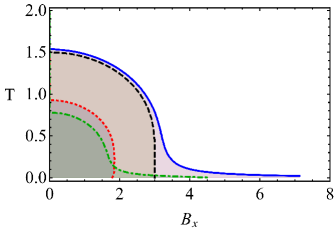
Figure 1: Phase diagram of the AC driven transverse Ising model vs transverse field $B_{x}$ and temperature. The dashed black line corresponds to the undriven system in absence of hyperfine coupling. The blue line corresponds to the undriven system coupled to the $I=7/2$ spin bath. The red line corresponds to the AC driven system coupled to the spin bath for $\Gamma_{x}/\omega\sim 2.4$ (i.e., $\mathcal{J}_{0}\left(\alpha\right)=0$). The green line corresponds to the case $2\Gamma_{x}/\omega\sim 2.4$, where the spin-spin interaction is symmetrical and resembles the Ising system again. For the plots we used: $V_{0}^{zz}=6\textrm{ K}$ and $A_{0}^{z,\left(\perp\right)}=0.2\left(0.02\right)\textrm{K}$. These values are chosen so that the phase diagram agrees with the experimental data in Chack2004 .

As a remark, it is important to ask whether the high frequency corrections of order $\omega^{-2}$ in Eq.7, can change the previous results in a relevant way. The reason is that although their contribution seems to be small for a high frequency field, we are considering a time dependent system, where initially small contributions can grow over time considerably. We will devote this discussion to the next section, where the spin bath is included.

V Nuclear spin bath effects

In Quantum Ising systems the spin bath effects are often dominated by a single species of nuclear spin $I_{r}^{\mu}$ at positions ${\bf r}_{r}$. Let us assume an effective hyperfine coupling in Eq.1 given by:

$$H_{\text{HF}}=\sum_{\mu,r,j}A_{r,j}^{\mu}I_{r}^{\mu}S_{j}^{\mu}$$ (14)

with principal axes along $\mu=x,y,z$ (the generalization to more complex forms is straightforward). Two spin bath mechanisms can then strongly affect Quantum Ising systems:

(i) Transverse blocking mechanism: In a quantum Ising system with hyperfine coupling, the electronic spin cannot simply flip between $|\Uparrow\rangle$ and $|\Downarrow\rangle$; it must carry the nuclear spin with it. However, transitions between $|\Downarrow\uparrow\rangle$ and $|\Uparrow\downarrow\rangle$ can then no longer be mediated by $\Delta_{o}$, which do not flip the nuclear spin. Transverse hyperfine interactions could produce this flip, but in many real Quantum Ising systems, the effective longitudinal hyperfine coupling $A_{0}^{z}$ is often much stronger than the transverse one (the large $g$ factor anisotropy of any Ising system also forces a strong anisotropy in the Ising hyperfine coupling). The spin bath then strongly suppresses transverse electronic spin fluctuations schechter05 , and the system reverts to classical Ising behavior until $\Delta_{o}$ is large enough to overcome $A_{0}^{z}$. This changes the phase diagram, shifting the critical point towards large values of $\Delta_{0}$(see Fig.1, blue line), and it also radically alters the electronic spin dynamics. Many features of the resulting experimental behavior (such as the gapping of the electronic exciton mode in $LiHo$, even at the QCP aeppli05 ), are still not properly understood.

(ii) Spin bath decoherence: The spin bath causes decoherence in the electronic spin dynamics spinB ; takahashi . Such decoherence blocks the use of Quantum Ising systems as quantum information processors, for which they are otherwise ideally suited.

It would clearly be desirable to control the strength of both the inter-spin and the hyperfine couplings, and if possible, to suppress the hyperfine coupling completely. As we now see, this can be done in strong AC fields. We treat the hyperfine coupling $H_{\text{HF}}=\sum_{r,j,\mu}A_{r,j}^{\mu}I_{r}^{\mu}S_{j}^{\mu}$ in an AC field using the same maneuvers as above; $H_{\text{HF}}$ is then renormalized to:

$$\mathcal{H}_{\text{HF}}=\sum_{\mu,j,r}\tilde{A}_{r,j}^{\mu}I_{r}^{\mu}S_{j}^{\mu}$$ (15)

where the effective coupling is $\tilde{A}_{r,j}^{\mu}=\left(A_{r,j}^{x},A_{r,j}^{y}\mathcal{J}_{0}\left(\alpha\right),A_{r,j}^{z}\mathcal{J}_{0}\left(\alpha\right)\right)$. Because the field couples to the electronic spins, but not to the nuclear spins (the nuclear Zeeman coupling $\ll|A_{r,j}^{\mu}|$), the renormalization of $A_{r,j}^{\mu}$ is different from that of $V_{i,j}$ (with factors $\mathcal{J}_{0}\left(\alpha\right)$ rather than $\left(1\pm\mathcal{J}_{0}\left(2\alpha\right)\right)/2$, and with $\alpha$ rather than $2\alpha$ in the argument). Thus, by tuning the AC field amplitude, we can either (i) tune the inter-spin interaction $V_{i,j}$, to study the spin bath effects, or (ii) suppress the longitudinal hyperfine coupling $A_{z}$, to study the effects of $V_{i,j}$ in isolation.

To quantify all of this, we make use of the self-consistent equations for the magnetization, now including the hyperfine coupling to the nuclear spin bath (to be specific this is done for the case $I=7/2$, appropriate to the $LiHo$ system). We then arrive at the pair of equations for the magnetization of the electronic system and nuclear bath ($M_{\mu}$ and $m_{\mu}$, respectively):

$$M_{\mu} = \frac{B_{\mu}+M_{\mu}\tilde{V}_{0}^{\mu\mu}-m_{\mu}\tilde{A}_{0}^{\mu}}{2\tilde{\omega}_{S}}\tanh\left(\frac{\beta\tilde{\omega}_{S}}{2}\right)$$ (16)

$$m_{\mu} = -\frac{\tilde{A}_{0}^{\mu}M_{\mu}}{2\tilde{\omega}_{B}}\left[\tanh\left(\frac{\beta\tilde{\omega}_{B}}{2}\right)\right.$$

$$\left.+2\tanh\left(\beta\tilde{\omega}_{B}\right)+4\tanh\left(2\beta\tilde{\omega}_{B}\right)\right]$$

where $\tilde{\omega}_{S}=\sqrt{\sum_{\mu}\left(B_{\mu}+M_{\mu}\tilde{V}_{0}^{\mu\mu}-m_{\mu}\tilde{A}_{0}^{\mu}\right)^{2}}$ is the system quasiparticle spectrum, and $\tilde{\omega}_{B}=\sqrt{\sum_{\mu}\left(M_{\mu}\tilde{A}_{0}^{\mu}\right)^{2}}$ is the spin bath quasiparticle spectrum. In order to show the “transverse blocking mechanism”, in the Appendix we approximate the equation for $M_{z}$ when $A_{0}^{z}\gg A_{0}^{x,y}$ and find that $M_{z}\simeq\frac{M_{z}V_{0}^{z}}{2B_{x}}+\frac{7A_{0}^{z}}{4B_{x}}$; this indicates that $M_{z}=0$ is not a solution due to a remnant magnetization proportional to $A_{0}^{z}/B_{x}$.

Setting the field amplitude to $\mathcal{J}_{0}\left(\alpha\right)=0$, one can see that the longitudinal hyperfine coupling $\tilde{A}_{0}^{z,y}$ vanishes, and only the transverse part $A_{0}^{x}$ remains. Then, as the hyperfine interaction only acts in the longitudinal direction, one finds a renormalization of the critical field $B_{c}$ to smaller values, but the QPT is still well defined, as it is driven by the transverse field $\Delta_{0}$(Fig.1, dotted red). Furthermore, as for this value of $\alpha$ one has $\tilde{V}_{0}^{yy}>\tilde{V}_{0}^{zz}$, the ferromagnetic phase is now magnetized along the $y$ axis.

Similarly, one can choose other values of $\alpha$ such as $\mathcal{J}_{0}\left(2\alpha\right)=0$, where the asymmetry factor vanishes, and then the Ising model is recovered, or one can tune the sign of $\tilde{A}_{0}^{z,y}$, changing the ground state properties to a triplet state $\left\{|\Uparrow\uparrow\rangle,|\Downarrow\downarrow\rangle\right\}$. In Fig.2 we plot the critical field $B_{c}$ for the AC driven Ising model coupled to the spin bath, as a function of the AC field parameter $\alpha$, for $T=0$.

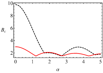
Figure 2: The dashed black line shows the critical field $B_{c}$ as a function of the ratio $\alpha=\Gamma_{x}/\omega$ for the AC driven Ising system coupled to a $7/2$ spin bath. The red solid line corresponds to the AC driven system in absence of the spin bath. At low amplitude, the spin bath contributes very strongly and drastically changes the critical field due to the blocking mechanism. As the amplitude increases, the effect of the bath is removed and only the transverse part $A_{0}^{x}$ contributes with a small shift. There are some regions where $B_{c}$ in presence of a bath is even lower than in the absence of hyperfine coupling ($\alpha\sim 1.7-2.7$). These are the regions where $\tilde{A}_{0}^{y,z}$ changes sign and overcomes $A_{0}^{x}$. The parameters are fixed according to the experimental ones for $LiHoF_{4}$:$V_{0}^{zz}=6$ K, $A_{0}^{z}=0.2$ K and $A_{0}^{x,y}=0.02$ K.

This plot shows that for small $\alpha$, the system behaves as in the undriven case, where the spin bath greatly affects the value of the critical field due to the blocking mechanism. As this blocking is produced by the difference between the transverse $A_{0}^{x}$ and the longitudinal hyperfine coupling $A_{0}^{y,z}$, and the later is renormalized by the AC field, one can observe that by increasing $\alpha$ the system approaches the isolated system behavior. Therefore it would be possible to experimentally analyze the opposite regimes of ideal Ising QPT in absence and in presence of a spin bath by just tuning the external AC field.

As we previously pointed out, it is important to discuss the effect of the high frequency corrections neglected in the Magnus expansion (Eq.7). We have calculated the next order leading term $\frac{1}{2\omega^{2}}\sum_{n=1}^{\infty}\frac{1}{n^{2}}\left(\left[\left[\tilde{H}_{n},\tilde{H}_{0}\right],\tilde{H}_{-n}\right]+h.c.\right)$, and although the effective Hamiltonian contains now up to four-body interactions, they are all weighted by Bessel functions and a factor $\omega^{-2}$, which in general give corrections one or two orders of magnitude smaller than $\tilde{H}_{0}$. Importantly, we find that the transverse blocking mechanism, produced due to the initially large anisotropy between $A_{0}^{z}$ and $A_{0}^{x,y}$, is not restored by the second order corrections, and the renormalized critical point should not be greatly affected. Nevertheless one should be careful with the growth of high frequency corrections for large times; this would restrict the maximum duration of the experiments to times shorter than the inverse of the energy correction. In addition, the time control can be complex due to the competition between the initialization time and the infinite temperature limit of interacting Floquet systemsInfinite-temperature , but several strategies based on the properties of the transient dynamics could allow to overcome this issueThermalization ; Floquet-MBL . As a check we have included in the Appendix the simulation of the dynamics of the Quantum Ising system coupled to a spin bath, when the QCP is crossed from the ferromagnetic phase. It shows that in absence of the AC field, the QPT to the paramagnetic phase is suppressed due to the spin bath, but in the presence of the AC field tuned to $\mathcal{J}_{0}\left(\alpha\right)=0$, the time average magnetization $\int_{0}^{T}M_{z}\left(t\right)dt$ vanishes, indicating the cancellation of the longitudinal hyperfine coupling $\tilde{\mathcal{A}}_{0}^{z}=0$. Therefore, one can conclude that the high frequency corrections do not affect the suppression of the hyperfine interaction, at least within the time scales of the simulation.

VI Concluding remarks

We have obtained a static effective Hamiltonian for the AC driven transverse Ising model in the presence of a spin bath, in which the inter-spin and the hyperfine interactions are renormalized as a function of the AC field intensity and frequency. We have found that the inter-spin and hyperfine interaction renormalize differently, which allows to study the Ising QPT in a large number of cases ranging from positive to negative hyperfine interaction (Fig.2). The effective Hamiltonian for the AC driven Quantum Ising model in Eq.8, and the effective hyperfine interaction in Eq.15 are general results, valid in arbitrary dimension; however the magnetization in Eq.16 is calculated to lowest order and should be more accurate for higher dimensional systems such as the 3D Quantum Ising model. Importantly, the equations for the magnetization in the presence of the spin bath are derived for arbitrary large spins, which allows to apply this theory to different types of spin bath. Finally, the phase diagram in Eq.1 is obtained as a function of the transverse field and the temperature $T=1/\beta$, which is in general ill-defined for non-equilibrium situations such as the one with the AC field. The temperature is set by a phonon bath, and in order to avoid heating due to the AC field, a pulsed field experiment would be useful, with the pulses short enough so that the spin-phonon couplings have no time to heat the phonon bath. As we previously discussed, the initialization protocol should be engineered so as to reach the desired steady state, which can be done using adiabatic launching. Furthermore, in some cases the interactions with the phonon bath could be used to stabilize the steady statePopulation-Floquet

The classic QPT magnetic insulator $LiHo_{x}Y_{1-x}F_{4}$, with spin $S=8$ magnetic ions, perhaps the canonical Quantum Ising system, displays quantum annealing Qanneal and a quantum spin glass phase QSpGl , as well as quantum critical behavior Qcrit . However, the strong coupling to the nuclear spin bath disrupts completely the expected quantum critical behavior around the QCP aeppli05 ; schechter05 (and leads to various other dynamic and thermodynamic effects giraud ; luke10 ; kycia-dyn ). For nearest neighbor spins, $|V_{i,j}|\rightarrow V\sim 1.2x$, in K units, and the hyperfine level splitting $|A|\sim 0.22$K (with spin $I=7/2$). In a high frequency AC field ($\Lambda_{o}\gg\hbar\omega\gg|V_{i,j}|,|A_{r,j}^{\mu}|$, ie, for $\omega\sim 30-200$ GHz), we may then directly apply the theory given here. The results are shown in Figs. 1 and 2), and these constitute predictions for this system.

In the $Fe_{8}$ system the hyperfine couplings are much smaller, and can be varied by isotopic substitutionWW00 . Because there is a whole spectrum of these couplings, one cannot suppress them all simultaneously - but one can select out particular groups of nuclear spins for suppression, and the effective couplings as a function of applied field are well understood MST06 ; takahashi . What is interesting here is the possibility of controlling the longitudinal dipolar coupling between molecules, allowing one to look at single molecule dynamics.

In ion trap spin chains we can typically discount spin bath effects. What is interesting here is the possibility of varying the range of the inter-spin interactions, as well as their strength, and observing the spin dynamics in real time for both short- and long-range interaction forms ionChain2 ; calculations including corrections to the RPA result are underway to give quantitative predictions, as they can be important for low dimensional systems. In these systems one can also introduce transverse inter-spin interactions - this makes the eventual phase diagram very rich indeed.

In all three systems experimental testing of the results herein should be easily possible - quantitative comparison will require numerical work, and we emphasize that in real experiments one will need to take account of demagnetization fields, which are in general inhomogeneous in real systems. This will need to be evaluated numerically (compare takahashi ), and experiments with “whisker”-shaped samples (for solid-state systems) would be useful.

This work has been supported by NSERC of Canada, and by PITP. We acknowledge helpful discussions with G. Aeppli on the experimental constraints.

Appendix A Magnus expansion

To quantify the renormalization effects produced by a large amplitude of the AC field, one must first use a transformation to the interaction picture:

$$\tilde{H}\left(t\right)=U_{1}H\left(t\right)U_{1}^{\dagger}-iU_{1}\dot{U}_{1}^{\dagger}=-\sum_{i}\Delta_{o}\tilde{\tau}_{i}^{x}-\frac{1}{2}\sum_{i,j\neq i}V_{i,j}\tilde{\tau}_{i}^{z}\tilde{\tau}_{j}^{z}+\sum_{\mu,r,j}A_{r,j}^{\mu}I_{r}^{\mu}\tilde{\tau}_{j}^{\mu}$$ (18)

where $U_{1}=\exp\left[i\int\sum_{j}\Gamma\left(t\right)\tau_{j}^{x}\right]dt$, with $\mu=x,y,z$ and $\tilde{\tau}_{j}^{\mu}\equiv U_{1}\tau_{j}^{\mu}U_{1}^{\dagger}$. For the calculation of the Magnus expansion one needs the Fourier coefficients of the time dependent Hamiltonian. They are given by the next expressions:

$$\tilde{H}_{0}=-\sum_{i}\Delta_{o}\tau_{i}^{x}-\sum_{i,j\neq i}\frac{V_{i,j}}{4}\left\{\left[1+\mathcal{J}_{0}\left(2\alpha\right)\right]\tau_{i}^{z}\tau_{j}^{z}+\left[1-\mathcal{J}_{0}\left(2\alpha\right)\right]\tau_{i}^{y}\tau_{j}^{y}\right\}+\sum_{\mu,r,j}\tilde{A}_{r,j}^{\mu}I_{r}^{\mu}\tau_{j}^{\mu}$$ (19)

$$\tilde{H}_{\pm\left(2n+1\right)} = \pm i\sum_{i,j\neq i}\frac{V_{ij}\mathcal{J}_{2n+1}\left(2\alpha\right)}{4}\left(\tau_{i}^{y}\tau_{j}^{z}+\tau_{i}^{z}\tau_{j}^{y}\right)\pm i\mathcal{J}_{2n+1}\left(\alpha\right)\sum_{r,j}\left(A_{r,j}^{y}I_{r}^{y}\tau_{j}^{z}-A_{r,j}^{z}I_{r}^{z}\tau_{j}^{y}\right)$$ (20)

$$\tilde{H}_{\pm 2\left(n+1\right)} = -\sum_{i,j\neq i}\frac{V_{ij}\mathcal{J}_{2n+2}\left(2\alpha\right)}{4}\left(\tau_{i}^{z}\tau_{j}^{z}-S_{i}^{y}\tau_{j}^{y}\right)+\mathcal{J}_{2\left(n+1\right)}\left(\alpha\right)\sum_{r,j}\left(A_{r,j}^{y}I_{r}^{y}\tau_{j}^{y}+A_{r,j}^{z}I_{r}^{z}\tau_{j}^{z}\right)$$ (21)

where $\alpha\equiv\Gamma_{x}/\omega$, $\mathcal{J}_{m}\left(\alpha\right)$ is an $m$-th order Bessel function, and where the renormalized hyperfine couplings are

$$\tilde{A}_{r,j}^{x}=A_{r,j}^{x},\quad\tilde{A}_{r,j}^{y}=A_{r,j}^{y}\mathcal{J}_{0}\left(\alpha\right),\quad\tilde{A}_{r,j}^{z}=A_{r,j}^{z}\mathcal{J}_{0}\left(\alpha\right).$$ (22)

From these expression we see that $\left[\tilde{H}_{n},\tilde{H}_{-n}\right]=0$, and to order $1/\omega$ we only need to use $\tilde{H}_{0}$ in the expansion. The effective time-independent Hamiltonian becomes:

$$\mathcal{H} = -\sum_{i}\Delta_{o}\tau_{i}^{x}-\frac{1}{2}\sum_{i,j\neq i}^{N}\left[\tilde{V}_{ij}^{zz}\tau_{i}^{z}\tau_{j}^{z}+\tilde{V}_{ij}^{yy}\tau_{i}^{y}\tau_{j}^{y}\right]+\sum_{\mu,r,j}\tilde{A}_{r,j}^{\mu}I_{r}^{\mu}\tau_{j}^{\mu}$$ (23)

in which the renormalized couplings are:

$$\tilde{V}_{i,j}^{zz}\left(\alpha\right) = V_{i,j}\left[1+\mathcal{J}_{0}\left(2\alpha\right)\right]/2$$ (24)

$$\tilde{V}_{ij}^{yy}\left(\alpha\right) = V_{i,j}\left[1-\mathcal{J}_{0}\left(2\alpha\right)\right]/2$$ (25)

We see that under the effect of the AC field the model becomes an effective anisotropic ”$XY$” (actually, $YZ$) spin system in a transverse field. Thus one effect of the AC field is to modify the very strong dominance of the ”zz” coupling in the effective dipolar interaction between Ising spins. We note also that the argument of the Bessel functions in the renormalized hyperfine couplings is half that involved in the renormalized inter-spin couplings.

Appendix B Magnetization calculation

Here we include the details of the calculation for the magnetization self-consistency equations in presence of the spin bath. A more general form of the Hamiltonian discussed in this paper is:

$$H=-\sum_{\mu,j}B_{\mu}S_{j}^{\mu}-\frac{1}{2}\sum_{\mu}\sum_{j,l\neq j}V_{j,l}^{\mu}S_{j}^{\mu}S_{l}^{\mu}+\sum_{\mu,r,j}A_{r,j}^{\mu}I_{r}^{\mu}S_{j}^{\mu}$$ (26)

where $\alpha,\beta=x,y,z$, and $S_{n}^{\alpha}$ operates on an arbitrary spin of spin S (not just $S=1/2$) at site $n$; the nuclear spin $I_{r}^{\mu}$ also takes arbitrary value. We are interested in the Green’s function for the calculation of the magnetization, defined by:

$$G_{n,m}^{\alpha,\beta}\left(t,t^{\prime}\right)=-i\langle S_{n}^{\alpha}\left(t\right);S_{m}^{\beta}\left(t^{\prime}\right)\rangle$$ (27)

where $\langle\ldots\rangle$ corresponds to the statistical average with respect to the thermal density matrix $\rho=e^{-\beta H}$, and the semi-colon indicates that we can consider the time ordered, retarded or advanced Green’s functions (they all have the same equation of motion). The corresponding equation of motion for the electronic spins is given by:

$$\omega G_{n,m}^{\alpha,\beta}\left(\omega\right) =\frac{1}{2\pi}\langle\left\{S_{n}^{\alpha},S_{m}^{\beta}\right\}\rangle+i\sum_{\mu}\epsilon_{\mu\alpha\delta}B_{\mu}G_{n,m}^{\delta,\beta}\left(\omega\right)$$ (28)

$$+i\sum_{\mu}\epsilon_{\mu\alpha\delta}\sum_{j\neq n}V_{n,j}^{\mu}G_{jn,m}^{\mu\delta,\beta}\left(\omega\right)-i\sum_{\mu,r}\epsilon_{\mu\alpha\delta}A_{r,n}^{\mu}K_{rn,m}^{\mu\delta,\beta}\left(\omega\right)$$

where we have defined:

$$G_{jn,m}^{\mu\delta,\beta}\left(t,t^{\prime}\right)=-i\langle S_{j}^{\mu}\left(t\right)S_{n}^{\delta}\left(t\right);S_{m}^{\beta}\left(t^{\prime}\right)\rangle,\quad K_{rn,m}^{\mu\delta,\beta}\left(t,t^{\prime}\right)=-i\langle I_{r}^{\mu}\left(t\right)S_{n}^{\delta}\left(t\right);S_{m}^{\beta}\left(t^{\prime}\right)\rangle$$ (29)

The expression above is valid for arbitrary spin values. Note that we have used anti-commutation relationships for the definition of the Green’s functions, as it is more convenient for the underlying pole structure that we will encounter later on. In what follows we adapt the spin operator decoupling methods discussed by, eg., Wang et al. Fermion-GF , for lattice electronic spins, to the more general case of a set of lattice spins coupled to nuclear spins.

We decouple the higher Green functions in the equation of motion neglecting correlations between different sites. This approximation can be understood from the perspective of a $1/Z$ expansion, being $Z$ the coordination number of the system. It is known that to lowest order, ie neglecting quantum correlations, the $1/Z$ expansion agrees with the Random Phase Approximation (RPA) and that for higher dimensional systems such as the 3D Ising model considered for $LiHoF$, it should provide reasonable good resultsRonnowPRB ; aeppli05 . Once applied the decoupling scheme, we find:

$$\omega G_{n,n}^{\alpha,\beta} =\frac{\chi_{\alpha,\beta}}{2\pi}+i\sum_{\mu}\epsilon_{\mu\alpha\delta}\left(B_{\mu}+\sum_{j\neq n}V_{n,j}^{\mu}\langle S_{j}^{\mu}\rangle-\sum_{r}A_{r,n}^{\mu}\langle I_{r}^{\mu}\rangle\right)G_{n,n}^{\delta,\beta}$$ (30)

where $\chi_{\alpha\beta}=\langle\left\{S_{n}^{\alpha},S_{n}^{\beta}\right\}\rangle$ are the spin anti-commutators (we suppress the site index $n$) and $G_{n,n}^{\alpha,\beta}$ is now the Green’s function in the RPA approximation. The calculation of the Green’s functions is fairly straightforward Fermion-GF ); we rewrite the system of equations as:

$$\left(\boldsymbol{1}\omega-\boldsymbol{H}\right)\boldsymbol{G}\left(\omega\right)=\boldsymbol{F},\ \boldsymbol{G}\left(\omega\right)=\left(\begin{array}[]{c}G_{n,n}^{x,\beta}\left(\omega\right)\\ G_{n,n}^{y,\beta}\left(\omega\right)\\ G_{n,n}^{z,\beta}\left(\omega\right)\end{array}\right)$$ (31)

where

$$\boldsymbol{F}=\frac{1}{2\pi}\left(\begin{array}[]{c}\chi_{x,\beta}\\ \chi_{y,\beta}\\ \chi_{z,\beta}\end{array}\right),\ \boldsymbol{H}=\left(\begin{array}[]{ccc}0&iH_{z}&-iH_{y}\\ -iH_{z}&0&iH_{x}\\ iH_{y}&-iH_{x}&0\end{array}\right),$$ (32)

and $H_{\alpha}$ are the components of an effective field defined as

$$H_{\alpha}=B_{\alpha}+M_{\alpha}V_{0}^{\alpha}-m_{\alpha}A_{\alpha},$$ (33)

$M_{\alpha}$ is the electronic spin magnetization, and $m_{\alpha}$ the nuclear spin bath magnetization. The $\boldsymbol{H}$ matrix can be diagonalized and has eigenvalues $\omega=\left\{0,\pm\sqrt{\sum_{\alpha}H_{\alpha}^{2}}\right\}$.

The Green’s functions can be obtained as:

$$G_{n,n}^{\alpha,\beta}=\sum_{\lambda=1}^{3}\sum_{\tau=1}^{3}\frac{U_{\alpha\tau}U_{\tau\lambda}^{-1}}{\omega-\omega_{\tau}}F^{\lambda,\beta}=\sum_{\lambda=1}^{3}R^{\alpha,\lambda}F^{\lambda,\beta}$$ (34)

where $U$ is the matrix that diagonalizes $\boldsymbol{H}$. From this expression we calculate the statistical averages straightforwardly using:

$$\langle S_{n}^{\beta}S_{n}^{\alpha}\rangle=i\int\frac{G_{n,n}^{\alpha,\beta}\left(\omega+i\epsilon\right)-G_{n,n}^{\alpha,\beta}\left(\omega-i\epsilon\right)}{e^{\beta\omega}+1}d\omega$$ (35)

$$\langle S_{n}^{\beta}S_{n}^{\alpha}\rangle=\sum_{\lambda=1}^{3}\sum_{\tau=1}^{3}\frac{U_{\alpha\tau}U_{\tau\lambda}^{-1}}{e^{\beta\omega_{\tau}}+1}\tilde{F}^{\lambda,\beta}$$ (36)

where

$$\tilde{F}^{\lambda\beta}=2\pi F^{\lambda\beta}=\chi^{\lambda\beta}$$ (37)

In order to simplify the expression we can use the relation between commutators and anti-commutators:

$$\langle\left\{S_{n}^{\alpha},S_{n}^{\beta}\right\}\rangle = \langle\left[S_{n}^{\alpha},S_{n}^{\beta}\right]\rangle+2\langle S_{n}^{\beta}S_{n}^{\alpha}\rangle$$ (38)

Writing $\Gamma=\sum_{\tau=1}^{3}\frac{U_{\alpha\tau}U_{\tau\lambda}^{-1}}{e^{\beta\omega_{\tau}}+1}$, the matrix equation for the statistical averages becomes:

$$\left(\boldsymbol{1}-2\boldsymbol{\Gamma}\right)\left(\begin{array}[]{c}\langle S_{n}^{\beta}S_{n}^{x}\rangle\\ \langle S_{n}^{\beta}S_{n}^{y}\rangle\\ \langle S_{n}^{\beta}S_{n}^{z}\rangle\end{array}\right) = \boldsymbol{\Gamma}\left(\begin{array}[]{c}\langle\left[S_{n}^{\alpha},S_{n}^{\beta}\right]\rangle\\ \langle\left[S_{n}^{\alpha},S_{n}^{\beta}\right]\rangle\\ \langle\left[S_{n}^{\alpha},S_{n}^{\beta}\right]\rangle\end{array}\right)$$ (45)

We now define everything in terms of a dimensionless ”eigenvalue normalized” effective field $h_{\alpha}=H_{\alpha}/\sqrt{\sum_{\alpha}H_{\alpha}^{2}}$, and a renormalized frequency $\tilde{\omega}=\omega/\sqrt{\sum_{\alpha}H_{\alpha}^{2}}$. The explicit calculation of the matrix equation results in:

$$2\left(\begin{array}[]{ccc}0&ih_{z}&-ih_{y}\\ -ih_{z}&0&ih_{x}\\ ih_{y}&-ih_{x}&0\end{array}\right)\left(\begin{array}[]{c}\langle S_{n}^{\beta}S_{n}^{x}\rangle\\ \langle S_{n}^{\beta}S_{n}^{y}\rangle\\ \langle S_{n}^{\beta}S_{n}^{z}\rangle\end{array}\right)=\left(\begin{array}[]{ccc}\coth\left(\frac{\beta\tilde{\omega}}{2}\right)&-ih_{z}&ih_{y}\\ ih_{z}&\coth\left(\frac{\beta\tilde{\omega}}{2}\right)&-ih_{x}\\ -ih_{y}&ih_{x}&\coth\left(\frac{\beta\tilde{\omega}}{2}\right)\end{array}\right)\left(\begin{array}[]{c}i\epsilon_{x\beta\delta}\langle S_{n}^{\delta}\rangle\\ i\epsilon_{y\beta\delta}\langle S_{n}^{\delta}\rangle\\ i\epsilon_{z\beta\delta}\langle S_{n}^{\delta}\rangle\end{array}\right)$$ (46)

In order to solve these coupled equations one must realize that they are not independent, as the determinant of $\boldsymbol{I}-2\boldsymbol{\Gamma}$ vanishes. The first row multiplied by $h_{x}$, plus the second row times $h_{y}$, plus the third row times $h_{z}$ gives zero. The same condition on the right reads:

$$\epsilon_{x\beta\delta}\langle S_{n}^{\delta}\rangle h_{x}+\epsilon_{y\beta\delta}\langle S_{n}^{\delta}\rangle h_{y}+\epsilon_{z\beta\delta}\langle S_{n}^{\delta}\rangle h_{z}=0$$ (47)

If we now choose $\beta=x,y,z$ we find, respectively:

$$\langle S_{n}^{y}\rangle h_{z} =\langle S_{n}^{z}\rangle h_{y}$$

$$\langle S_{n}^{z}\rangle h_{x} =\langle S_{n}^{x}\rangle h_{z}$$

$$\langle S_{n}^{x}\rangle h_{y} =\langle S_{n}^{y}\rangle h_{x}$$

which are the so called regularity conditions. They imply that we only need to know one of the components of the magnetization in order to calculate the other components.

Actually one can solve a somewhat more general system of equations, again for arbitrary spin. Consider an arbitrary polynomial function of spin operators of form:

$$P\left(\left\{S_{n}^{\alpha}\right\}\right) = \sum_{r,p,q=1}^{2S+1}c_{rpq}\left(S_{n}^{x}\right)^{r}\left(S_{n}^{y}\right)^{p}\left(S_{n}^{z}\right)^{q}$$ (48)

then we have the equation:

$$\left(\begin{array}[]{ccc}0&ih_{z}&-ih_{y}\\ -ih_{z}&0&ih_{x}\\ ih_{y}&-ih_{x}&0\end{array}\right)\left(\begin{array}[]{c}\langle P_{n}S_{n}^{x}\rangle\\ \langle P_{n}S_{n}^{y}\rangle\\ \langle P_{n}S_{n}^{z}\rangle\end{array}\right)=\frac{1}{2}\left(\begin{array}[]{ccc}\coth\left(\frac{\beta\tilde{\omega}}{2}\right)&-ih_{z}&ih_{y}\\ ih_{z}&\coth\left(\frac{\beta\tilde{\omega}}{2}\right)&-ih_{x}\\ -ih_{y}&ih_{x}&\coth\left(\frac{\beta\tilde{\omega}}{2}\right)\end{array}\right)\left(\begin{array}[]{c}\langle\left[S_{n}^{x},P_{n}\right]\rangle\\ \langle\left[S_{n}^{y},P_{n}\right]\rangle\\ \langle\left[S_{n}^{z},P_{n}\right]\rangle\end{array}\right)$$

If we take this set of equations for $P_{n}\equiv P\left(\left\{S_{n}^{\alpha}\right\}\right)$, along with the regularity conditions

$$\left(S_{n}^{x}\right)^{2}+\left(S_{n}^{y}\right)^{2}+\left(S_{n}^{z}\right)^{2} =S\left(S+1\right)$$ (49)

$$\left[S_{n}^{\alpha},S_{n}^{\beta}\right] =i\epsilon_{\alpha\beta\delta}S_{n}^{\delta}$$ (50)

$$\langle S_{n}^{z}\rangle h_{x}=\langle S_{n}^{x}\rangle h_{z},\ \langle S_{n}^{x}\rangle h_{y}=\langle S_{n}^{y}\rangle h_{x},\ \langle S_{n}^{y}\rangle h_{z} =\langle S_{n}^{z}\rangle h_{y}$$ (51)

and the usual spin algebra identities for spin-$S$ degrees of freedom, we find that the system of equations for the two-point functions $\langle S_{n}^{\beta}S_{n}^{\alpha}\rangle$ and $\langle S_{n}^{x,y}\rangle$ can be solved as a function of $\langle S_{n}^{z}\rangle$, i.e., we need one extra equation to solve the system. This can be obtained from the identity:

$$\prod_{r=-S}^{S}\left(S_{n}^{z}-r\right)=0$$ (52)

which clearly becomes more and more complicated as the spin $S$ is increased.

Specific Cases involving electronic and nuclear spins: As a first check, we can take $S=1/2$. In that case we find that $\left(S_{n}^{z}\right)^{2}=1/4$, which provides the extra equation needed for the solution. The system of equations results in:

$$\langle S_{n}^{\mu}\rangle=\frac{h_{\mu}}{2}\tanh\left(\frac{\beta\tilde{\omega}}{2}\right),\ \langle\left(S_{n}^{\mu}\right)^{2}\rangle=\frac{1}{4},\ \langle S_{n}^{\mu}S_{n}^{\nu}\rangle=i\frac{\epsilon_{\mu\nu\delta}h_{\delta}}{4}\tanh\left(\frac{\beta\tilde{\omega}}{2}\right)$$ (53)

which is the expected result from the RPA calculation for a spin $1/2$.

Consider now the case of $S=1$, for which the extra equation reads:

$$\left(S_{n}^{z}\right)^{3}=S_{n}^{z}$$ (54)

Hence, we must obtain statistical averages for $\left(S_{n}^{z}\right)^{3}$ as well by setting $P_{n}=\left(S_{n}^{x}\right)^{p}\left(S_{n}^{y}\right)^{q}\left(S_{n}^{z}\right)^{r}$ (for this case $p,q,r=0,1,2$ is sufficient) and solving for a larger system of equations. We can then see how a general rule for arbitrary spins emerges - this was derived by Wang et al. Fermion-GF - and one finds:

$$\langle S_{n}^{z}\rangle=\frac{\left[\left(2S+1\right)R-Q_{z}\right]\left(Q_{z}+R\right)^{2S+1}+\left[\left(2S+1\right)R+Q_{z}\right]\left(Q_{z}-R\right)^{2S+1}}{2R^{2}\left[\left(Q_{z}+R\right)^{2S+1}-\left(Q_{z}-R\right)^{2S+1}\right]}$$ (55)

where we have defined

$$R=1/\left|h_{z}\right|,\ Q_{z}=\frac{\coth\left(\frac{\beta\tilde{\omega}}{2}\right)}{h_{z}}$$ (56)

Now it is easy to see how to deal with a set of coupled nuclear and electronic spins. We first consider the nuclear spin averages. As an example, take the case where $I_{n}=7/2$ (the case of the $Ho$ nuclear spins in the $LiHoF$ system). Then for the nuclear spin averages we get

$$\langle I_{n}^{z}\rangle =\frac{1}{2Q_{z}}+\frac{2Q_{z}}{Q_{z}^{2}+R^{2}}+\frac{8Q_{z}\left(Q_{z}^{2}+R^{2}\right)}{Q_{z}^{4}+6Q_{z}^{2}R^{2}+R^{4}}$$ (57)

$$\langle I_{n}^{y}\rangle =\frac{h_{y}}{h_{z}}\langle I_{n}^{z}\rangle,\ \langle I_{n}^{x}\rangle=\frac{h_{x}}{h_{z}}\langle I_{n}^{z}\rangle$$ (58)

As these equations depend on $\tilde{\omega}=\tilde{\omega}\left(\langle I_{n}^{x}\rangle,\langle I_{n}^{y}\rangle,\langle I_{n}^{z}\rangle\right)$, we have to solve them numerically.

If we now consider the full $LiHo$ system, ie., with a coupling between an Ising electronic system ($S=1/2$) and a spin bath ($I=7/2$), the self-consistency equations are coupled for all values of the magnetization. We then find:

$$M_{\mu} =\frac{h_{\mu}^{S}}{2}\tanh\left(\frac{\beta\tilde{\omega}}{2}\right)$$ (59)

$$m_{\mu} =\frac{h_{z}^{B}}{2}\left[\tanh\left(\frac{\beta\tilde{\Omega}}{2}\right)+2\tanh\left(\beta\tilde{\Omega}\right)+4\tanh\left(2\beta\tilde{\Omega}\right)\right]$$

for the electronic system and nuclear bath magnetization respectively, where $h_{\mu}^{S\left(B\right)}=H_{\mu}^{S\left(B\right)}/\tilde{\omega}\left(\tilde{\Omega}\right)$ represent the system(environment) normalized fields respectively, and $\tilde{\omega}\left(\tilde{\Omega}\right)$ represent the normalized eigenenergies of the system(environment) respectively. Note that now $h_{\mu}^{S}=h_{\mu}^{S}\left(M_{\mu},m_{\mu}\right)$, $h_{\mu}^{B}=h_{\mu}^{B}\left(M_{\mu}\right)$, $\tilde{\Omega}=\tilde{\Omega}\left(M_{\mu}\right)$ and $\tilde{\omega}=\tilde{\omega}\left(M_{\mu},m_{\mu}\right)$. We can easily obtain the $T=0$ limit from these expressions; we get:

$$M_{\mu} =\frac{1}{2}\frac{B_{\mu}+M_{\mu}V_{0}^{\mu}-A_{0}^{\mu}m_{\mu}}{\sqrt{\left(B_{x}-A_{0}^{x}m_{x}\right)^{2}+A_{0}^{y}m_{y}^{2}+\left(V_{0}^{z}M_{z}-A_{0}^{z}m_{z}\right)^{2}}}$$ (60)

$$m_{\mu} =-\frac{7}{2}\frac{A_{\mu}M_{\mu}}{\sqrt{\left(A_{0}^{x}M_{x}\right)^{2}+\left(A_{0}^{y}M_{y}\right)^{2}+\left(A_{0}^{z}M_{z}\right)^{2}}}$$ (61)

We can directly substitute $m_{\mu}$ into the system’s magnetization. Since we are interested in the behavior at large $B_{x}$, in order to see if the QPT can be blocked, we note that in the asymptotic limit $B_{x}\gg A_{\mu},V_{0}^{z}$, one finds:

$$M_{x}\lesssim\frac{1}{2},\ M_{z}\simeq\frac{m_{z}V_{0}^{z}}{2B_{x}}+\frac{7\left(A_{0}^{z}\right)^{2}m_{z}}{4B_{x}\sqrt{\left(A_{0}^{x}m_{x}\right)^{2}+\left(A_{0}^{z}m_{z}\right)^{2}}}$$ (62)

Clearly in the second equation we could have $M_{z}=0$ as a solution of the system, meaning that a QPT would exist. However, if we assume the highly anisotropic case $A_{z}\neq 0$, $A_{x}=0$, we find:

$$M_{z}=\frac{1}{2}\frac{M_{z}V_{0}^{z}+\frac{7}{2}A_{0}^{z}}{\sqrt{B_{x}^{2}+\left(V_{0}^{z}M_{z}+\frac{7}{2}A_{0}^{z}\right)^{2}}}\simeq\frac{M_{z}V_{0}^{z}}{2B_{x}}+\frac{7A_{0}^{z}}{4B_{x}}$$ (63)

which proves that $M_{z}$ will always have a remnant magnetization blocking the QPT at $T=0$ for all $B_{x}$ (the second equation can never be fulfilled when $M_{z}=0$). Hence, the longitudinal hyperfine coupling blocks the phase transition as one would expect.

Appendix C Dynamics across the quantum critical point

Here we include simulations of the magnetization dynamics for the Quantum Ising model coupled to a spin bath when it crosses a QCP. The simulation is performed for a slightly simpler version of the Ising model than the one considered in the main text, but the differences should not be important for the final conclusions. We consider a finite Ising system coupled to a spin bath made of $\frac{1}{2}$-spins (we assumed $I=1/2$ instead of $I=7/2$ for simplicity, but the renormalization of the hyperfine coupling should make no difference between the two). We then integrate numerically over time the Heisenberg equation of motion under the same decoupling scheme used for the calculation of the Green’s functions. Fig.3(left) shows the case without AC field and hyperfine coupling, as a test for the protocol. As the transverse DC field increases, the longitudinal magnetization decreases, vanishing when $B=B_{c}$. The small oscillations around the mean value $M_{z}=0$ correspond to non-adiabatic effects during the protocol. Fig.3(right) corresponds to the case with hyperfine coupling, where the QPT is suppressed due to the transverse blocking mechanism and a remnant magnetization is always present. Finally, the case with AC field and hyperfine coupling is not explicitly shown due to the fast oscillations of the magnetization, but we find that the average value of the longitudinal magnetization is $\int_{0}^{T}M_{z}\left(t\right)dt\simeq 0.0003$ for $\mathcal{J}_{0}\left(\alpha\right)=0$ and frequency $\omega=10V_{i,j}$. This indicates that the renormalization of the longitudinal hyperfine coupling persists when all corrections to the Magnus expansion are included, and it is even possible to adiabatically cross the QCP.

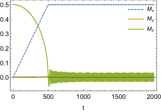
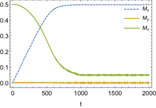
Figure 3: (Left) Magnetization as a function of time for the Quantum Ising model in absence of AC field and hyperfine coupling. During the protocol, the transverse magnetic field increases linearly to its final value $B_{x}=2B_{c}$ at $t=1000$. At $t=500$ the system crosses the QCP and non-adiabatic effects produce the oscillations that persist at large times (which average to $M_{z}=0$ indicating the presence of the PM phase). (Right) Simulation in the presence of hyperfine coupling, where the magnetization remains finite due to the transverse blocking mechanism, indicating the absence of QPT to the PM phase. Time is measured in inverse units of $V_{i,j}$.

References

- (1) J.A. Hertz, Phys. Rev. B 14, 1165 (1976).
- (2) N.V. Prokof’ev, PCE Stamp, Rep. Prog. Phys. 63, 669 (2000).
- (3) H.M. Ronnow et al., Science 308, 389 (2005).
- (4) H.M. Ronnow et al., Phys. Rev. B 75, 054426 (2007).
- (5) L. Viola, E. Knill, and S. Lloyd, Phys. Rev. Lett. 82, 2417 (1999).
- (6) W. Zhang, N. P. Konstantinidis, V. V. Dobrovitski, B. N. Harmon, L. F. Santos, and L. Viola, Phys. Rev. B 77, 125336 (2008).
- (7) G. de Lange, Z. H. Wang, D. Riste, V. V. Dobrovitski and R. Hanson, Science 330, 60 (2010).
- (8) G. de Lange, T. van der Sar, M. Blok, Z.-H. Wang, V. Dobrovitski and R. Hanson, Scientific Reports 2, 382 (2012).
- (9) N. Bar-Gill, L.M. Pham, C. Belthangady, D. Le Sage, P. Cappellaro, J.R. Maze, M.D. Lukin, A. Yacoby and R. Walsworth, Nature Communications 3, 858 (2012).
- (10) M. Schechter, PCE Stamp, Phys. Rev. Lett. 95, 267208 (2005); and Phys. Rev. B 78, 054438 (2008).
- (11) J. Brooke, D Bitko, T.F. Rosenbaum, G. Aeppli, Science 284, 779 (1999).
- (12) A. Dutta, G. Aeppli, B. K. Chakrabarti, U. Divakaran, T. F. Rosenbaum and D. Sen, Quantum Phase Transitions in Transverse Field Spin Models: From Statistical Physics to Quantum Information (Cambridge University Press, Cambridge, 2015)
- (13) TF Rosenbaum, J. Phys. Cond. Mat. 8, 9759 (1996); PE Jonsson et al., Phys. Rev. Lett. 98, 256403 (2007); C Ancona-Torres, DM Silevitch, G Aeppli, TF Rosenbaum, Phys. Rev. Lett. 101, 057201 (2008); JA Quilliam et al., Phys. Rev. Lett. 101, 187204 (2008); and MA Schmidt et al., PNAS 111, 3689 (2014).
- (14) D. Bitko, T.F. Rosenbaum, G. Aeppli, Phys. Rev. Lett. 77, 940 (1996); J.A. Quilliam et al., Phys. Rev. Lett. 98, 037203 (2007), and refs. therein.
- (15) R. Giraud et al., Phys. Rev. Lett. 81, 057203 (2001); R Giraud, A.M. Tkachuk, B. Barbara, Phys. Rev. Lett. 91, 257204 (2003)
- (16) J. Rodriguez et al., Phys. Rev. Lett. 105, 107203 (2010); RC Johnson et al., Phys. Rev. B 86, 014427 (2012)
- (17) S. Ghosh et al., Science 296, 2195 (2002), and Nature 425, 48 (2003); JA Quilliam, S Meng, JB Kycia, Phys. Rev. Lett. B 85, 184415 (2012)
- (18) W. Wernsdorfer and R. Sessoli, Science 284, 133 (1999); W. Wernsdorfer et al., Phys. Rev. Lett. 84, 2965 (2000).
- (19) A. Morello, P.C.E. Stamp, P. C. E. & I.S. Tupitsyn, Phys. Rev. Lett. 97, 207206 (2006).
- (20) S. Takahashi et al., Nature 476, 76 (2011)
- (21) K. Kim, Phys. Rev. Lett. 103, 120502 (2009); J.W. Britton et al., Nature 484, 489 (2012); R. Islam et al., Science 340, 583 (2013).
- (22) P. Richerme et al., Nature 511, 198 (2014); P. Jurcevic et al., Nature 511, 202 (2014). See also J.G Bohnet et al., arXiv:1512.03576 (2015).
- (23) J.G. Bohnet et al., arXiv:1512.03576 (2015).
- (24) J. Jensen, A. MacKintosh, ”Rare Earth Magnetism” (Clarendon, Oxford, 1991).
- (25) A.L. Barra, D. Gatteschi, D. & R. Sessoli, Chem. Eur. J. 6, 1608 (2000).
- (26) V. M. Bastidas, C. Emary, G. Schaller, and T. Brandes Phys. Rev. A 86, 063627 (2012).
- (27) Tony E. Lee, Yogesh N. Joglekar, and Philip Richerme Phys. Rev. A 94, 023610 (2016).
- (28) N. Lindner, G. Rafael, and V. Galitski. Nature Physics 7, 490–495 (2011); Y. H. Wang, H. P. Steinberg, P. Jarillo-Herrero, and N. Gedik, Science 342, 453–457 (2013). A.L. Barra, D. Gatt, G. Jotzu, M. Messer and R. Desbuquois, Nature, 515, 237 (2014).
- (29) S. Blanes, F. Casas, J.a. Oteo, and J. Ros, Phys. Rep. 470, 151–238 (2009).
- (30) A. Eckardt and E. Anisimova, New Journal of Physics 17, 093039 (2015).
- (31) E. Mananga, and T. Charpentier, The Journal of Chemical Physics 135, 044109 (2011).
- (32) N. Goldman, J. Dalibard, Phys. Rev. X 4, 031027 (2014).
- (33) D. Zubarev, Physics-Uspekhi, 320 (1960).
- (34) H-Y. Wang, Z-H. Dai, P. Fröbrich, P. J. Jensen, and P. J. Kuntz, Phys. Rev. B 70, 134424 (2004).
- (35) P. B. Chakraborty, P. Henelius, H. Kjønsberg, A. W. Sandvik, and S. M. Girvin, Phys. Rev. B 70, 144411 (2004).
- (36) L. D’Alessio and M. Rigol Phys. Rev. X 4, 041048 (2014).
- (37) V. Khemani, A. Lazarides, R. Moessner, and S. L. S. Phys. Rev. Lett. 116, 250401 (2016).
- (38) P. Ponte, A. Chandran, Z. Papić, D. A. Abanin, Annals of Physics 353, 196 (2015).
- (39) K. I. Seetharam et al., Phys. Rev. X 5, 045050 (2015).