MULTI-COLOR OPTICAL MONITORING OF MRK 501 FROM 2010 TO 2015

Abstract

We have monitored the BL Lac object Mrk 501 in optical $V$, $R$ and $I$ bands from 2010 to 2015. For Mrk 501, the presence of strong host galaxy component can affect the results of photometry. After subtracting the host galaxy contributions, the source shows intraday and long-term variabilities for optical flux and color indices. The average variability amplitudes of $V$, $R$ and $I$ bands are $22.05\%,22.25\%,23.82\%$ respectively, and the value of duty cycle 14.87 per cent. A minimal variability timescale of 106 minutes is detected. No significant time lag between $V$ and $I$ bands is found on one night. The bluer-when-brighter (BWB) trend is dominant for Mrk 501 on intermediate, short and intraday timescales which supports the shock-in-jet model. For the long timescale, Mrk 501 in different state can have different BWB trend. The corresponding results of non-correcting host galaxy contributions are also presented.

1 INTRODUCTION

Blazars are the most extreme subclass of active galactic nuclei (AGNs), whose jets point in the direction of the observer, and they are characterized by large amplitude and rapid variability at all wavelengths, high and variable polarization, superluminal jet speeds and compact radio emission (Angel & Stockman 1980; Urry & Padovani 1995). Blazars are often divided into two subclasses of BL Lacertae objects (BL Lacs) and flat spectrum radio quasars (FSRQs). FSRQs have strong emission lines, while BL Lac objects have only very weak or non-existent emission lines. The classic division between FSRQs and BL Lacs is mainly based on the equivalent width (EW) of the emission lines. Objects with rest frame EW$>5$ Å are classified as FSRQs (e.g. Urry & Padovani 1995; Scarpa & Falomo 1997). The broad-band spectral energy distribution (SED) of blazars are usually bimodal. The lower bump peak is in the IR-optical-UV band and the higher bump in the GeV-TeV gamma-ray band (Ghisellini et al. 1998; Abdo et al. 2010). Abdo et al. (2010) and Ackermann et al. (2011) proposed the synchrotron peak frequency $\nu^{s}_{\rm{peak}}<10^{14}{\rm Hz}$ for low-synchrotron-peaked blazar (LSP), $10^{14}{\rm Hz}<\nu^{s}_{\rm{peak}}<10^{15}{\rm Hz}$ for intermediate-synchrotron-peaked blazar (ISP), $10^{15}{\rm Hz}<\nu^{s}_{\rm{peak}}$ for high-synchrotron-peaked blazar (HSP).

Blazars show variability on different timescales from years down to minutes (e.g. Poon et al. 2009). Blazar variability can be broadly divided into intraday variability (IDV) or micro-variability, short-term variability (STV) and long-term variability (LTV). Brightness changes of a few tenth of a magnitude in a time scale of tens of minutes to a few hours is often known as IDV (Wagner & Witzel 1995). STV have time scales of days to weeks, even months and LTV ranges from months to years (Gupta et al. 2008; Dai et al. 2015). Understanding blazar variability is one of the major issues of AGNs. Variability can shed light on the location, size, structure and dynamics of the emitting regions and radiation mechanism (Ciprini et al. 2003, 2007; Dai et al. 2015). Optical variability are often associated with color/spectral behavior in blazars which can be used to explore the emission mechanism (e.g. Gu & Ai 2011).

The BL Lac object Mrk 501 (R.A.=$16^{\rm h}45^{\rm m}52^{\rm s}.22$, decl.= $39^{\rm\circ}45^{\rm{}^{\prime}}36^{\rm{}^{\prime\prime}}.6$, J2000, redshift $z=0.034$, HSP) is one of the brightest extragalactic sources in the X-ray/TeV sky, and the second extragalactic object identified as a very high energy $\gamma$-ray emitter (Abdo et al. 2011). The flux and spectral variation of Mrk 501 have been extensively studied over the entire electromagnetic spectrum (e.g. Stickel et al. 1993; Heidt & Wagner 1996; Quinn et al. 1996; Catanese et al. 1997; Pian et al. 1998; Aharonian et al. 1999a, 1999b; Ghosh et al. 2000; Xie et al. 1999, 2001; Xue & Cui 2005; Albert et al. 2007; Gupta et al. 2008; Rodig et al. 2009; Abdo et al. 2011; Neronov et al. 2012; Bartoli et al. 2015; Wierzcholska et al. 2015; Shukla et al. 2015; Aleksic et al. 2015). In 1997, Mrk 501 went into a state with surprisingly high activity and strong variability and became more than a factor of 10 brighter (above 1 TeV) than the Crab Nebula (Aharonian et al. 1999a, 1999b). In 1998 - 1999, the mean VHE $\gamma$-ray flux dropped by an order of magnitude, and the overall VHE spectrum softened significantly (Aharonian et al. 2001). The fastest $\gamma$-ray flux variability on a timescale of minutes was observed in 2005 in the VHE band (Albert et al. 2007). The significant “harder when brighter” spectral variability was also detected. Compared with low-activity state, the “harder when brighter” behavior are more pronounced at high-activity level (Anderhub et al. 2009; Acciari et al. 2011). In 2009, Abdo et al. (2011) observed relatively mild flux variations with the Fermi-LAT, and detected remarkable spectral variability. But these spectral changes do not correlate with the measured flux variations above 0.3 GeV. Ikejiri et al. (2011) performed monitoring of 42 blazars in the optical and near-infrared bands from 2008 to 2010, and found that Mrk 501 exhibits the “bluer-when-brighter” trend. Wierzcholska et al. (2015) presented the results of a long-term optical monitoring of blazars, and found a significant bluer-when-brighter behavior for Mrk 501. In the optical region, the presence of a strong host galaxy component can affect measured aperture photometry at least in two way: (i) the host galaxy adds flux to the measurement aperture; (ii) in some cases the host galaxy contribution can exceed the nuclear flux by a large margin (Nilsson et al. 2007). The results of Nilsson et al. (2007) also show a prominent host galaxy component for Mrk 501. So Mrk 501 need a correction for the host galaxy contribution in the optical band. However, From previous studying about the optical flux and spectral variability of Mrk 501, we can find that most of authors neglected the host galaxy contributions.

Mrk 501 is a very important source for studying GeV/TeV emission. The SED of Mrk 501 has two bumps occurring at keV and GeV/TeV energies. Generally, The first bumps is caused by synchrotron radiation from the electron, but the origin of the GeV/TeV hump is unclear. Although Mrk 501 has been observed over the last two decades in the entire electromagnetic spectrum, the existing multi-wavelength data could not provide an explicit answer for the physical mechanisms that are responsible for the production of the GeV/TeV hump (e.g. Shukla et al. 2015). The SED and the multi-wavelength correlations of Mrk 501 have been intensively studied in the past, but the nature of this object is still far from being understood. The main reason is lack of simultaneous multi-wavelength data during long periods of time (Abdo et al. 2011). Since the launch of the Fermi satellite, we have entered in a new era of blazars research (Abdo et al. 2009). The Fermi LAT with the higher sensitivity and larger energy range has become a crucial tool for studying Mrk 501. However, it is important to emphasize that blazars can vary their emitted power by one or two orders of magnitude on short timescales, and that they emit radiation over the entire observable electromagnetic spectrum. Therefore the information from Fermi-LAT alone is not enough to understand the broadband emission of Mrk 501, and simultaneous data in other frequency ranges are required. Then long-term optical studies are also so helpful for understanding the nature of Mrk 501.

In view of these facts, we monitored the source from 2010 to 2015. After correcting the host galaxy contribution, we analyze the variability and spectral properties of Mrk 501. This paper is organized as follows. The observations and data analysis is described in Section 2. Section 3 presents the results. Discussion and conclusions are reported in Section 4. A summary is given in Section 5.

2 OBSERVATIONS AND DATA ANALYSIS

Our optical monitoring program of Mrk 501 was carried out with the 1.02 m optical telescope located at the the Yunnan Astronomical Observatory (YAO) of China. The field of view of the CCD image is 7.3 $\times$ 7.3 arcmin² and its pixel scale is 0.21 arcsec/pixel. The telescope was equipped with an Andor DW436 CCD (2048 $\times$ 2048 pixels) camera at the Cassergrain focus ($f=13.3$ m), with pixel size 13.5 $\times$ 13.5 $\mu m^{2}$. The readout noise and gain were 6.33 electrons and 2.0 electrons/ADU, respectively, with 2 $\mu$s (readout time per pixel) or 2.29 electrons and 1.4 electrons/ADU with 16 $\mu$s (Dai et al. 2015). The standard Johnson broadband filters were used. The typical integration time were 150 - 300 s for the $I$ and $R$ filters and 400 s for the $V$ filter. The optical observations in the $V$, $R$, and $I$ bands are in a cyclic mode. Each cycle of $V$, $R$, and $I$ bands photometry was usually completed within 10-20 minutes, i.e. quasi-simultaneously. Flat-field images were taken at dusk or dawn when possible. The bias images were taken at the beginning and at the end of the observations, while the dark images were taken at the end of the observations. After correcting flat-field, bias and dark, aperture photometry was performed using the APPHOT task of IRAF. The aperture radius of 2$\times$FWHM or 1.5$\times$FWHM was selected, considering the best S/N ratio. Following Zhang et al. (2004, 2008), Fan et al. (2014), Bai et al. (1998), we can obtain the blazar magnitude from two standard star in the same frame ($\frac{m_{1}+m_{2}}{2}$, $m_{1}$ is the blazar magnitude obtained from standard star 1 and $m_{2}$ from standard star 2). We observed 6 comparison stars on the same field. Star 1, which is the brightest comparison star, is used as the first standard star. The second standard star is chosen from the two limits: its brightness is comparable with the source or a little fainter than the source; there is the smallest variation in differential magnitudes between standard star 1 and standard star 2. The finding chart of Mrk 501 is obtained from the webpage. The magnitudes of comparison stars in the field of Mrk 501 are taken from Villata et al. (1998) and Fiorucci & Tosti (1996). The rms errors of the photometry on a certain night are calculated from the two comparison stars, star $S_{1}$ and star $S_{2}$, in the usual way:

$$\sigma=\sqrt{\sum\frac{m_{i}-\overline{m}}{N-1}},~{}~{}~{}~{}i=1,2,3,...,N,$$ (1)

where $m_{i}=(m_{\rm S_{1}}-m_{\rm S_{2}})_{i}$ is the differential magnitude of stars $S_{1}$ and $S_{2}$, while $\overline{m}=\overline{m_{S_{1}}-m_{S_{2}}}$ is the averaged differential magnitude over the entire data set, and $N$ is the number of the observations on a given night. The variability amplitude (Amp) can be calculated by (Heidt & Wagner 1996)

$${\rm Amp}=100\times\sqrt{(A_{max}-A_{min})^{2}-2\sigma^{2}}~{}{\rm percent},$$ (2)

where $A_{max}$ and $A_{min}$ are the maximum and minimum magnitude, respectively, of the light curve for the night being considered; and $\sigma$ is the same as what is described above.

Our monitoring program for Mrk 501 was divided into five periods. The first period was from 2010 April 1-3, the second from 2012 April 22-25, the third from 2013 April 1-4, the fourth from 2014 April 17 - May 8, and the fifth from 2015 April 6 - 2015 May 25. Excluding the nights with bad weather and those devoted to other targets, the actual number of observations for Mrk 501 is 29 nights. The observation log is given in Table 1 where we have listed observation date, time spans, time resolutions and number of data points for each date in different band. The results of observations are given in Table 2-4 for filters $I$, $R$ and $V$.

3 RESULTS

3.1 Variability

In order to quantify the intraday variability of the object, we employ three different statistical methods: $C$ test, $F$ test, the one-way analysis of variance (ANOVA) (e.g. de Diego 2010; Goyal et al. 2012; Hu et al. 2014; Dai et al. 2015; Agarwal & Gupta 2015). Romero et al. (1999) introduced the variability parameter, $C$, as the average value between $C_{1}$ and $C_{2}$:

$$C_{1}=\frac{\sigma(BL-StarA)}{\sigma(StarA-StarB)},C_{2}=\frac{\sigma(BL-StarB)}{\sigma(StarA-StarB)},$$ (3)

where (BL-StarA), (BL-StarB) and (StarA-StarB) are the differential instrumental magnitudes of the blazar and comparison star A, the blazar and comparison star B, and comparison star A and B. $\sigma$ is the standard deviation of the differential instrumental magnitudes. The adopted variability criterion requires $C\geq 2.576$, which corresponds to a 99 per cent confidence level. Despite the very common use of the $C$-statistics, de Diego (2010) has pointed out that it has severe problems. $F$ test is thought to be a proper statistics to quantify variability (e.g. de Diego 2010; Joshi et al. 2011; Goyal et al. 2012; Hu et al. 2014; Agarwal & Gupta 2015). $F$ value is calculated as

$$F_{1}=\frac{Var(BL-StarA)}{Var(StarA-StarB)},F_{2}=\frac{Var(BL-StarB)}{Var(StarA-StarB)},$$ (4)

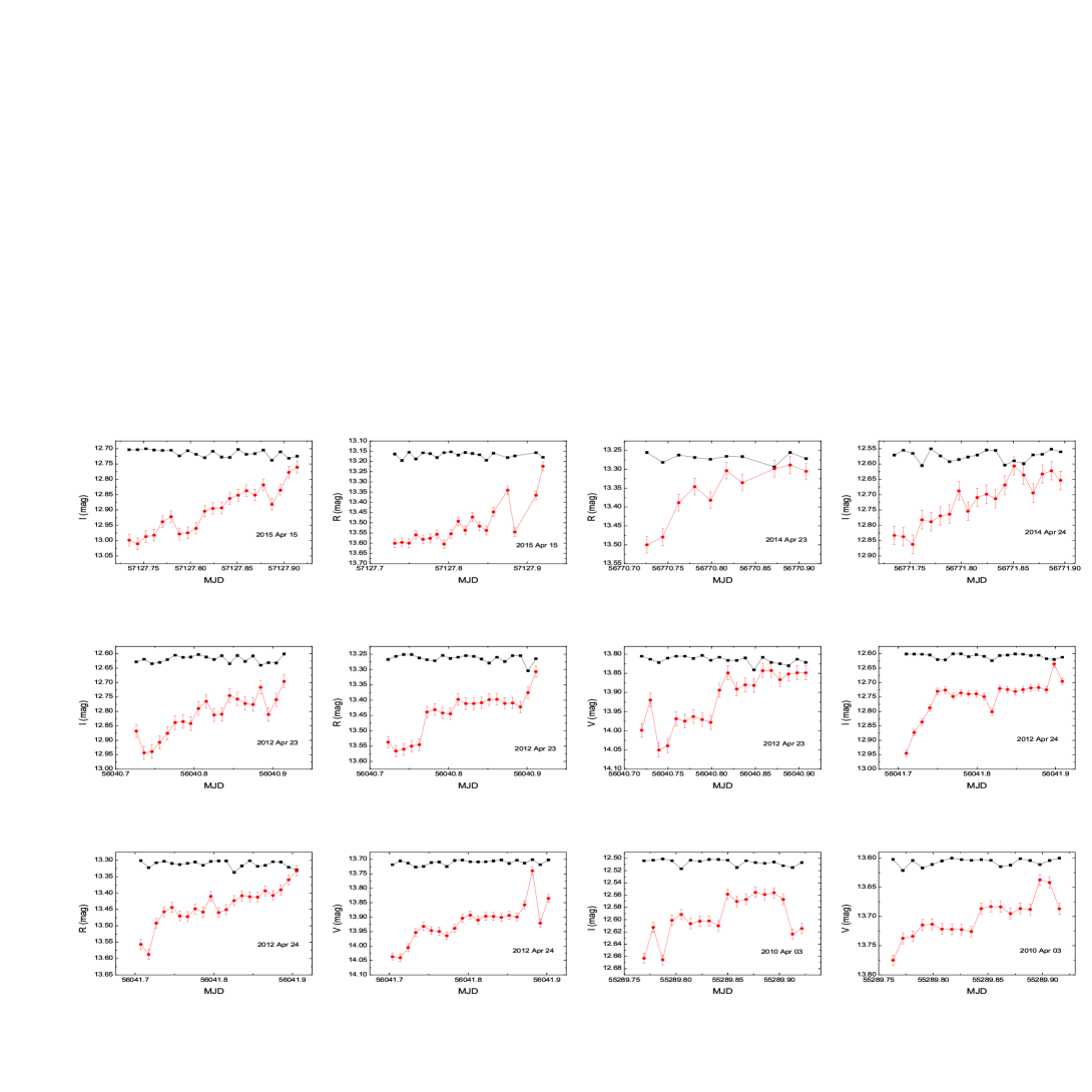
Figure 1: Light curves of intraday variability for Mrk 501. The red circles and lines are the light curves for Mrk 501. The black squares and lines are the variations of $S_{I}$, $S_{R}$ and $S_{V}$. The light curves of $S_{I}$, $S_{R}$ and $S_{V}$ are offset to avoid their eclipsing with light curves of Mrk 501.

where Var(BL-StarA), Var(BL-StarB) and Var(StarA-StarB) are the variances of differential instrumental magnitudes. The $F$ value from the average of $F_{1}$ and $F_{2}$ is compared with the critical $F$-value, $F^{\alpha}_{\nu_{bl},\nu_{\ast}}$, where $\nu_{bl}$ and $\nu_{\ast}$ are the number of degrees of freedom for the blazar and comparison star respectively ($\nu=N-1$), and $\alpha$ is the significance level set as 0.01 (2.6$\sigma$). If the average $F$ value is larger than the critical value, the blazar is variable at a confidence level of 99 per cent. de Diego (2010) presented that the ANOVA is powerful and robust estimator for microvariations. It does not rely on error measurement but derives the expected variance from subsamples of the data. The results of de Diego (2010) showed that according to the choice of one-minute exposures, a group of around five such exposures, lasting less than 10 minute accounting for CCD read-out, is a reasonable methodological choice for the ANOVA with 30 minute lags observational strategy. In order to obtain good S/N ratio, our exposure time were chose from 150 to 400 s. Considering the time interval of 10 minutes within each group (because 10 minutes is a safe time interval to bin data sharing similar flux characteristics), we bin the data in a group of three observations. This method is used only for light curves with more than 9 observations on a given night, but if the measurements in the last group are less than 3, then it is merged with the previous group. The critical value of ANOVA can be obtained by $F^{\alpha}_{\nu_{1},\nu_{2}}$ in the $F$-statistics, where $\nu_{1}=k-1$ ($k$ is the number of groups), $\nu_{2}=N-k$ ($N$ is the number of measurements) and $\alpha$ is the significance level (Hu et al. 2014). Our analysis results on intraday variability are shown in Table 5. The blazar is considered as variability only when the light curve satisfies the above three criteria. The blazar is considered as probably variable if one of the above three criteria is satisfied. The blazar is considered as non-variable if none of the criteria are met. From Table 5, it is seen that there is intraday variability found on 6 nights (2015 April 15, 2014 April 23, 2014 April 24, 2012 April 23, 2012 April 24, 2010 April 03). The corresponding light curves are seen in Fig. 1. In order to further quantify the reliability of variability, the $S_{x}$ is given in Fig. 1. The value of $S_{x}$ can be calculated as (e.g. Hu et al. 2014)

$$S_{x}=m_{i}-\overline{m},~{}~{}~{}x=V,R,I$$ (5)

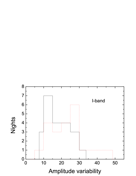
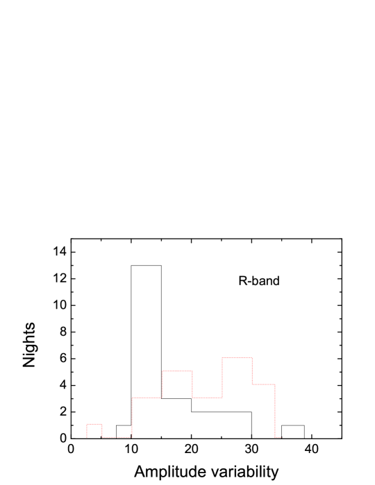
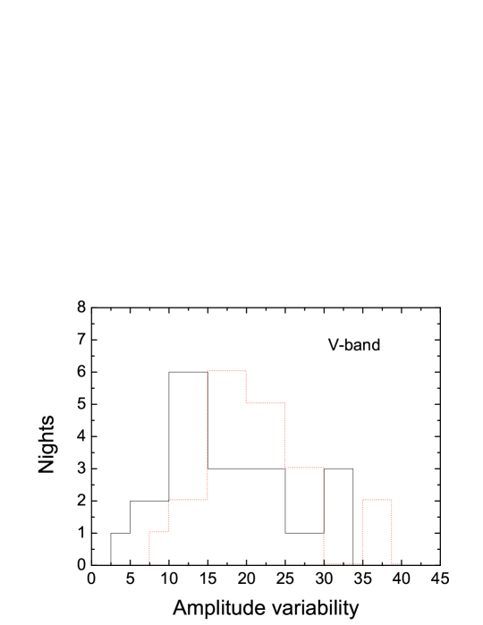
Figure 2: The intraday variability amplitude distribution in $I$, $R$ and $V$ bands. The black solid lines stand for non-correcting results and the red dotted lines for results of correcting Galactic extinction and the host galaxy contributions.

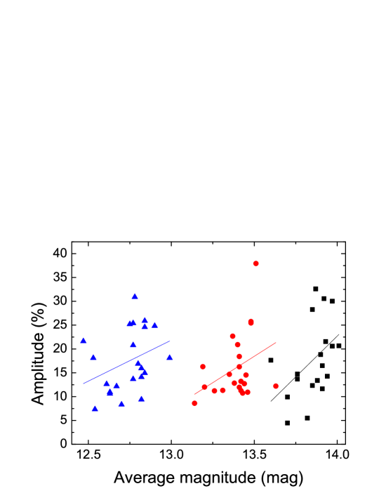
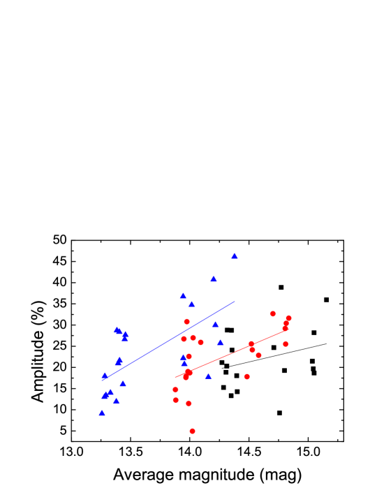
Figure 3: The variability amplitude versus the average brightness. The top panel is the results of non-correcting Galactic extinction and the host galaxy contributions, and the bottom panel is the correcting results. The blue triangles, red circles and black squares stand for $I$, $R$ and $V$ bands respectively. The lines are the best linear fitting for the three bands.

where $m_{i}$ and $\overline{m}$ are same with Equation (1). On 2015 April 15, the $I$ and $R$ bands show intraday variability, and the $V$ band is probably variable. For the night, the largest magnitude change of $I$ band is $\bigtriangleup I=0^{\rm m}.25$ in 246 minutes from MJD=57127.743 to MJD=57127.914. For the $R$ band on this night, Mrk 501 brightens by $\bigtriangleup R=0^{\rm m}.20$ in 39 minutes from the beginning of MJD=57127.848 to MJD=57127.875, and then quickly fades by $\bigtriangleup R=0^{\rm m}.21$ in 13 minutes from MJD=57127.875 to MJD=57127.884. The largest magnitude change of $R$ band is $\bigtriangleup R=0^{\rm m}.32$ in 52 minutes from MJD=57127.884 to MJD=57127.920. On 2014 April 23, the magnitude change of $R$ band is $\bigtriangleup R=0^{\rm m}.15$ in 79 minutes from MJD=56770.726 to MJD=56770.781. On 2014 April 24, the largest magnitude change of $I$ band is $\bigtriangleup I=0^{\rm m}.26$ in 141 minutes from MJD=56771.753 to MJD=56771.851. On 2012 April 23, the largest magnitude change of $I$ band is $\bigtriangleup I=0^{\rm m}.25$ in 256 minutes from MJD=56040.736 to MJD=56040.914, the magnitude change of $R$ band is $\bigtriangleup R=0^{\rm m}.11$ in 14 minutes from MJD=56040.763 to MJD=56040.773 and $V$ band $\bigtriangleup V=0^{\rm m}.13$ in 14 minutes from MJD=56040.730 to MJD=56040.740. On 2012 April 24, the magnitude change of $I$ band is $\bigtriangleup I=0^{\rm m}.22$ in 58 minutes from MJD=56041.710 to MJD=56041.750, $R$ band $\bigtriangleup R=0^{\rm m}.14$ in 43 minutes from MJD=56041.717 to MJD=56041.747 and $V$ band $\bigtriangleup V=0^{\rm m}.18$ in 14 minutes from MJD=56041.882 to MJD=56041.892. On 2010 April 03, the largest magnitude change of I band is $\bigtriangleup I=0^{\rm m}.11$ in 91 minutes from MJD=55289.787 to MJD=55289.850 and $V$ band $\bigtriangleup V=0^{\rm m}.14$ in 194 minutes from MJD=55289.763 to MJD=55289.898. The variability amplitude (Amp) for each night is given in Table 5 and Fig. 2. The distributions of variability amplitudes in $I$ and $V$ bands are from a few percent to $35\%$ ($R$ band extends to $40\%$), and most from $10\%$ to $15\%$. The relationships between variability amplitudes and the source average brightness (see Table 5) are shown in Fig. 3. The correlation between variability amplitudes and average brightness is found in the three bands (the coefficients of linear regression analysis $r_{\rm I}=0.33$, $r_{\rm R}=0.36$, $r_{\rm V}=0.45$), i.e. larger variability amplitude with a fainter brightness.

The duty cycle (DC) of Mrk 501 is calculated as (Romero et al. 1999; Stalin et al. 2009; Hu et ai. 2014)

$${\rm DC}=100\frac{\sum^{n}_{i=1}N_{i}(1/\triangle T_{i})}{\sum^{n}_{i=1}(1/\triangle T_{i})}{\rm per~{}cent},$$ (6)

where $\triangle T_{i}=\triangle T_{i,obs}(1+z)^{-1}$, $z$ is the redshift of the object and $\triangle T_{i,obs}$ is the duration of the monitoring session of the ith night. Note that since for a given source the monitoring durations on different nights were not always equal, the computation of DC has been weighted by the actual monitoring duration $\triangle t_{i}$ on the ith night. $N_{i}$ will be set to 1 if intraday variability is detected, otherwise $N_{i}=0$ (Goyal et al. 2013). When calculating the value of DC, we only consider nights with more than 9 points and monitoring longer than one hour. The value of DC is 16.65 per cent for Mrk 501 (54.13 per cent, if PV cases are also included).

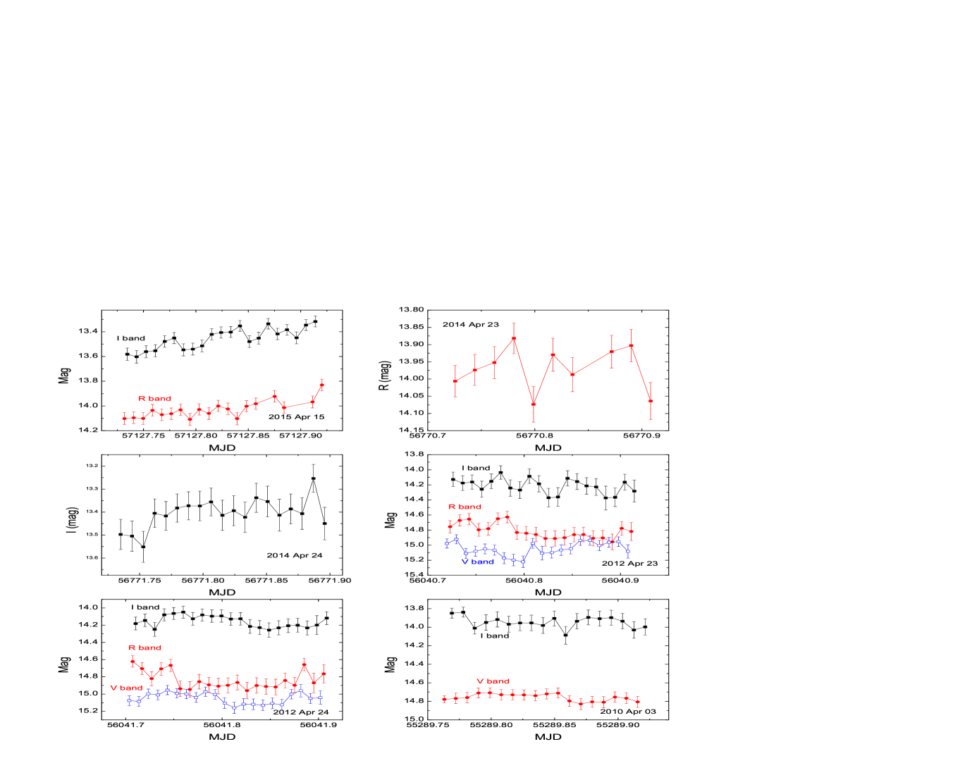
Figure 4: Light curves (corrected Galactic extinction and the host galaxy contributions) for Mrk 501. The black filled squares, red filled circles and blue empty squares are $I$, $R$ and $V$ bands respectively.

Galactic extinction is corrected with the coefficients ($A_{\rm I}=0^{\rm m}.029$, $A_{\rm R}=0^{\rm m}.041$, $A_{\rm V}=0^{\rm m}.052$) given in Schlafly & Finkbeiner (2011) who recalibrated the results of Schlegel et al. (1998). Following Gaur et al. (2015), Agarwal & Gupta (2015) and Aleksic et al. (2015), we subtract the host galaxy contributions from the observed fluxes in $R$ band by considering different aperture radii used by different observatories using the measurements of Nilsson et al. (2007). The host galaxy contributions in $I$ and $V$ bands are obtained by adopting the elliptical galaxy colors of $V-R=0.61$, $R-I=0.70$ from Fukugita et al. (1995). Then we subtract the host galaxy contributions from the observed fluxes in $I$ and $V$ bands. The magnitudes of $I$, $R$ and $V$ bands can be converted into fluxes (in mjy) using $F_{I}=2550\times 10^{-0.4\ast I}\times 10^{3}$, $F_{R}=3080\times 10^{-0.4\ast R}\times 10^{3}$ and $F_{V}=3640\times 10^{-0.4\ast V}\times 10^{3}$ respectively (Mead et al. 1990). The fluxes of host galaxy from different aperture radii used by different observatories are given in Table 2-4. We calculate the error of correcting magnitude (subtracted the host galaxy contributions) using error propagation from errors of observed magnitude and host galaxy magnitude. After correcting Galactic extinction and the host galaxy contributions, we only use ANOVA to reanalyze the intraday variability of the object. The blazar is considered as intraday variability when the light curve satisfies the ANOVA criterion. Then there are 10 nights detected as intraday variability ($I$ bands of 2015 April 06, 15, May 25, 2014 April 22, and 2012 April 24, $R$ bands of 2015 April 08, 15, 2012 April 23-24 and 2010 April 01, $V$ bands of 2015 May 25, 2014 April 23, 2012 April 23 and 2010 April 03). These nights ($I$ and $V$ of 2015 May 25, $I$ band of 2014 April 22 and $V$ band of 2014 April 23) are though as PV from results of non-correcting host galaxy contributions because the light curves satisfy the ANOVA criterion but dissatisfy $C$ and/or $F$ tests criteria. The three nights ($I$ band of 2015 April 06, $R$ bands of 2015 April 08 and 2010 April 01) are not considered as intraday variability from non-correcting results. These nights ($I$ bands of 2014 April 24, 2012 April 23 and 2010 April 03, $R$ band of 2012 April 24, $V$ band of 2012 April 24) are detected as intraday variability from non-correcting results, but not as intraday variability from correcting results. In order to compare with Fig. 1, a fraction of the light curves (corrected Galactic extinction and the host galaxy contributions) are given in Fig. 4. The results of magnitude change are given in Table 6. From Table 6, it is seen that the results of magnitude change for correcting and non-correcting Galactic extinction and the host galaxy contributions are different, and the variability status of partial nights has changed. We take a variability to be real if the variability is three times greater than $\sigma$ (Fan et al. 2014). For the non-correcting results, the largest magnitude change is $\bigtriangleup R=0^{\rm m}.32$ in 52 minutes and the shortest timescale is 13 minutes with $\bigtriangleup R=0^{\rm m}.21$. For the correcting results, we obtain that the largest magnitude change is $\bigtriangleup R=0^{\rm m}.31$ in 72 minutes. The correcting variability amplitude (Amp) for each night is also given in Fig. 2. The Fig. 2 shows that the average variability amplitude of correcting magnitude ($<{\rm Amp}>_{I}=23.82\%,<{\rm Amp}>_{R}=22.25\%,<{\rm Amp}>_{V}=22.05\%$) is larger than that of non-correcting magnitude. There are still correlations between variability amplitude (Amp) and average brightness from correcting results ($r_{I}=0.67,r_{R}=0.59,r_{V}=0.29$; see Fig. 3). The correcting value of DC is 14.87 per cent excluding these nights ($I$ and $V$ of 2015 May 25, $I$ band of 2014 April 22 and $V$ band of 2014 April 23), since when calculating the DC of non-correcting magnitude, these nights are not considered in spite of meeting ANOVA criterion.

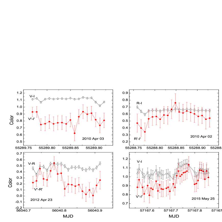
Figure 6: Color indices variations with time for intraday timescale. The black empty circles stands for color indices of non-correcting host galaxy contributions, and red filled circles for color indices of correcting host galaxy contributions.

Long-term light curves and color indices variations of our observations are shown in Fig. 5. From Fig. 5, it is seen that for correcting and non-correcting results, the source shows variability and color indices variability on short timescale and long timescale in the three bands. The overall magnitude changes and color indices variability are $\bigtriangleup I=0^{\rm m}.75$, $\bigtriangleup R=0^{\rm m}.62$, $\bigtriangleup V=0^{\rm m}.64$, $\bigtriangleup(V-R)=0^{\rm m}.4$, $\bigtriangleup(V-I)=0^{\rm m}.47$ and $\bigtriangleup(R-I)=0^{\rm m}.43$ for non-correcting results, and $\bigtriangleup I^{\prime}=1^{\rm m}.53$, $\bigtriangleup R^{\prime}=1^{\rm m}.33$, $\bigtriangleup V^{\prime}=1^{\rm m}.21$ $\bigtriangleup(V^{\prime}-R^{\prime})=0^{\rm m}.7$, $\bigtriangleup(V^{\prime}-I^{\prime})=0^{\rm m}.76$ and $\bigtriangleup(R^{\prime}-I^{\prime})=0^{\rm m}.77$ for correcting results. We also use all three variability tests to quantify the variability of color indices ($V-R$, $V-I$ and $R-I$). On 2010 April 03, the color indices $V-I$ is detected as variability for non-correcting results, but the rest of nights are not detected as variability for non-correcting results. After correcting the host galaxy contributions, there are three nights detected as variability ($V-I$ on 2015 May 25, $V-R$ on 2012 April 23 and $R-I$ on 2010 April 02). The corresponding color indices variations with time are seen in Fig. 6. On 2012 April 23, the source shows IDV in $VR$ bands. The result supports that flux variations are associated with the color variations on intraday timescale.

3.2 Cross-correlation analysis and variability timescale

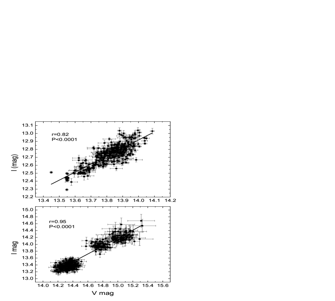
Figure 7: The $I$ band magnitude versus $V$ band magnitude for non-correcting (top panel) and correcting (bottom panel) host galaxy contributions. The solid lines are the results of linear regression analysis. $r$ is the correlation coefficient; $P$ is the chance probability.

We perform the inter-band correlation analysis and searched for the possible inter-band time delay. First, the $V$ band magnitude versus $I$ band magnitude is given in Fig. 7. The Fig. 7 and linear regression analysis show that there are strong correlations between the $V$ band magnitude and $I$ band magnitude. The interpolated cross-correlation function (ICCF; Gaskell & Peterson 1987) and the discrete correlation function (DCF; Edelson & Krolik 1988) are standard techniques in time series analysis for finding time lags between light curves at different wavelengths. Apart from the ICCF and DCF, there is another method of estimating the cross-correlation function (CCF) in the case of non-uniformly sampled light curves, the z-transformed discrete correlation function (ZDCF; Alexander 1997). It has been shown in practice that the calculation of the ZDCF is more robust than that of the ICCF and the DCF when applied to sparsely and unequally sampled light curves (e.g., Edelson et al. 1996; Giveon et al. 1999; Roy et al. 2000). The ZDCF is used in our analysis. The ZDCF code of Alexander (1997) can automatically set how many bins are given and used to calculate the inter-band correlation on intraday and long time scales. In order to keep the validity of the statistical data, we set minimal ten number of points per bin. For magnitude of non-corrected host galaxy contributions, the part of the results are displayed in Fig. 8. For each correlation, a Gaussian fitting is made to find the central ZDCF points. The time where the Gaussian profile peaks denotes the lag between the correlated light curves (Wu et al. 2012). From Fig. 8 and results of Gaussian fitting, and considering time resolutions and spans, we can find that there are not significant time lags between the $V$ band magnitude and $I$ band magnitude. For some nights and long time scales, we have not enough data points to find time lags because most of nights have less than 20 data points and there is large observed time interval for long time scale. The correcting results from ZDCF analysis are consistent with non-correcting results.

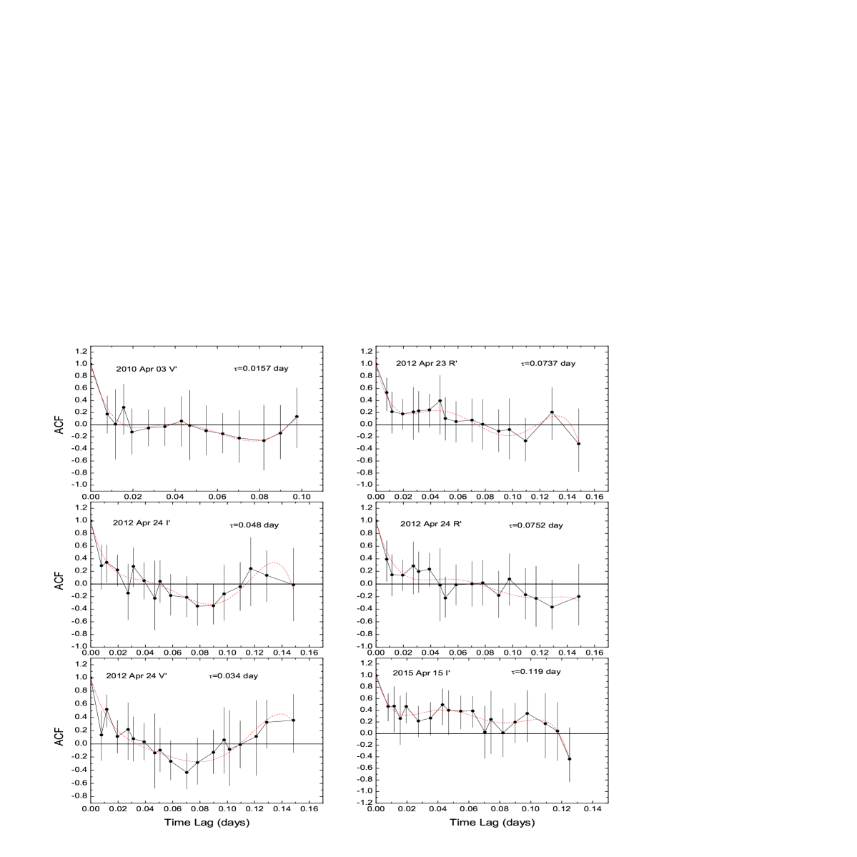
Figure 9: The ACF analysis for results of correcting the host galaxy contributions. The red dash line is a fifth-order polynomial least-squares fit.

The zero-crossing time of the autocorrelation function (ACF) is a well-defined quantity and is used as a characteristic variability timescale (e.g. Alexander 1997; Giveon et al. 1999; Netzer et al. 1996; Liu et al. 2008). If there is an underlying signal in the light curve, with a typical timescale, then the width of the ACF peak near zero time lag will be proportional to this timescale (Giveon et al. 1999; Liu et al. 2008). Following Giveon et al. (1999) and Liu et al. (2008), we choose the zero-crossing time of the ACF as the variability timescale. In addition, the first-order structure function (SF; Trevese et al. 1994) can also be used to analyze a characteristic variability timescale. There is a simple relation between the ACF and the SF (see equation (8) in Giveon et al. 1999). In this paper, only an ACF analysis is performed to search for the presence of any characteristic variability timescale. We estimate the ACF also using the ZDCF code from Alexander (1997), and only analyze the nights detected as intraday variability. After correcting the host galaxy contributions, the results used to estimate characteristic variability timescale are given in Fig. 9. We then used a least-squares procedure to fit a fifth-order polynomial to the ZDCF, with the constraint that ACF($\tau$=0)=1 (Giveon et al. 1999). From Fig. 9 and fitting results, intraday variation timescales of $\sim 23$ to $\sim 171$ minutes were detected. The most common definition of the variability timescale $\tau=F/(|\triangle F/\triangle t|)$ has the advantage of weighting fluctuations by their amplitudes, where $F$ is the flux density at the minimum, and $\triangle F$ is the variability amplitude in the timescale $\triangle t$ (e.g. Wagner & Witzel 1995; Liu et al. 2008). The variation timescale is defined as variations of $\triangle F/F\geq 30\%$ between the subsequent minimum and maximum within the timescale $\triangle t$, and $\triangle F>3\sigma$ (Liu et al. 2008; Fan et al. 2014). In order to further confirm reliability of the variation timescales, we check the corresponding light curves, and find that 2012 April 23 $R^{\prime}$ (from 56040.783 to 56040.822), 2012 April 24 $R^{\prime}$ (from 56041.757 to 56041.707) and 2015 April 15 $I^{\prime}$ (from 57127.743 to 57127.915) satisfy the criteria of the variation timescales (see Fig. 4). Therefore, from our results, three characteristic timescales 0.0737 0.0752, and 0.119 days are detected. Among them, the 0.0737 day $\sim$106 min from 2012 April 23 is the minimal characteristic variability timescale.

3.3 Correlation between Magnitude and Color Index

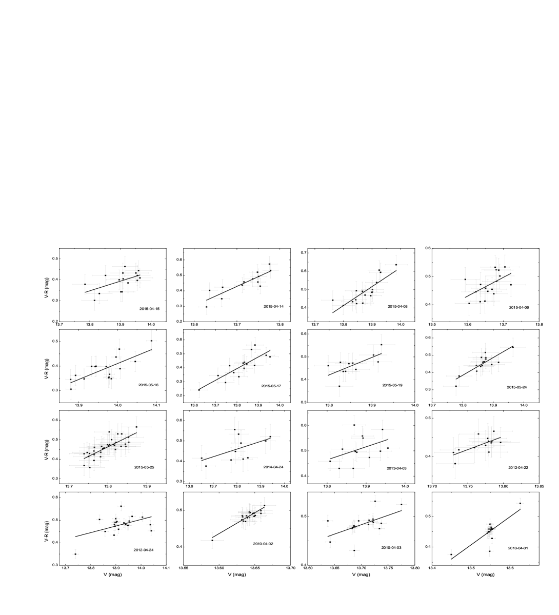
Figure 10: The correlations between $V-R$ index and $V$ magnitude for non-correcting the host galaxy contributions. The solid lines is results of linear regression analysis.

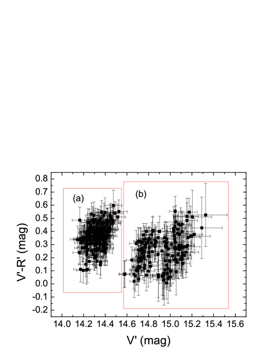
Figure 11: The correlations between $V-R$ index and $V$ magnitude for long-term timescale. The top panel is the results of non-correcting the host galaxy contributions, and the bottom panel is the correcting results.

In order to explore the optical spectral properties, we analyze the correlation between magnitude and color index for intraday, short-term, and long-term timescales. The relation between $V-R$ index and $V$ magnitude is frequently studied, so we concentrate on $V-R$ index and $V$ magnitude. When exploring the correlation for intraday timescale, we only analyze the nights with the number of $V-R$ index $N\geq 9$. For the color index, first, we correct the Galactic extinction. After correcting the Galactic extinction, the results of correlations between $V-R$ index and $V$ magnitude are given in Table 7. Then the results of correcting the host galaxy contributions are also given in Table 7. As an example, Fig. 10 shows the correlations between $V-R$ index and $V$ magnitude for non-correcting the host galaxy contributions on intraday timescale. From Fig. 10 and Table 7, it is seen that most of nights have strong correlations between $V-R$ index and $V$ magnitude on intraday timescale for non-correcting and correcting the host galaxy contributions. There are three nights with moderate correlations for correcting or non-correcting the host galaxy contributions (2010 April 01, 2012 April 24 and 2013 April 03). So a bluer-when-brighter (BWB) chromatic trend is dominant for Mrk 501 on intraday timescale. And the BWB trend exists in active and stable state because in our observations, some nights show IDV, while others do not. There is still a strong BWB trend on short-term timescale (2010 April 01-03, 2012 Apr 22-24 and 2013 Apr 01-04 from Table 7). In a intermediate-term timescale (weeks to months), the correlations weaken (see Table 7). For long-term timescale, the correlations for correcting the host galaxy contributions are stronger than that for non-correcting the host galaxy contributions (2014 Apr 19-May 08 and 2015 Apr 06-May 25 from Table 7). The correlations between $V-R$ index and $V$ magnitude in long-term timescales are shown in Fig. 11. The analysis of spearman rank obtains that there is a weak correlations between $V-R$ index and $V$ magnitude for non-correcting the host galaxy contributions ($r=0.1,P=0.06$). For all data subtracted the host galaxy contributions, there is significant negative correlation between $V-R$ index and $V$ magnitude ($r=-0.235,P=1\times 10^{-5}$), i.e. redder-when-brighter (RWB). However, if we inspect the Fig. 11 in detail, we can find two separate regions (a) and (b). The dividing line is $V\sim 14^{\rm m}.55$. For region (a), there is significant correlation with $V-R\sim 0.48(\pm 0.08)V$ ($r=0.38,P=1\times 10^{-6}$) and significant correlation with $V-R\sim 0.29(\pm 0.06)V$ ($r=0.35,P=9\times 10^{-6}$) for region (b). The correlation coefficient and slope of region (a) are larger than that of region (b), i.e. compared with low flux state, the BWB behavior is more pronounced at high flux state.

4 DISCUSSION AND CONCLUSIONS

Most blazars show microvariability/IDV in a few hours/minutes, but the unpredictability of these changes in brightness and the difficulty of obtaining confirmation by others have been an incredible cause (de Diego 2010). Generally, $C$ test is used for quantifying the IDV. de Diego (2010) presented that $C$ test is not a reliable methodology, and that $F$ test and ANOVA are powerful and robust estimators for IDV. In order to increase the confidence on the validity of IDV, the blazar is considered as IDV only when the light curve satisfies all the three criteria. For ANOVA, The results of de Diego (2010) showed that a binning of five observations is a reasonable methodological choice for the ANOVA with 30 minute lags observational strategy. But considering our exposure time, we bin the data in a group of three observations. Note that the smallest bin sizes improve the time resolutions, but the detections are biased toward large amplitude (de Diego 2010). The CCD aperture photometry obtains the optical magnitude by comparing the object brightness to the brightness of several comparison stars in the field of the object which causes that changes in sky transparency can be eliminated and accuracies $<1\%$ attained even under varying conditions (Nilsson et al. 2007). However, the presence of a strong host galaxy component can affect measured aperture photometry. Mrk 501 has strong host galaxy components. If the host galaxy contribution are not subtracted, the broadband spectra are highly distorted and relative optical flux variations underestimated. FWHM changes do not introduce very strong false variability in objects with a prominent host galaxy component (0.01-0.03 mag; Cellone et al. 2000; Nilsson et al. 2007). For our observations, The aperture radius of 2$\times$FWHM or 1.5$\times$FWHM was selected, and the scale of aperture radius is same on the same night. The value of FWHM is associated with seeing. One night, the value of FWHM almost is constant, but the small seeing change can still cause changes of FWHM and aperture radius. These can bring in false variability in objects with a prominent host galaxy component. For a longer-term timescale, different nights or periods are likely to have larger seeing change which may cause larger false variability in objects with a prominent host galaxy component. Therefore, for the objects with a prominent host galaxy component, the correcting host galaxy components are needed. We subtract the host galaxy contributions from the observed fluxes in $R$ band by considering different aperture radii used by different observatories using the measurements of Nilsson et al. (2007). The host galaxy contributions in $I$ and $V$ bands are not obtained from direct measurements but from conversion of colors. This may introduce uncertainty.

Long-term quasi-simultaneous multi-band observations of blazar Mrk 501 were performed from 2010 to 2015 in $V$, $R$ and $I$ bands. Our monitoring program for Mrk 501 was divided into five different periods. In total, we observed 29 nights and 1186 CCD frames with error less than 0.05 mags. For our results of non-correcting host galaxy contributions, the magnitude distributions in $V$, $R$ and $I$ bands are $14^{\rm m}.14<V<13^{\rm m}.50$, $13^{\rm m}.71<R<13^{\rm m}.08$ and $13^{\rm m}.07<I<12^{\rm m}.32$, and mean values $<V>=13^{\rm m}.85\pm 0^{\rm m}.12$, $<R>=13^{\rm m}.38\pm 0^{\rm m}.12$ and $<I>=12^{\rm m}.74\pm 0^{\rm m}.14$. The magnitude distributions in $VRI$ bands in 1995-1996 from Xie et al. (1999) are $14^{\rm m}.16-13^{\rm m}.79$, $13^{\rm m}.72-13^{\rm m}.20$ and $13^{\rm m}.17-12^{\rm m}.62$ respectively. The magnitude distribution in $R$ band in 1999 from Xie et al. (2001) is from $13^{\rm m}.04$ to $12^{\rm m}.96$. The magnitude distribution in $R$ band in 2000 from Dai et al. (2001) is from $13^{\rm m}.77$ to $13^{\rm m}.09$. The magnitude distributions in $VR$ bands in 2000 from Gupta et al. (2008) are $13^{\rm m}.77-13^{\rm m}.59$ and $13^{\rm m}.45-13^{\rm m}.17$ respectively. The magnitude distribution in $R$ band in 2007-2012 from Wierzcholska et al. (2015) is from $13^{\rm m}.57$ to $13^{\rm m}.37$. The magnitude distribution in $V$ band in 2011-2012 from Shukla et al. (2015) is from $14^{\rm m}.05$ to $13^{\rm m}.87$. From above references and NASA/IPAC Extragalactic Database: NED, we obtain that the maximum and minimum magnitude for this source till data are $14^{\rm m}.16-13^{\rm m}.39$ (Xie et al. 1999; Hutter & Mufson 1981), $13^{\rm m}.77-12^{\rm m}.64$ (Dai et al. 2001; Hutter & Mufson 1981) and $13^{\rm m}.17-12^{\rm m}.21$ (Xie et al. 1999; Sitko et al. 1983) for $V$, $R$ and $I$ bands respectively. Through comparisons, it is seen that our distributive ranges of magnitude in $VRI$ bands are basically consistent with others.

4.1 Variability

Optical photometric observations of blazars are important tools for constructing their light curves which can yield valuable information about the mechanisms operating in these sources, with important implications for blazars modeling (e.g. Fan et al. 2009). Variability timescale is one of the observational characteristics of blazars. Detailed knowledge of the statistical behaviors on different timescales is therefore very useful to understand the basic physical mechanisms during the flaring and quiescent phases (Dai et al. 2015; Ciprini et al. 2003).

From our analysis, for results of non-correcting host galaxy contributions, there is intraday variability found on 6 nights. The distributions of variability amplitudes in $I$ and $V$ bands are from a few percent to $35\%$ ($R$ band extends to $40\%$), and most from $10\%$ to $15\%$. The value of DC is 16.65 per cent for Mrk 501 (54.13 per cent, if PV cases are also included). Goyal et al. (2013) found that for TeV blazars the DC is $45\%$ and if IDV with variability amplitudes ${\rm Amp}>3\%$ is considered, the DC is $32\%$. Our average variability amplitude is much larger than that of TeV blazars from table 1 of Goyal et al. (2013). So compared with other TeV blazars, the Mrk 501 may have large variability amplitude and low DC. Making use of results of Nilsson et al. (2007), we subtract the host galaxy contributions from the observed fluxes. The correcting results show that the results of magnitude change for correcting and non-correcting the host galaxy contributions are different, and the variability status of partial nights has changed. These are mainly because the seeing change causes changes of FWHM and aperture radius. After correcting the host galaxy contributions, the variability status and magnitude variabilities will change. The average variability amplitude of correcting magnitude is larger than that of non-correcting magnitude, which supports that the relative optical flux variations are underestimated for results of non-correcting host galaxy contribution. If the optical flux variations include object and host galaxy components, and host galaxy is more likely to be as stable component, after subtracting host galaxy component, the variability amplitude will increase. The correcting value of DC is slightly smaller than the non-correcting value. The results of Xie et al. (1996) showed that intraday variability amplitude of Mrk 501 is smaller than 0.22 mag in the $B$ and $V$ bands. From results of Xie (1999, 2001), Dai et al. (2001), Gupta et al. (2008), Wierzcholska et al. (2015) and Shukla et al. (2015), for Mrk 501, the intraday variability amplitude with more than 0.3 mag is rare. Long-term light curves of our observations show that the overall magnitude changes are $\bigtriangleup I=0^{\rm m}.75$, $\bigtriangleup R=0^{\rm m}.62$ and $\bigtriangleup V=0^{\rm m}.64$ for non-correcting results, and $\bigtriangleup I=1^{\rm m}.53$, $\bigtriangleup R=1^{\rm m}.33$ and $\bigtriangleup V=1^{\rm m}.21$ for correcting results. Xie et al. (1999) presented that Mrk 501 show the largest variation $\triangle V=0^{\rm m}$.8 during 345 days. From Xie (1999, 2001), Dai et al. (2001), Gupta et al. (2008), Wierzcholska et al. (2015) and Shukla et al. (2015), the variability amplitude in long-term timescale from $0^{\rm m}.2$ to $0^{\rm m}.7$ are observed. From results of ACF and analysis of light curves, a minimal variability timescale of $\sim 106$ min in $\triangle R^{\prime}=0.31$ is detected. Ghosh et al (2000) found that the observed variability of Mrk 501 by 0.13 mag within 12 minutes. Xie et al. (1999) presented that the Mrk 501 has a flare of $\Delta R=0.49$ in 105 minutes. Gupta et al. (2008) found that the Mrk 501 has a flare of $\Delta R\sim 0.05$ in 15 minutes. So our minimal variability timescale is consistent with result from Xie et al. (1999). If the observed minimum timescale indicates an innermost stable orbital period, an upper limit can be obtained for the mass of the central black hole (e.g. Xie et al. 2004; Fan et al. 2014; Dai et al. 2015). From Fan (2005) and Fan et al. (2014), the innermost stable orbit depends on the black hole and the accretion disk, and $r\leq c\delta\triangle t_{\rm min}/(1+z)$, and then the upper limits of black hole masses are (i) $M_{8}\leq 1.2\times\frac{\delta\triangle t_{\rm min}(hr)}{1+z}$ for a thin accretion disk surrounding a Schwarzschild black hole; (ii) $M_{8}\leq 1.8\times\frac{\delta\triangle t_{\rm min}(hr)}{1+z}$ for a thick accretion disk surrounding a Schwarzschild black hole; (iii) $M_{8}\leq(\frac{7.3}{1+\sqrt{1-a^{2}}})(\frac{\delta\triangle t_{\rm min}(hr)}{1+z})$ for the case of a Kerr black hole, where $M_{8}$ is the black hole mass in units of $10^{8}M_{\odot}$, and $a$ is an angular momentum parameter. Then we obtain the upper limits of black hole mass are $M\leq 10^{8.99}M_{\odot}$ and $M\leq 10^{9.17}M_{\odot}$ for a thin and thick accretion disks, and $M\leq 10^{9.78}M_{\odot}$ for the extreme Kerr black hole case ($a=1$) with Doppler factor 4.8 from Wu et al. (2007). Considering the minimal variability timescale as the light crossing time of the emitting volume (e.g. Dai et al. 2015), the size of the emitting region $r\leq 8.9\times 10^{14}$ cm is also estimated. Woo & Urry (2002) and Sbarrato et al. (2012) estimated virial black hole mass for AGNs. The black hole masses of Mrk 501 from Woo & Urry (2002) and Sbarrato et al. (2012) are $10^{9}M_{\odot}$ and $10^{9.21}M_{\odot}$ respectively. Therefore, our upper limits of black hole mass estimated from variability timescale is consistent with results of Woo & Urry (2002) and Sbarrato et al. (2012).

In order to explain the optical IDV, many intrinsic and extrinsic models have been proposed. The intrinsic models include shock-in-jet model (Marscher & Gear 1985; Marscher et al. 2008) and accretion disc model (Chakrabarti & Wiita 1993; Mangalam & Wiita 1993). Extrinsic mechanisms involve interstellar scintillation and geometrical effects (Heeschen et al. 1987; Gopal-Krishna & Wiita 1992). The interstellar scintillation leads to radio variations at low frequencies and can therefore not be the case of optical intraday variability (Agarwal & Gupta 2015). The long-term periodic and achromatic BL Lacertae variability may be mostly explained by the geometrical scenarios where viewing angle variation can be due to the rotation of an inhomogeneous helical jet which causes variable Doppler boosting of the corresponding radiation (e.g. Gaur et al. 2015; Larionov et al. 2010, Villata et al. 2002). Among the several accepted theoretical models explaining variability, for Mrk 501 in high state, the origin of IDV and STV can be attributed to the shock-in-jet model. The accretion disc models are not likely to explain the IDV because the accretion disk radiation is always overwhelmed by the Doppler boosting flux from the relativistic jet, and Mrk 501 has a radiatively inefficient accretion discs (Urry & Padovani 1995; Ghisellini et al. 2011; Sbarrato et al. 2012; Xiong et al. 2014). However, the blazars in low state, the origin of IDV can be explain by instability in the accretion disk, because in the low state, jet emission is less dominant over the emission from the disk. A weak emission from base of jet is an alternative way to explain the IDV of Mrk 501 in the low state (Gupta et al. 2008). Moreover, for high SMBH masses, the ligh crossing time is very large which can cause the variability of shortest timescale (Agarwal & Gupta 2015). On basis of the synchrotron self-Compton (SSC) mechanism, Shukla et al. (2015) presented that the observed optical and X-ray variability of Mrk 501 may be explained by the injection of fresh electrons in emission zones and cooling of the electrons.

For Mrk 501, one of the most fascinating features is the observed possible periodicity of $\sim$ 23 days in the TeV and X-ray band (e.g. Hayashida et al. 1998; kranich et al. 1999). Rieger & Mannheim (2000) presented that this periodicity possibly be related to the orbital motion of the relativistic jet in a binary black hole systems where the nonthermal radiation is emitted by a relativistic jet which emerges from the less massive black hole, the periodicity thus being due mainly to geometrical origin (i.e. Doppler-shifted modulation). The origin of the periodicity of $\sim$ 23 days may be explained by the instabilities of (optically thin) accretion disks (Fan et al. 2008). From our observations, we can not obtain possible periodic variability timescales for STV and LTV because there are not enough observed data points.

4.2 Relation of Color and Magnitude

For Mrk 501, the host galaxy contributions and Galactic extinction can lead to a unreal color variations. From our results, the BWB trend is dominant for Mrk 501 on intermediate, short and intraday timescales for both non-correcting and correcting host galaxy contributions. Compared with short timescale, the long timescale has a weaker BWB trend, and there is a weak BWB trend in the long timescale for non-correcting results. The long timescale are likely to have larger seeing change which may cause larger false variability in Mrk 501. So the weak BWB trend may be due to the contamination of host galaxy. In the case of non-correcting host galaxy contributions, Wierzcholska et al. (2015) and Ikejiri et al. (2011) have found significant overall BWB trend in long timescale for Mrk 501. We should note that the largest variability amplitudes of Mrk 501 from them are less than $0^{\rm m}.2$. Zheng et al. (2008) found that flux variations are associated with the color variations in long term timescale. Then the color variations may be related with active state of the object. For the results of them, it may stand for relatively quiet state. From our results, after correcting the host galaxy contributions, there is a overall RWB trend in the long timescale. It is possible that the RWB trend is due to superposition of different components (jet components, accretion disk components, Gravitational microlensing effect; Bonning et al. 2012; Fan et al. 2008; Gaur et al. 2015; Agarwal & Gupta 2015). The uncertainties of correcting host galaxy components may also cause the RWB trend. However, we can find two separate regions in the long-term timescale. The dividing line is $V\sim 14^{\rm m}.55$. The two separate regions show the BWB trend but have different slope of BWB. Therefore, for long-term timescale, Mrk 501 in different state can have different BWB trend, and compared with low flux state, the BWB behavior is more pronounced at high flux state.

The BWB trends is very well known for BL Lacs. It is important to recall that the underlying host galaxy, effect of the accretion disc component and the Gravitational microlensing can also lead to apparent, but unreal, color variations (Gaur et al. 2015; Hawkins 2002). Since Mrk 501 has a radiatively inefficient accretion discs; our results exclude the host galaxy contributions; Gravitational microlensing is important on weeks to months timescales, the source is a good candidate for studying color variations for intraday timescale. The BWB trend indicates “harder when brighter” behavior which is consistent with the shock-in-jet model (e.g. Dai et al. 2015). According to the shock-in-jet model, as the shock propagating down the jet strikes a region of high electron population, radiations at different visible colors is produced at different distances behind the shocks. High-energy photons from synchrotron mechanism typically emerge sooner and closer to the shock front than the lower frequency radiation thus causing color variations (Agarwal & Gupta 2015). From our results, the BWB trends on intermediate, short and intraday timescales support the shock-in-jet model. For long-term timescale, host galaxy effect, Doppler factor variation (Villata et al. 2004; Hu et al. 2014) and superposition of different components (Bonning et al. 2012; Gaur et al. 2015) may cause the weak BWB (non-corrected host galaxy contributions) or RWB trends (corrected host galaxy contributions). Moreover, for long-term timescale, the different states with different BWB trends support the result from Anderhub et al. (2009) and Acciari et al. (2011) that compared with low-activity state, the “harder when brighter” behavior are more pronounced at high-activity level. Finally, we should note that for color variations, simultaneous multi-band observations are needed.

The results of ZDCF analysis indicate that there are not significant time lags between the $V$ band magnitude and $I$ band magnitude. Generally, on short timescales, it is difficult to detect the time lags between two optical bands due to the closeness of the various optical bands (Gaur et al. 2015). We also found the smaller variability amplitude with a larger brightness which can be explained as the source flux increases, the irregularities in the turbulent jet decrease and the jet flow becomes more uniform leading to a decrease in amplitude of variability (Marscher 2014; Gaur et al. 2015).

5 SUMMARY

We have monitored the BL Lac object Mrk 501 in five periods from 2010 to 2015. The quasi-simultaneous multi-band observations in $VRI$ bands provide 1186 data points with error less than 0.05 mags. Our main results are the following:

(i) For results of non-correcting host galaxy contributions, there is intraday variability found on 6 nights. The distributions of variability amplitudes in $I$ and $V$ bands are from a few percent to $35\%$ ($R$ band extends to $40\%$), and most from $10\%$ to $15\%$. The value of DC is 16.65 per cent for Mrk 501 (54.13 per cent, if PV cases are also included). Long-term light curves of our observations show that the overall magnitude changes are $\bigtriangleup I=0^{\rm m}.75$, $\bigtriangleup R=0^{\rm m}.62$ and $\bigtriangleup V=0^{\rm m}.64$.

(ii) Compared with non-correcting results, after correcting host galaxy contributions, the magnitude change are different, and the IDV status of partial nights has changed. The average variability amplitude of correcting magnitude are larger than that of non-correcting magnitude. The correcting value of DC is slightly smaller than the non-correcting value. The overall magnitude changes are $\bigtriangleup I=1^{\rm m}.53$, $\bigtriangleup R=1^{\rm m}.33$ and $\bigtriangleup V=1^{\rm m}.21$.

(iii) There are inverse correlations between the variability amplitude and the average brightness both for non-correcting and correcting results. No significant time lag between $V$ and $I$ bands is found on one night. A minimal variability timescale of 106 minutes is detected.

(iv) The source shows color indices variability on intraday timescale, short timescale and long timescale. The flux variations are associated with the color variations on intraday timescale.

(v) The BWB trend is dominant for Mrk 501 on intermediate, short and intraday timescales for both non-correcting and correcting host galaxy contributions which supports the shock-in-jet model. For the long timescale, Mrk 501 in different state can have different BWB trend.

Figure 5: Long-term light curves of Mrk 501 in $I$, $R$, $V$ bands and color indices $V-R$, $V-I$ and $R-I$. The first and third rows of panels are the results of non-correcting host galaxy contributions, and the second and forth rows of panels are the results of correcting host galaxy contributions

Figure 8: The ZDCF plots between $V$ and $I$ bands. The curves show Gaussian fittings to the points, and their peaks are marked with the vertical lines. The corresponding time lags are $0.011\pm 0.007,-0.012\pm 0.003,-0.016\pm 0.005,-0.016\pm 0.011,-0.019\pm 0.012$ and $0.0016\pm 0.01$ in days for 2012 April 23, 2012 April 24, 2010 April 01-03, 2012 April 22-24, 2014 April 19-24 and 2015 May 16-25.

Table 1: Observation log of photometric observations

Date(UT)	Number(I,R,V)	Time spans(h)	Time resolutions(min)
2010 04 01	17,17,17	3.1	12
2010 04 02	20,20,20	4.1	13
2010 04 03	18,18,18	3.7	13
2012 04 22	18,18,15	4.3	14
2012 04 23	20,20,20	4.5	14
2012 04 24	21,21,21	4.8	14
2012 04 25	3,0,2	0.6	19
2013 04 01	10,9,9	2.8	17
2013 04 03	15,15,13	3.9	16
2013 04 04	5,6,5	1	14
2014 04 17	0,21,0	2	5
2014 04 19	11,8,7	3.6	20
2014 04 20	8,9,6	3.5	25
2014 04 22	11,10,9	4.4	25
2014 04 23	9,10,9	4.4	25
2014 04 24	19,16,12	3.9	13
2014 04 25	5,5,0	2.5	25
2015 04 06	15,18,17	3.2	14
2015 04 07	8,3,0	2.1	13
2015 04 08	19,18,18	3.9	13
2015 04 13	16,13,9	3.9	13
2015 04 14	14,14,17	3.6	13
2015 04 15	21,19,21	4.5	13
2015 05 16	20,19,20	3.4	9
2015 05 17	18,17,15	3.3	10
2015 05 19	11,12,11	3.4	12
2015 05 24	28,22,24	6.8	10
2015 05 25	44,38,39	8	10

Table 2: Data of $I$ Band

Date(UT)	MJD	Magnitude	$\sigma$	$F_{host}$(mJy)
2010 Apr 01	55287.782	12.539	0.015	11.1
2010 Apr 01	55287.790	12.521	0.015	12
2010 Apr 01	55287.798	12.528	0.015	11.6
2010 Apr 01	55287.806	12.466	0.015	12.4
2010 Apr 01	55287.814	12.478	0.015	12.4
2010 Apr 01	55287.822	12.472	0.015	12.4
2010 Apr 01	55287.830	12.473	0.015	12.4
2010 Apr 01	55287.838	12.473	0.015	12.4

Note. — Column (1) is the universal time (UT) of observation, column (2) the corresponding modified Julian day (MJD), column (3) the magnitude, column (4) the rms error, column (5) the fluxes of host galaxy in mJy. Table 2 is available in its entirety in the electronic edition of the The Astrophysical Journal Supplement. A portion is shown here for guidance regarding its form and content.

Table 3: Data of $R$ Band

Date(UT)	MJD	Magnitude	$\sigma$	$F_{host}$(mJy)
2010 Apr 01	55287.779	13.125	0.014	12.4
2010 Apr 01	55287.787	13.129	0.014	12.4
2010 Apr 01	55287.795	13.140	0.014	12.4
2010 Apr 01	55287.803	13.139	0.014	12.8
2010 Apr 01	55287.811	13.136	0.014	12.8
2010 Apr 01	55287.819	13.134	0.014	12.8
2010 Apr 01	55287.827	13.135	0.014	12.8
2010 Apr 01	55287.835	13.134	0.014	12.8

Note. — The meanings of columns are same with Table 2. Table 3 is available in its entirety in the electronic edition of the The Astrophysical Journal Supplement. A portion is shown here for guidance regarding its form and content.

Table 4: Data of $V$ Band

Date(UT)	MJD	Magnitude	$\sigma$	$F_{host}$(mJy)
2010 Apr 01	55287.776	13.679	0.009	11.5
2010 Apr 01	55287.784	13.604	0.009	12.4
2010 Apr 01	55287.792	13.600	0.009	12
2010 Apr 01	55287.800	13.600	0.009	12.8
2010 Apr 01	55287.808	13.597	0.009	12.8
2010 Apr 01	55287.816	13.602	0.009	12.8
2010 Apr 01	55287.824	13.606	0.009	12.8
2010 Apr 01	55287.832	13.604	0.009	12.8

Note. — The meanings of columns are same with Table 2. Table 4 is available in its entirety in the electronic edition of the The Astrophysical Journal Supplement. A portion is shown here for guidance regarding its form and content.

Table 5: Results of IDV Observations of Mrk 501

Date	Band	N	$C$	$F$	$F_{C}(99)$	$F_{A}$	$F_{A}(99)$	V/N	A(%)	Ave(mag)
(1)	(2)	(3)	(4)	(5)	(6)	(7)	(8)	(9)	(10)	(11)
2010 Apr 01	I	17	3.74	14.02	3.37	2.92	5.41	PV	21.62	12.47
2010 Apr 01	R	17	1.50	2.26	3.37	1.62	5.41	N	8.60	13.14
2010 Apr 01	V	17	4.25	18.10	3.37	1.81	5.41	PV	17.65	13.60
2010 Apr 02	I	20	1.98	3.90	3.03	4.99	4.70	PV	7.34	12.54
2010 Apr 02	R	20	1.75	3.07	3.03	1.02	4.70	PV	12.01	13.20
2010 Apr 02	V	20	1.45	2.10	3.03	1.21	4.70	PV	4.46	13.70
2010 Apr 03	I	18	4.07	16.61	3.24	9.67	5.06	V	10.94	12.63
2010 Apr 03	R	18	4.00	16.03	3.24	2.01	5.06	PV	11.21	13.26
2010 Apr 03	V	18	3.64	13.24	3.24	15.02	5.06	V	13.69	13.76
2012 Apr 22	I	18	1.05	1.12	3.24	2.06	5.06	N	8.33	12.70
2012 Apr 22	R	18	1.76	3.17	3.24	2.16	5.06	N	14.69	13.35
2012 Apr 22	V	15	0.97	0.95	3.70	0.53	5.99	N	5.50	13.82
2012 Apr 23	I	20	3.02	9.22	3.03	11.37	4.70	V	24.59	12.84
2012 Apr 23	R	20	3.82	14.63	3.03	12.38	4.70	V	25.76	13.48
2012 Apr 23	V	20	3.83	14.66	3.03	14.65	4.70	V	20.59	13.97
2012 Apr 24	I	21	5.83	33.98	2.94	11.21	4.46	V	30.91	12.78
2012 Apr 24	R	21	3.88	15.03	2.94	15.99	4.46	V	25.46	13.48
2012 Apr 24	V	21	4.96	24.62	2.94	8.47	4.46	V	30.04	13.97
2013 Apr 01	I	10	1.31	1.76	5.35	1.75	9.55	N	13.68	12.77
2013 Apr 01	R	9	1.65	2.80	6.03	0.98	10.93	N	13.20	13.42
2013 Apr 01	V	9	1.30	1.84	6.03	0.67	10.93	N	16.50	13.91
2013 Apr 03	I	15	2.47	6.09	3.70	2.01	5.99	PV	15.95	12.82
2013 Apr 03	R	15	2.58	6.72	3.70	3.70	3.70	PV	18.43	13.41
2013 Apr 03	V	13	1.59	2.53	4.16	1.57	6.99	N	14.27	13.94
2014 Apr 17	R	21	1.05	1.11	2.94	0.51	4.46	N	12.72	13.44
2014 Apr 19	I	11	1.77	3.14	2.94	8.94	8.65	PV	14.10	12.82
2014 Apr 20	R	9	1.33	1.77	6.03	7.78	10.93	N	11.96	13.41
2014 Apr 22	I	11	1.54	2.39	4.85	19.38	8.65	PV	9.39	12.82
2014 Apr 22	R	10	1.02	1.14	5.35	1.85	9.55	N	10.93	13.46
2014 Apr 23	I	9	3.51	12.38	6.03	8.47	10.93	PV	25.41	12.77
2014 Apr 23	R	10	3.45	11.93	5.35	12.20	9.55	V	20.92	13.40
2014 Apr 23	V	9	1.92	3.79	6.03	37.94	10.93	PV	18.84	13.90
2014 Apr 24	I	19	2.61	6.84	3.13	27.54	4.86	V	25.20	12.75
2014 Apr 24	R	16	1.79	3.29	3.52	9.30	5.67	PV	22.69	13.37
2014 Apr 24	V	12	2.16	4.70	4.46	9.66	7.59	PV	28.29	13.85
2015 Apr 06	I	15	1.19	1.45	3.70	5.97	5.99	N	12.63	12.61
2015 Apr 08	I	19	1.22	1.52	3.13	8.05	4.86	PV	12.17	12.67
2015 Apr 08	R	18	1.25	1.58	3.24	1.33	5.06	N	11.27	13.42
2015 Apr 08	V	18	1.41	2.00	3.24	1.54	5.06	N	21.56	13.93
2015 Apr 13	I	16	1.19	1.44	3.52	4.14	5.67	N	18.11	12.53
2015 Apr 13	R	13	1.37	1.88	4.16	0.76	6.99	N	16.29	13.19
2015 Apr 13	V	9	1.23	1.65	6.03	8.04	10.93	N	9.92	13.70
2015 Apr 14	I	14	1.64	2.73	3.91	1.96	6.55	N	10.62	12.63
2015 Apr 14	R	14	0.96	0.99	3.91	1.68	6.55	N	11.31	13.31
2015 Apr 14	V	17	2.69	7.22	3.37	4.90	5.40	PV	14.73	13.76
2015 Apr 15	I	21	3.94	15.58	2.94	29.75	4.46	V	24.84	12.90
2015 Apr 15	R	19	4.78	22.81	3.13	5.34	4.86	V	37.95	13.51
2015 Apr 15	V	21	2.05	4.27	2.94	3.15	4.46	PV	30.58	13.92
2015 May 16	I	20	1.50	2.26	3.03	1.49	4.70	N	18.10	12.99
2015 May 16	R	19	1.19	1.43	3.13	2.38	4.86	N	12.21	13.63
2015 May 16	V	20	4.32	18.71	3.03	0.31	4.70	PV	20.67	14.01
2015 May 17	I	18	2.05	4.19	3.24	4.88	5.06	PV	25.90	12.84
2015 May 17	R	17	1.38	1.93	3.37	2.33	5.41	N	14.54	13.45
2015 May 17	V	15	2.18	4.81	3.70	3.18	5.99	PV	32.61	13.87
2015 May 19	I	11	2.48	6.18	4.85	1.70	8.65	PV	16.89	12.80
2015 May 19	R	12	1.19	1.45	4.46	0.96	7.59	N	10.74	13.43
2015 May 19	V	11	1.35	1.86	4.85	0.45	8.65	N	11.65	13.91
2015 May 24	I	28	1.60	2.60	2.51	3.54	3.63	PV	14.95	12.84
2015 May 24	R	22	1.33	1.77	2.86	4.41	4.32	PV	16.26	13.41
2015 May 24	V	24	0.99	1.02	2.72	2.06	4.03	N	13.39	13.88
2015 May 25	I	44	1.40	2.01	2.06	8.92	2.79	PV	20.79	12.77
2015 May 25	R	38	0.97	1.02	2.20	1.39	3.02	N	12.83	13.38
2015 May 25	V	39	1.00	1.06	2.16	3.25	2.96	PV	12.33	13.85

Note. — Column 1 is the date of observation, column 2 the observed band, column 3 the number of data points, column 4 the value of $C$ test, column 5 the average $F$ value, column 6 the critical $F$ value with 99 per cent confidence level, column 7 the $F$ value of ANOVA, column 8 the critical $F$ value of ANOVA with 99 per cent confidence level, column 9 the variability status (V: variable, PV: probable variable, N: non-variable), column 10-11 the variability amplitude and daily average magnitudes respectively.

Table 6: Results of Magnitude Change

Date(UT)	MJD	$\bigtriangleup$T(min)	Band	$\bigtriangleup$ (Var)	$\bigtriangleup^{{}^{\prime}}$ (Var)
2015 Apr 15	$57127.743-57127.914$	246	$I$	0.25 (V)	0.29 (V)
	$57127.884-57127.920$	52	$R$	0.32 (V)	0.18 (V)
	$57127.875-57127.884$	13	$R$	0.21 (V)	0.09 (V)
2014 Apr 24	$56771.753-56771.851$	141	$I$	0.26 (V)	0.20 (N)
2014 Apr 23	$56770.726-56770.781$	79	$R$	0.15 (V)	0.12 (N)
2012 Apr 24	$56041.710-56041.750$	58	$I$	0.22 (V)	0.12 (V)
	$56041.717-56041.747$	43	$R$	0.14 (V)	0.03 (V)
	$56041.707-56041.757$	72	$R$	0.09 (V)	0.31 (V)
	$56041.882-56041.892$	14	$V$	0.18 (V)	0.09 (N)
2012 Apr 23	$56040.736-56040.914$	256	$I$	0.25 (V)	0.11 (N)
	$56040.763-56040.773$	14	$R$	0.11 (V)	0.13 (V)
	$56040.730-56040.740$	14	$V$	0.13 (V)	0.19 (V)
2010 Apr 03	$55289.787-55289.850$	91	$I$	0.11 (V)	0.1 (N)
	$55289.763-55289.898$	194	$V$	0.14 (V)	0.03 (V)

Note. — $\bigtriangleup$ and $\bigtriangleup^{{}^{\prime}}$ are Magnitude change for non-correcting and correcting Galactic extinction and the host galaxy contributions. V/N stands for whether the night is intraday variability or not.

Table 7: Results of Linear Regression Analysis. $r$ and $r^{\prime}$ are the coefficient of correlation for non-correcting and correcting the host galaxy contributions; $P$ and $P^{\prime}$ are the chance probability for non-correcting and correcting the host galaxy contributions.

Date(UT)	$r$	$P$	$r^{\prime}$	$P^{\prime}$
2010 Apr 01	0.82	$<0.0001$	0.34	0.2
2010 Apr 02	0.92	$<0.0001$	0.52	0.02
2010 Apr 03	0.57	0.01	0.77	0.0002
2010 Apr 01-03	0.64	$<0.0001$	0.61	$<0.0001$
2012 Apr 22	0.68	0.01	0.72	0.002
2012 Apr 24	0.48	0.03	0.32	0.16
2012 Apr 22-24	0.46	0.0004	0.62	$<0.0001$
2013 Apr 03	0.42	0.2	0.61	0.03
2013 Apr 01-04	0.65	0.0003	0.71	$<0.0001$
2014 Apr 24	0.55	0.08	0.72	0.01
2014 Apr 19-May 08	0.27	0.08	0.51	0.0003
2015 Apr 06	0.54	0.03	0.57	0.02
2015 Apr 08	0.82	$<0.0001$	0.65	0.005
2015 Apr 14	0.87	0.0001	0.78	0.002
2015 Apr 15	0.57	0.02	0.63	0.007
2015 May 16	0.75	0.0006	0.74	0.0006
2015 May 17	0.83	0.0001	0.6	0.02
2015 May 24	0.85	$<0.0001$	0.81	0.0003
2015 May 25	0.78	$<0.0001$	0.82	$<0.0001$
2015 Apr 06-May 25	-0.01	0.89	0.31	0.0002

References

- Abdo et al. (2009) Abdo, A. A., et al. 2009, ApJ, 700, 597
- Abdo et al. (2010) Abdo, A. A., Ackermann, M., Agudo, I., et al. 2010, ApJ, 716, 30
- Abdo et al. (2011) Abdo, A. A., Ackermann, M., Ajello, M., et al. 2011, ApJ, 727, 129
- Acciari et al. (2011) Acciari, V. A., Arlen, T., Aune, T., et al. 2011, ApJ, 729, 2
- Ackermann et al. (2010) Ackermann, M., Ajello, M., Allafort, A., et al. 2011, ApJ, 741, 30
- Agarwal et al. (2015) Agarwal, A., & Gupta, A. C. 2015, MNRAS, 450, 541
- Aharonian et al. (1999a) Aharonian, F., Akhperjanian, A. G., Barrio, J. A., et al. 1999a, A&A, 349, 29
- Aharonian et al. (1999a) Aharonian, F. A., Akhperjanian, A., Barrio, J., et al. 1999b, A&A, 342, 69
- Aharonian et al. (2001) Aharonian, F. A., et al. 2001, ApJ, 546, 898
- Aleksic et al. (2015) Aleksic, J., Ansoldi, S., Antonelli, L. A., et al. 2015, A&A, 573, 50
- Alexander (1997) Alexander, T. 1997, in Astronomical Time Series, ed. D. Maoz, A. Sternberg, & E. M. Leibowitz (Dordrecht: Kluwer), 163
- Albert et al. (2007) Albert, J., Aliu, E., Anderhub, H., et al. 2007, ApJ, 669, 862
- Anderhub et al. (2009) Anderhub, H., Antonelli, L. A., Antoranz, P., et al. 2009, ApJ, 705, 1624
- Angel & Stockman (1980) Angel, J. R. P., & Stockman, H. S. 1980, ARA&A, 18, 321
- Bai (1998) Bai, J. M., Xie, G. Z., Li, K. H., Zhang, X., & Liu, W. W. 1998, A&AS, 132, 83
- Bartoli et al. (2015) Bartoli, B., Bernardini, P., Bi, X. J., et al. 2015, ApJ, 758, 2
- Bonning et al. (2012) Bonning, E., et al. 2012, ApJ, 756, 13
- Catanese (1997) Catanese, M., Bradbury, S. M., Breslin, A. C., et al. 1997, ApJ, 487, 143
- Cellone (2000) Cellone, S. A., Romero, G. E., & Combi, J. A. 2000, ApJ, 119, 1534
- Chakrabarti (1993) Chakrabarti, S. K., & Wiita, Paul. J. 1993, ApJ, 411, 602
- Ciprini et al. (2003) Ciprini, S., Tosti, G., Raiteri, C. M., et al. 2003, A&A, 400, 487
- Ciprini et al. (2007) Ciprini, S., Takalo, L. O., Tosti, G., et al. 2007, A&A, 467, 465
- Dai et al. (2001) Dai, B. Z., Xie, G. Z., Li, K. H., Zhou, S. B., Liu, W. W., & Jiang, Z. J. 2001, AJ, 122, 2901
- Dai et al. (2010) Dai, B. Z., Zeng, W., Jiang, Z. J., Fan, Z. H., et al. 2015, ApJS, 218, 18
- de Diego (2010) de Diego, J. A. 2010, AJ, 139, 1269
- Edelson (1988) Edelson, R. A., & Krolik, J. H. 1988, ApJ, 333, 646
- Edelson (1996) Edelson, R. A., et al. 1996, ApJ, 470, 364
- Fan et al. (2005) Fan, J. H. 2005, ChJAA, 5, 213
- Fan et al. (2008) Fan, J. H., Rieger, F. M., Hua, T. X., et al. 2008, APh, 28, 508
- Fan et al. (2009) Fan, J. H., Zhang, Y. W., Qian, B. C., Tao, J., Liu, Y., & Hua, T. X. 2009, ApJS, 181, 466
- Fan et al. (2014) Fan, J. H., Kurtanidze, O., Liu, Y., Richter, G. M., Chanishvili, R., & Yuan, Y. H. 2014, ApJS, 213, 26
- Fiorucci (1996) Fiorucci, M., & Tosti, G. 1996, A&AS, 116, 403
- Fukugita (1995) Fukugita, M., Shimasaku, K., Ichikawa, T. 1995, PASP, 107, 945
- Gaur (2015) Gaur, H., Gupta, A. C., Bachev, R., et al. 2015, MNRAS, 452, 4263
- Gaskell (1987) Gaskell, C. M., & Peterson, B. M. 1987, ApJS, 65, 1
- Ghisellini et al. (1998) Ghisellini, G., Celotti, A., Fossati, G., et al. 1998, MNRAS, 301, 451
- Ghisellini et al. (1998) Ghisellini, G., Tavecchio, F., Foschini, L., & Ghirlanda, G. 2011, MNRAS, 414, 2674
- Ghosh et al. (2000) Ghosh, K. K., Ramsey, B. D., Sadun, A. C., et al. 2000, ApJS, 127, 11
- Giveon et al. (1999) Giveon, U., et al. 1999, MNRAS, 306, 637
- Gopal-Krishna (1992) Gopal-Krishna, Wiita, P. J. 1992, A&A, 259, 109
- Goyal et al. (2013) Goyal, A., Gopal-Krishna, Wiita, P. J., Anupama, G. C., Sahu, D. K., Sagar, R., & Joshi, S. 2012, A&A, 544, 37
- Goyal et al. (2013) Goyal, A., Gopal-Krishna, Wiita, P. J., Stalin, C. S., & Sagar, R. 2013, MNRAS, 435, 1300
- Gu (2011) Gu, M. F., & Ai, Y. L. 2011, A&A, 528, 95
- Gupta et al. (2008) Gupta, A. C., Deng, W. G., Joshi, U. C., Bai, J. M., & Lee, M. G. 2008, New A, 13, 375
- Hawkins (2002) Hawkins, M. R. S. 2002, in Green, R. F., Khachikian, E. Ye., Sanders, D.B., eds, ASP Conf. Ser. Vol. 284, IAU Colloq. 184: AGN Surveys. Astron. Soc. Pac., San Francisco, p. 351
- Hayashida et al. (1998) Hayashida, N., Hirasawa, H., Ishikawa, F., et al. 1998, ApJ, 504, 71
- Heeschen et al. (1987) Heeschen, D. S., Krichbaum, T., Schalinski, C. J., & Witzel, A. 1987, AJ, 94, 1493
- Heidt et al. (1996) Heidt, J., & Wagner, S. J. 1996, A&A, 305, 42
- Hu et al. (2014) Hu, S. M., Chen, X., Guo, D. F., Jiang, Y. G., & Li, K. 2014, MNRAS, 443, 2940
- Hutter (1981) Hutter, D. J., & Mufson, S. L. 1981, A&A, 86, 1585
- Ikejiri et al. (2011) Ikejiri, Y., Uemura, M., Sasada, M., et al. 2011, PASJ, 63, 639
- Joshi et al. (2011) Joshi, R., Chand, H., Gupta, A. C., & Wiita, P. J. 2011, MNRAS, 412, 2717
- Kranich et al. (1999) Kranich, D., deJager, O. C., Kestel, M., et al. 1999, in: Proc. of 26th International Cosmic Ray Conference (Salt Lake City) 3, p. 358
- Larionov et al. (2010) Larionov, V. M., Villata, M., & Raiteri, C. M. 2010, A&A, 510, A93
- Liu et al. (2008) Liu, H. T., Bai, J. M., Zhao, X. H., & Ma, L. 2008, ApJ, 677, 884
- Mangalam et al. (1993) Mangalam, A. V., & Wiita, P. J. 1993, ApJ, 406, 420
- Marscher et al. (1985) Marscher, A. P., & Gear, W. K. 1985, ApJ, 298, 114
- Marscher et al. (2008) Marscher, A. P., et al. 2008, Nature, 452, 966
- Marscher (2014) Marscher, A. P. 2014, ApJ, 780, 87
- Mead et al. (1990) Mead, A. R. G., Ballard, K. R., Brand, P. W. J. L., Hough, J. H., Brindle, C., & Bailey, J. A. 1990, A&AS, 83, 183
- Neronov et al. (2012) Neronov, A., Semikoz, D., & Taylor, A. M. 2012, A&A, 541, 31
- Netzer et al. (1996) Netzer, H., et al. 1996, MNRAS, 279, 429
- Nilsson et al. (2007) Nilsson, K., Pasanen, M., Takalo, L. O., et al. 2007, A&A, 475, 199
- Pian et al. (1998) Pian, E., Vacanti, G., Tagliaferri, G., et al. 1998, ApJ, 492, L17
- Poon et al. (1998) Poon, H., Fan, J. H., & Fu, J. N. 2009, ApJS, 185, 511
- Quinn et al. (1996) Quinn, J., Akerlof, C. W., Biller, S., et al. 1996, ApJ, 456, L83
- Rieger et al. (2000) Rieger, F. M., & Mannheim, K. 2000, A&A, 359, 948
- Rodig et al. (2009) Rodig, C., Burkart, T., Elbracht, O., & Spanier, F. 2009, A&A, 501, 925
- Romero et al. (1999) Romero, G. E., Cellone, S. A., & Combi, J. A. 1999, A&AS, 135, 477
- Roy et al. (2000) Roy, M., Papadakis, I. E., Ramos-Colon, E., Sambruna, R., Tsinganos, K., Papamastorakis, J., & Kafatos, M. 2000, ApJ, 545, 758
- Sbarrato (2012) Sbarrato, T., Ghisellini, G., Maraschi, L., & Colpi, M. 2012, MNRAS, 421, 1764
- Scarpa & Falomo (1997) Scarpa, R., & Falomo, R. 1997, A&A, 325, 109
- Schlafly (2011) Schlafly, E. F., & Finkbeiner, D. P. 2011, ApJ, 737, 103
- Schlegel (1998) Schlegel, D. J., Finkbeiner, D. P., & Davis, M. 1998, ApJ, 500, 525
- Shukla (2015) Shukla, A., Chitnis, V. R., Singh, B. B., et al. 2015, ApJ, 798, 2
- Sitko (1983) Sitko, M. L., Stein, W. A., Zhang, Y. X., & Wisniewski, W. Z. 1983, PASP, 95, 724
- Stalin (2009) Stalin, C. S., et al. 2009, MNRAS, 399, 1357
- Stickel (1993) Stickel, M., Fried, J. M., & Kuhr, H. 1993, A&AS, 98, 393
- Trevese (1994) Trevese, D., Kron, R. G., Majewski, S. R., Bershady, M. A., & Koo, D. C. 1994, ApJ, 433, 494
- Urry & Padovani (1995) Urry, C. M., & Padovani, P. 1995, PASP, 107, 803
- Villata (1998) Villata, M., et al. 1998, A&AS, 130, 305
- Villata (2002) Villata, M., et al. 2002, A&A, 390, 407
- Villata (2004) Villata, M., et al. 2004, A&A, 421, 103
- Wagner & Witzel (1995) Wagner, S. J., & Witzel, A. 1995, ARA&A, 33, 163
- Wierzcholska (2015) Wierzcholska, A., Ostrowski, M., Stawarz, L., Wagner, S., & Hauser, M. 2015, A&A, 573, 69
- Woo (2002) Woo, J. H., & Urry, C. M. 2002, ApJ, 579, 530
- Wu (2012) Wu, J., Bottcher, M., Zhou, X., He, X., Ma, J., & Jiang, Z. 2012, AJ, 143, 108
- Wu (2007) Wu, Z. Z., Jiang, D. R., Gu, M. F., & Liu, Y. 2007, A&A, 466, 63
- Xie (1996) Xie, G. Z., Li, K. H., Liu, F. K., Lu, R. W., Wu, J. X., Fan, J. H., Zhu, Y. Y., & Cheng, F. Z. 1992, ApJS, 80, 683
- Xie (1996) Xie, G. Z., Zhang, Y. H., Li, K. H., Liu, F. K., Wang, J. C., & Wang, X. M. 1996, AJ, 111, 1065
- Xie (1995) Xie, G. Z., Li, K. H., Zhang, X., Bai, J. M., & Liu, W. W. 1999, ApJ, 522, 846
- Xie (1995) Xie, G. Z., Li, K. H., Bai, J. M., Dai, B. Z., Liu, W. W., Zhang, X., & Xing, S. Y. 2001, ApJ, 548, 200
- Xie (2004) Xie, G. Z., Zhou, S. B., & Liang, E. W. 2004, AJ, 127, 53
- Xiong (2014) Xiong, D. R., & Zhang, X. 2014, MNRAS, 441, 3375
- Xue (2005) Xue, Y., & Cui, W. 2005, ApJ, 622, 160
- Zhang (2004) Zhang, X., Zhang, L., Zhao, G., Xie, Z. H., Wu, L., & Zheng, Y. G. 2004, AJ, 128, 1929
- Zhang (2004) Zhang, X., Zheng, Y. G., Zhang, H. J., & Hu, S. M. 2008, ApJS, 174, 111
- Zheng (2008) Zheng, Y. G., Zhang, X., Bi, X. W., Hao, J. M., & Zhang, H. J. 2008, MNRAS, 385, 823