ePlace-3D: Electrostatics based Placement for 3D-ICs

Abstract

We propose a flat, analytic, mixed-size placement algorithm ePlace-3D for three-dimension integrated circuits (3D-ICs) using nonlinear optimization. Our contributions are (1) electrostatics based 3D density function with globally uniform smoothness (2) 3D numerical solution with improved spectral formulation (3) 3D nonlinear pre-conditioner for convergence acceleration (4) interleaved 2D-3D placement for efficiency enhancement. Our placer outperforms the leading work mPL6-3D and NTUplace3-3D with $6.44\%$ and $37.15\%$ shorter wirelength, $9.11\%$ and $10.27\%$ fewer 3D vertical interconnects (VI) on average of IBM-PLACE circuits. Validation on the large-scale modern mixed-size (MMS) 3D circuits shows high performance and scalability.

1 Introduction

Placement remains dominant on the overall quality of physical design automation [29, 30]. Based on logic synthesis [31], back-end design on timing [45], power [44, 9], routability [38, 8], variability [42, 3] etc. are highly impacted by placement performance. The emerging 3D-IC [28] challenges the traditional 2D placers [5, 41, 19, 17, 1, 2, 25] to produce 3D circuit layout with minimum wirelength yet limited vertical interconnects (through-silicon vias (TSVs), monolithic inter-tier vias (MIVs), etc.). Innovations of mixed-size 3D-IC placement become quite desirable.

Previous combinatorial 3D-IC placers form two categories. Folding based methods [4] folds the 2D-IC placement layout to produce 3D solution with local refinement. Partitioning based approaches [7, 18] minimize the usage of vertical resources. Kim et al. [18] partitions the netlist followed by tier assignment, then applies 2D quadratic placement [40] simultaneously over all the tiers. Analytic placers achieve better 3D-IC placement performace versus combinatorial algorithms. Goplen et al. [6] models the 3D-IC placement by a quadratic framework [5]. Hsu et al. [10] extends the 2D-IC placement prototype [11] and uses Bell-shape function [34] to smooth the vertical dimension. Luo et al. [27] utilizes the 2D algorithm in [1] and relaxes the discrete tiers via Huber function [12]. However, these modeling functions are only locally smooth. Moreover, their hierarchical cell clustering and grid coarsening would degrade the quality [25]. Separately, prior 3D placement benchmarks [13, 15] are of up to only 210K cells, which are too small to represent modern design complexity. Large-scale bookshelf 3D-IC placement benchmarks become desirable.

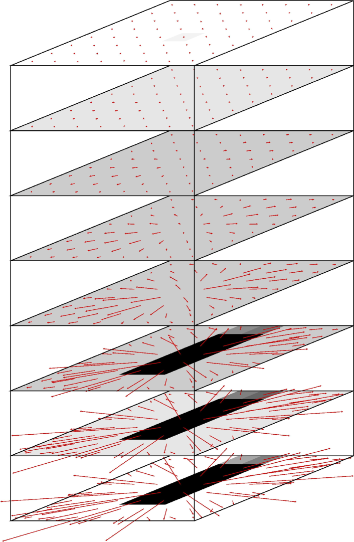
(a) Iter=0, U=6.18e17, $\tau=90.13\%$.

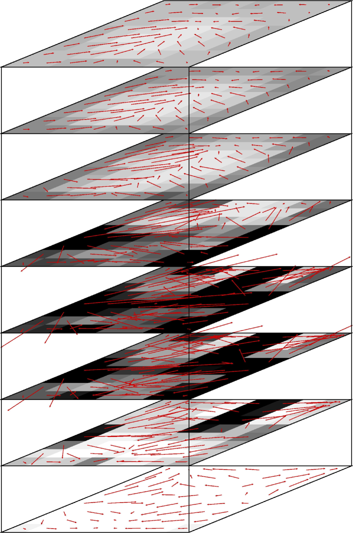
(b) Iter=3, U=5.84e16, $\tau=47.56\%$.

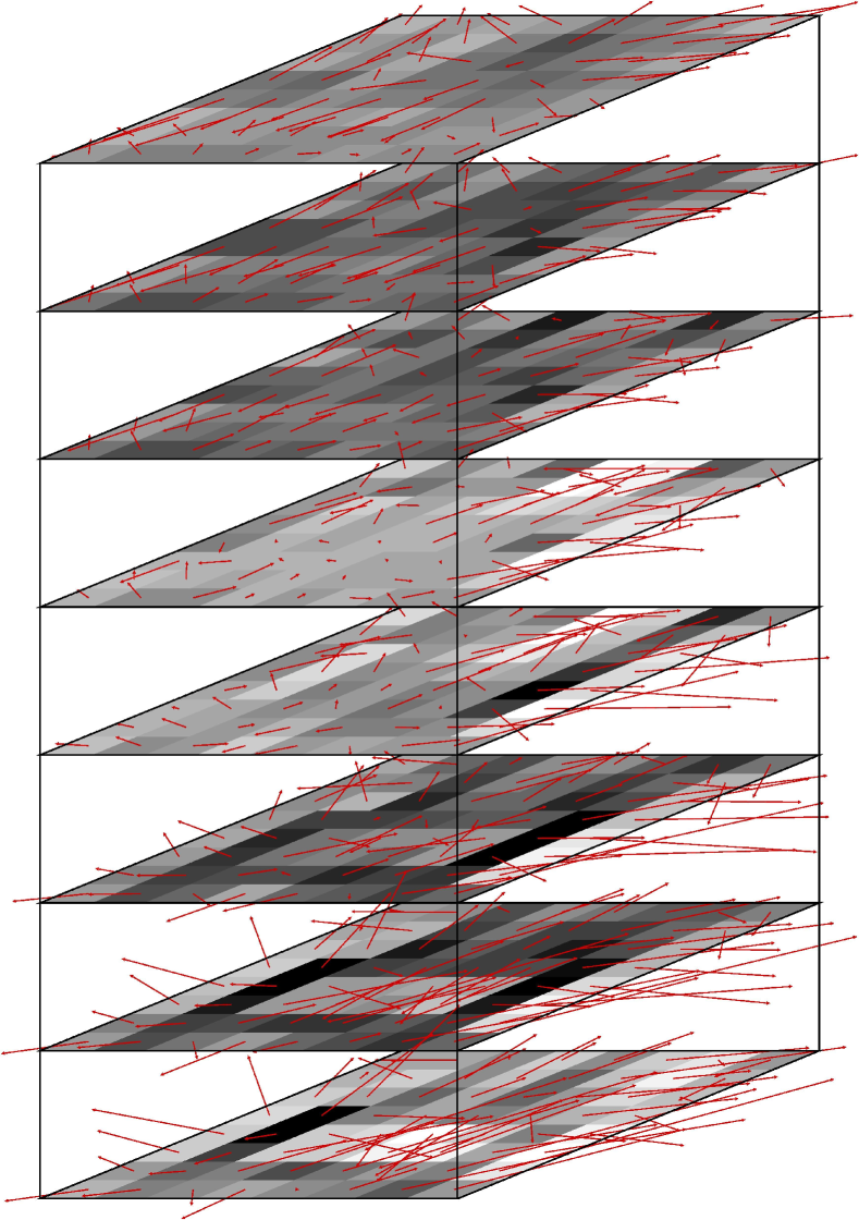
(c) Iter=6, U=3.56e15, $\tau=11.75\%$.

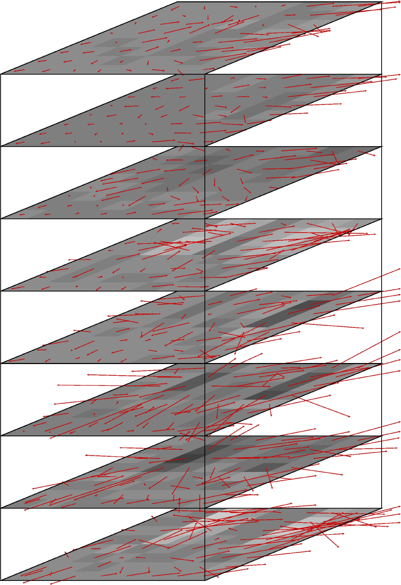
(d) Iter=20, U=2.07e14, $\tau=2.53\%$.

Figure 1: Iterative density-driven global placement (wirelength force disabled) with potential $U$ and density overflow $\tau$ on the MMS ADAPTEC1 benchmark with three tiers and resolution of $8\times 8\times 8$. Electric density and field are shown by gray scale and red arrows. All the movable objects are initialized at the bottom tier where all IO blocks locate. eDensity-3D iteratively spreads all the movable objects evenly within the entire 3D domain to equalize the placement density.

In this work, we extend the 2D placers ePlace [25, 23, 22] and ePlace-MS [26, 22] to the 3D domain. Our algorithm is named ePlace-3D and focused on wirelength minimization and density equalization, while other 3D-IC objectives like thermal are not covered. To the best of our knowledge, this is the first work in literature achieving analytically global smoothness along all the three dimensions. In contrast, previous analytic works [10, 27] only ensure (partially) local smoothness in their density functions [34, 12], while their less continuous cell movement would slow down placement convergence and cause more penalty on wirelength. We conduct analytic global placement and stochastic legalization in the entire 3D cuboid domain, which maximizes the search space thus further boost the solution quality. ePlace-3D well demonstrates the applicability of the electrostatic density model eDensity [24, 23] in various physical dimensions. Our specific contributions are listed as follows.

• eDensity-3D: an electrostatics based 3D density function ensuring global smoothness.

• A 3D numerical solution based on fast Fourier transform (FFT) and improved spectral formulation.

• A nonlinear 3D preconditioner to equalize all the moving objects in the optimization perspective.

• Interleaving coarse-grained 3D placement with fine-grained 2D placement to enhance efficiency.

• Our mixed-size 3D-IC placement prototype ePlace-3D outperforms the leading placers mPL6-3D [27] and NTUplace3-3D [10] with $6.44\%$ and $37.15\%$ shorter wirelength, $9.11\%$ and $10.27\%$ fewer 3D vertical interconnects, while runs $2.55\times$ and $0.30\times$ faster on average of all the ten IBM-PLACE benchmarks [13],

The remainder is organized as follows. Section 2 introduces the background knowledge. Section 3 discusses our 3D placement density function eDensity-3D, numerical solution, and nonlinear precondition. Section 4 provides an overview of ePlace-3D algorithm. Experiments and results are shown in Section 5. We conclude in Section 6.

2 Background

Given a set $V$ of $n$ objects, net set $N$ and 3D cuboid core region $R=[0,d_{x}]\times[0,d_{y}]\times[0,d_{z}]$, global placement is formulated as constrained optimization. The constraint desires all the objects to be accommodated with zero overlap. Let $\mathbf{v}$ denote the placement solution, which consists of the physical coordinates of all the objects. The region $R$ is uniformly decomposed into $m_{x}\times m_{y}\times m_{z}$ 3D bins denoted as set $B$. For every bin $b\in B$, the density $\rho_{b}(\mathbf{v})$ should not exceed the target density $\rho_{t}$. The objective is to minimize the total half-perimeter wirelength (HPWL) of all the nets. Let $HPWL_{e_{x}}=\max_{i,j\in e}|x_{i}-x_{j}|$ denote the horizontal wirelength of net $e$ (similar for $HPWL_{e_{y}}$), the total 2D HPWL is $HPWL(\mathbf{v})=\sum_{e\in N}\left(\beta_{x}HPWL_{e_{x}}(\mathbf{v})+\beta_{y}HPWL_{e_{y}}(\mathbf{v})\right)$. We use $\beta_{x}$, $\beta_{y}$ and $\beta_{z}$ as dimensional weighting factors. 3D-IC placement needs vertical interconnects, such as through-silicon via (TSV) and monolithic inter-tier via (MIV), to penetrate silicon tiers. Diverse types of connects have different physical and electrical properties. However, ePlace-3D is compatible with any types of connects, which can be reflected on the weight of $\beta_{z}$. In the remainder of this manuscript, we name all types of 3D vertical interconnects uniformly as $\mathbf{VI}$ for simplicity. The number of vertical interconnect units ($\#$VI) is computed as how many times silicon tiers have been penetrated, e.g., one vertical connect between tier one and tier three is counted as two $VI$. The nonlinear placement optimization is formulated as

$$\small\min_{\mathbf{v}}\text{ }\left(HPWL(\mathbf{v})+\beta_{z}\#VI\right)\text{ s.t. }\rho_{b}(\mathbf{v})\leq\rho_{t}\text{, }\forall b\in B.$$ (1)

Analytic methods conduct placement using gradient-directed optimization. As $HPWL(\mathbf{v})$ is not differentiable, we use wirelength smoothing by weighted-average (WA) model [10].

$$W_{e_{x}}(\mathbf{v})= \frac{\sum_{i\in e}x_{i}\exp\left(x_{i}/\gamma_{x}\right)}{\sum_{i\in e}\exp\left(x_{i}/\gamma_{x}\right)}-\frac{\sum_{i\in e}x_{i}\exp\left(-x_{i}/\gamma_{x}\right)}{\sum_{i\in e}\exp\left(-x_{i}/\gamma_{x}\right)}$$ (2)

Here $W_{e}(\mathbf{v})=\beta_{x}W_{e_{x}}(\mathbf{v})+\beta_{y}W_{e_{y}}(\mathbf{v})+\beta_{z}W_{e_{z}}(\mathbf{v})$ and $W(\mathbf{v})=\sum_{e}W_{e}(\mathbf{v})$. $\gamma_{x}$, $\gamma_{y}$ and $\gamma_{z}$ control the modeling accuracy. Density function relaxes all the $|B|$ constraints in Eq. (1). Most 2D and 3D quadratic placers [19, 18, 6] follow the linear density force formulation by [5]. Nonlinear placers [11, 1, 27, 10] have their dedicated density functions. NTUplace3-3D [10] leverages bell-shape curve [34] for local smoothness in 3D domain. mPL6-3D [1] uses Helmholtz function to globally smoothen the 2D plane and Huber’s function to locally smoothen the vertical dimension. The electrostatics based density function [25] converts objects to charges. By the Lorentz law, the electric repulsive force spreads charges away towards the electrostatic equilibrium state, which produces a globally even density distribution. Let $U(\mathbf{v})$ denote the density cost function, the constraints in Eq. (1) can be relaxed by the penalty factor $\lambda$, while the unconstrained optimization is shown as below.

$$\min_{\mathbf{v}}f(\mathbf{v})=W(\mathbf{v})+\lambda U(\mathbf{v}),\\$$ (3)

In this work, we set vertical connects as zero-volumed thus do not consider them in eDensity-3D. Therefore, the optimization of electrostatics will not be affected and can be still achieved based on the movement of netlist objects. Density overflow is used to terminate global placement and denoted as $\tau$, which is

$$\tau=\frac{\sum_{b\in B}\max\left(V^{m}_{b}-\rho_{t}V^{WS}_{b},0\right)}{V_{m}}.$$ (4)

Here $V_{m}$ is the total volume of all the movable objects, $V^{m}_{b}$ is the total volume of objects in the bin $b$, and $V^{WS}_{b}$ is the total whitespace in bin $b$. The volume of each cell is computed as its planar area multiplied by the depth of each tier.

3 eDensity-3D: 3D Density Function

In this section, we introduce our novel 3D density function eDensity-3D, a fast numerical solution by spectral methods, and approximated 3D nonlinear preconditioner. The key insight is, we treat the third dimension equally as the other two dimensions, such that vertical cell movement will be as smooth as the planar movement in 2D placement. The behavior of eDensity-3D is visualized in Figure 1.

3.1 3D Density Function

Extending the planar function eDensity in [25], eDensity-3D models the entire placement instance as a 3D electrostatic field. Every placement object (standard cells, macros and fillers) is converted to a positively charged cuboid. The electric repulsive force spreads all the objects away from the high-density region. The 3D density cost $U$ is modeled as the total potential energy of the system and defined as below

$$\scriptsize U(\mathbf{v})=\sum_{i\in V}U_{i}(\mathbf{v})=\sum_{i\in V}q_{i}\Phi_{i}(\mathbf{v}).$$ (5)

$q_{i}$ denotes the electric quantity of the charge $i$ and is set as the physical volume of placement object $i$. $\Phi_{i}$ is the electric potential at charge $i$. Charges with high potential will reduce the placement overlap by moving towards the direction of largest energy descent. Unlike the spatial density distribution $\rho(x,y,z)$ (Figure 1) which is coarse and non-differentiable, the electric potential distribution $\Phi(x,y,z)$ is globally smooth. We use the potential gradient (thus electric field), $\nabla\Phi(x,y,z)=\mathbf{E}(x,y,z)$, to direct cell movement for density equalization. Given a placement layout $\mathbf{v}$, we generate the density map $\rho(x,y,z)$, then compute the potential map $\Phi(x,y,z)$ by solving the 3D Poisson’s equation

$$\small\begin{cases}\nabla\cdot\nabla\Phi(x,y,z)=-\rho(x,y,z)\text{,}\\ \mathbf{\hat{n}}\cdot\nabla\Phi(x,y,z)=0\text{, }(x,y,z)\in\partial R,\\ \iiint\limits_{R}\Phi(x,y,z)=\iiint\limits_{R}\rho(x,y,z)=0\text{.}\\ \end{cases}$$ (6)

Here $\hat{n}$ is the outer unit normal of the placement cube $R$. $\partial R$ is the boundary and consists of orthogonal rectangular planes to enclose the placement cuboid. In Eq. (6), the first equation has $\nabla\cdot\nabla\equiv\frac{\partial^{2}}{\partial x^{2}}+\frac{\partial^{2}}{\partial y^{2}}+\frac{\partial^{2}}{\partial z^{2}}$. Neumann condition by the second equation requires that when any object $i$ reaches any boundary plane, its density force vector will have the component perpendicular to the plane reduced to zero, in order to prevent $i$ from penetrating the plane. The third equation shows that the integral of density $\rho(x,y,z)$ and potential $\Phi(x,y,z)$ within $R$ are set to zero to ensure that (1) electric force drives all the charges towards even density distribution rather than pushing them to infinity, which matches the placement objective (2) the 3D Poisson’s equation would have a unique solution by satisfying the Neumann condition. We differentiate the potential $\Phi_{i}$ on each charge $i$ to generate the electric field $\nabla\Phi_{i}=\mathbf{E_{i}}=\left(E_{i_{x}},E_{i_{y}},E_{i_{z}}\right)$. The electric (density) force is $\nabla U_{i}=q_{i}\nabla\Phi_{i}=q_{i}\mathbf{E_{i}}$.

3.2 3D Numerical Solution

Based on the 2D solution in [25], we solve the 3D Poisson’s equation by spectral methods using frequency decomposition [39]. To satisfy the Neumann condition of zero gradients at the boundaries, we use sinusoidal wave to express the electric field $\mathbf{E}(x,y,z)$. We construct an odd and periodic field distribution by negatively mirroring itself w.r.t. the origin, then periodically extending it towards positive and negative infinities. Electric potential and density distributions are then expressed by cosine waveforms, which are the integration and differentiation of the field. Let $a_{j,k,l}$ denote the 3D coefficients of the density frequency.

$$a_{j,k,l}=\frac{1}{n^{3}}\sum_{x,y,z}\rho(x,y,z)\cos(w_{j}x)\cos(w_{k}y)\cos(w_{l}z)$$ (7)

eDensity [25] sets $w_{j}=\pi\frac{j}{m_{x}}$, which equals the discrete index for the $j$th frequency component. However, as we are conducting placement in a continuous domain, the multiplication of $x$ and $w_{j}$ induces inconsistency. In this work, we propose improved spectral methods for the 3D placement density function. Specifically, we set $w_{j}=\pi\frac{j}{d_{x}}$ since $x$ ranges within $(0,d_{x})$. As a result, $w_{j}x=\pi j\frac{x}{d_{x}}$ well matches the original unit of discrete frequency index, and we have all the frequency indexes defined as $\{w_{j},w_{k},w_{l}\}=\{\frac{\pi j}{d_{x}},\frac{\pi k}{d_{y}},\frac{\pi l}{d_{z}}\}$. As mentioned in Section 2, here $d_{x}$, $d_{y}$ and $d_{z}$ represent the dimensions of the cuboid placement core region. $d_{\{x,y,z\}}$ can be set as any value since $w_{\{j,k,l\}}$ will be normalized by $\frac{\{x,y,z\}}{d_{\{x,y,z\}}}$. $j$, $k$ and $l$ range in $[0,n-1]$, which is only half of a cosine function period. In contrast, one complete function period centered at the origin is $[-n,n-1]$. Therefore, we have $\pi$ rather than $2\pi$ in the above frequency index. We set $a_{0,0,0}=0$ to remove the zero-frequency component. The spatial density distribution $\rho(x,y,z)$ is

$$\rho(x,y,z)= \sum_{j,k,l}a_{j,k,l}\cos(w_{j}x)\cos(w_{k}y)\cos(w_{l}z)\text{.}$$ (8)

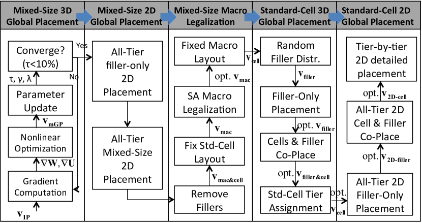
Figure 2: the flowchart of ePlace-3d.

To achieve $\nabla\cdot\nabla\Phi(x,y,z)=-\rho(x,y,z)$, the solution to the potential can be expressed as

$$\Phi(x,y,z)=\sum_{j,k,l}\frac{a_{j,k,l}}{w_{j}^{2}+w_{k}^{2}+w_{l}^{2}}\cos(w_{j}x)\cos(w_{k}y)\cos(w_{l}z).$$ (9)

By differentiating Eq. (9), we have the electric field distribution $\mathbf{E}(x,y,z)=(E_{x},E_{y},E_{z})$ shown as below

$$\begin{cases}E_{x}(x,y,z)=\sum_{j,k,l}\frac{a_{j,k,l}w_{j}}{w_{j}^{2}+w_{k}^{2}+w_{l}^{2}}\sin(w_{j}x)\cos(w_{k}y)\cos(w_{l}z),\\ E_{y}(x,y,z)=\sum_{j,k,l}\frac{a_{j,k,l}w_{k}}{w_{j}^{2}+w_{k}^{2}+w_{l}^{2}}\cos(w_{j}x)\sin(w_{k}y)\cos(w_{l}z),\\ E_{z}(x,y,z)=\sum_{j,k,l}\frac{a_{j,k,l}w_{l}}{w_{j}^{2}+w_{k}^{2}+w_{l}^{2}}\cos(w_{j}x)\cos(w_{k}y)\sin(w_{l}z).\\ \end{cases}$$ (10)

Let $|B|=m_{x}\times m_{y}\times m_{z}$ denote the total number of bins in global placement. Instead of quadratic complexity, above spectral equations can be efficiently solved using FFT algorithms [36] with $O\left(|B|log|B|\right)$ complexity.

3.3 3D Nonlinear Precondition

Theoretically, preconditioning improves convergence rate rather than solution quality. However, as placement is a highly nonlinear, non-convex and ill-conditioned problem, the Hessian matrix with improved condition number would reshape the search direction for the nonlinear solver to follow. As a result, preconditioning would open the gate for unexplored high-dimension search space, while surprising quality enhancement would be expectable.

Preconditioned mixed-size placement should tolerate the huge physical and topological differences between all the standard cells, macros, and dummy fillers. In [25], the nonlinear preconditioner $H$ for 2D placement is modeled as

$$\small H_{i_{x}}=\frac{\partial^{2}f}{\partial x_{i}^{2}}=\frac{\partial^{2}W}{\partial x_{i}^{2}}+\lambda\frac{\partial^{2}U}{\partial x_{i}^{2}}\approx|N_{i}|+\lambda A_{i}.$$ (11)

Here $N_{i}$ are all the nets incident to the object $i$, $A_{i}$ is the 2D area of the object $i$. In 3D placement, we use $V_{i}$ to denote the volume of $i$ instead. The preconditioned gradient $\nabla f_{pre}=H^{-1}\nabla f$ then improves and accelerates the placement. Our studies show that Eq. (11) relies on the assumption of $\frac{\partial^{2}W/\partial x_{i}^{2}}{\partial^{2}U/\partial x_{i}^{2}}\approx\frac{|N_{i}|}{A_{i}}$. However, the third dimension weakens $\frac{\partial^{2}W}{\partial x_{i}^{2}}$ and breaks the above assumption. As a result, $|N_{i}|$ dominates $\lambda V_{i}$ and makes fillers and macros with small $|N_{i}|$ spread faster than standard cells, as Eq. (12) shows

$$\scriptsize\left\|H_{i_{x}}^{-1}\nabla U\right\|=\left\|\frac{\partial U/\partial x_{i}}{\lambda V_{i}}\right\|\gg\left\|\frac{\partial f/\partial x_{i}}{|N_{i}|+\lambda V_{i}}\right\|=\left\|H_{i_{x}}^{-1}\nabla f\right\|.$$ (12)

Instead, we propose a new preconditioner as below

$$\small H_{i_{x}}=\frac{\partial^{2}f}{\partial x_{i}^{2}}\approx\lambda\frac{\partial^{2}U}{\partial x_{i}^{2}}\approx\lambda V_{i},$$ (13)

The noise factors introduced by $|N_{i}|$ is resolved, where all the objects are being equalized in the optimizer’s perspective and simultaneously spread over the entire domain. Experiments show that our 3D preconditioner reduces the global placement iterations by $15\%$ and improves the wirelength by $30\%$ over all the 16 MMS benchmarks.

3.4 Complexity

Complexity significantly impacts the placement runtime. In each iteration, we traverse all the bins to reset their density in $O(|B|)$ time, then traverse all the placement objects in $O(n)$ time to update the superimposed density map. By Eq. (7), (9) and (10), five times of 3D FFT computation are invoked, which costs $O(5n\log n)$ time. By our grid sizing strategy in Eq. (14), $|B|/n$ is limited to constant. The overall complexity is thus $O(|B|+n+5n\log n)\approx O(n\log n)$,

In ePlace-3D, the placement domain is geometrically transformed from $R=[0,d_{x}]\times[0,d_{y}]\times[0,d_{z}]$ to $R^{\prime}=[0,1]\times[0,1]\times[0,1]$. We set the density resolutions $m_{x}=m_{y}=m_{z}=m_{3D}$ to make the placement domain $R^{\prime}$ uniformly decomposed into $|B|=m_{3D}^{3}$ cubic bins. Let $V_{R}$ denote the total volume of $R$ and $V_{C_{avg}}$ denote the average area of all standard cells. The grid sizing is set as

$$\scriptsize|B|=\frac{V_{R}}{k\times V_{C_{avg}}\times\rho_{t}^{-1}}.$$ (14)

Here every $k$ standard cells are accommodated by one bin. Placement quality (efficiency) is determined by the value of $k$. In this work, we constantly set $k=1.0$.

4 ePlace-3D: Overview

ePlace-3D is built upon the infrastructure of ePlace-MS [26]. Figure 2 shows the flowchart of our algorithm. Given a placement instance, our algorithm minimizes the quadratic wirelength over the 3D domain to produce the initial solution $\mathbf{v_{IP}}$. To approach the optimum solution in the end, we make $\mathbf{v_{IP}}$ as minimum-wirelength violation-tolerant.

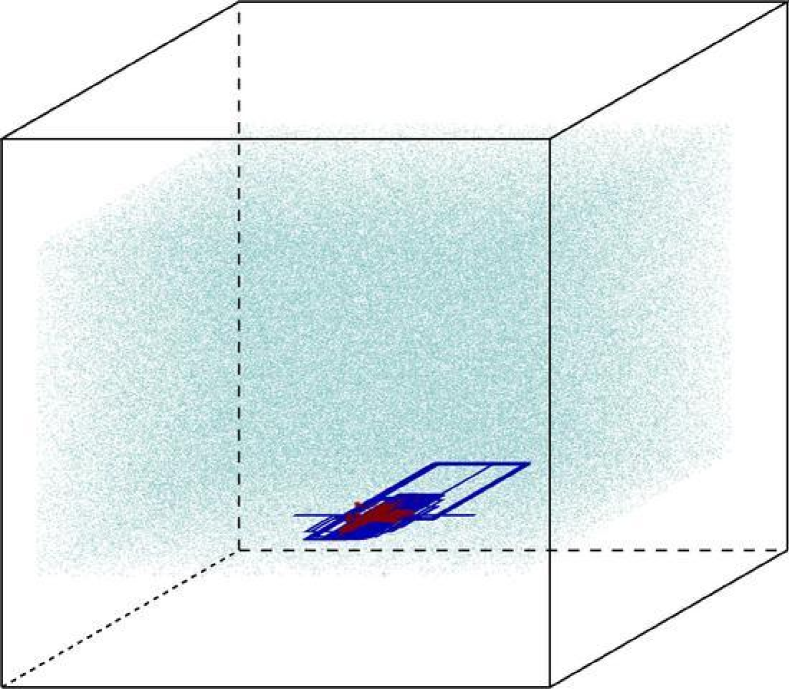
(a) Iter=0, WL=1.32e7, $\#$VI=0, $\tau=93.7\%$.

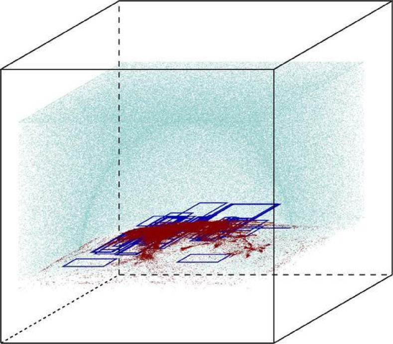
(b) Iter=266, WL=3.29e7, $\#$VI=1.35e3, $\tau=77.1\%$.

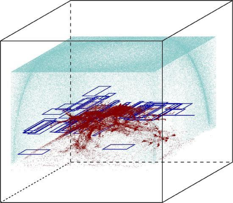
(c) Iter=328, WL=3.91e7, $\#$VI=4.14e3, $\tau=61.1\%$.

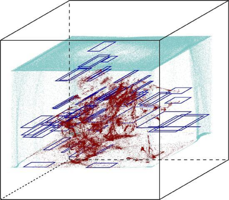
(d) Iter=376, WL=4.21e7, $\#$VI=7.70e3, $\tau=45.2\%$.

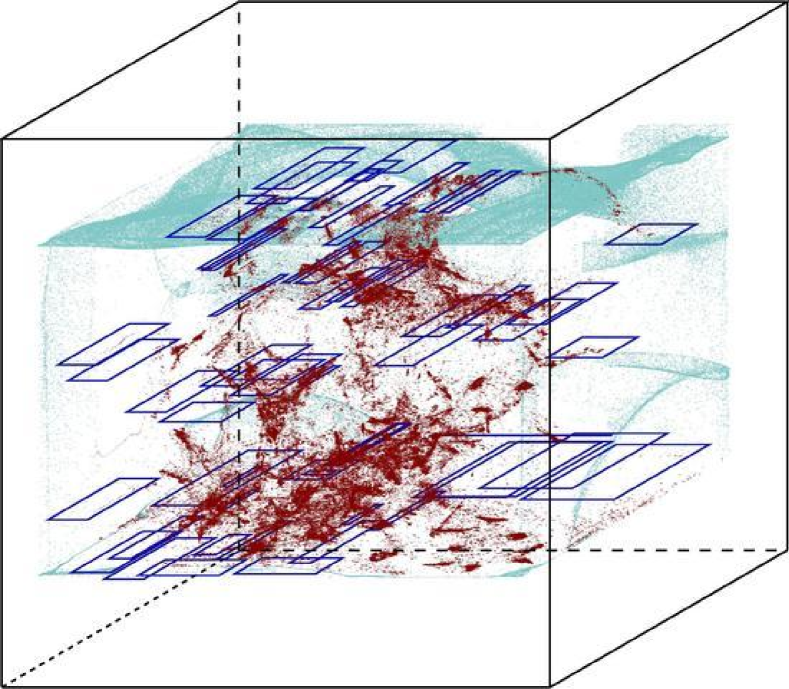
(e) Iter=432, WL=4.64e7, $\#$VI=8.57e3, $\tau=28.9\%$.

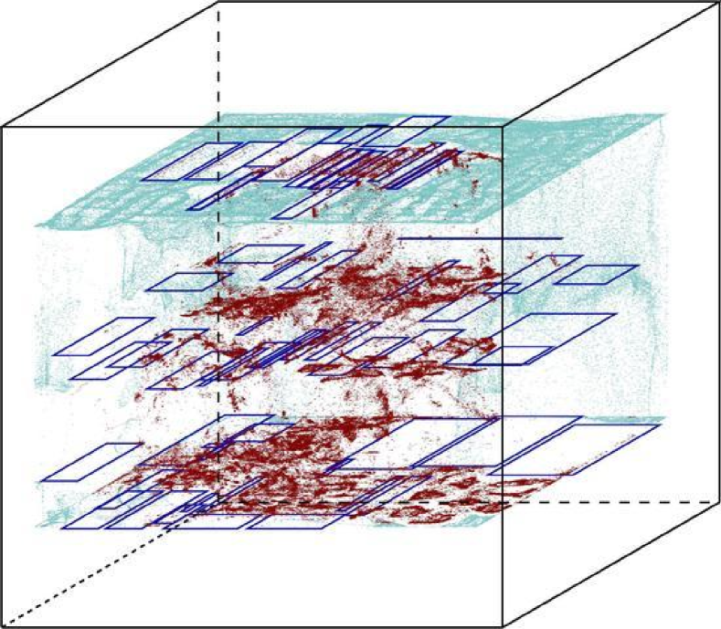
(f) Iter=481, WL=5.06e7, $\#$VI=8.70e3, $\tau=14.9\%$.

Figure 3: 3D-IC mixed-size global placement on MMS ADAPTEC1 with three tiers. Standard cells, macros and fillers are denoted by red dots, blue rectangles and cyan dots.

Our 3D-IC global placement is visualized in Figure 3. Unconnected fillers [1, 25] are inserted to populate up extra whitespace. All the fillers are equally sized by the average dimensions of all the standard cells. The optimum solution of 3D global placement will have all the cells, macros and fillers orient towards discrete tiers. Otherwise, some cuboid placement sites will be partially wasted, degrading the solution quality. Figure 3(f) illustrates the beauty of our approach, i.e., the analytic 3D placer is visually approaching density evenness from the vertical dimension, which ensures negligible quality overhead during tier assignment. We use Nesterov’s method [35] as the nonlinear solver and determine the steplength by [25].

A multi-tier 2D-IC mixed-size global placement follows by assigning all the macros and standard cells to the closest tiers and separately filling the remaining whitespace on each tier with fillers. Planar placement is conducted simultaneously over all the tiers. As wirelength smoothing is homogeneous over all the tiers (with the same $\gamma$), heterogeneous grid sizing is not feasible as density force is dependent on resolution by Eq. (10). We set all the tiers with the same density resolution $m_{2D}$, which is the maximum of that of all the tiers by Eq. (14) with $k=1$. In practice, we have $O(m^{2}_{2D})\approx O(m_{3D}^{3})$. Figure 4 illustrates the progression.

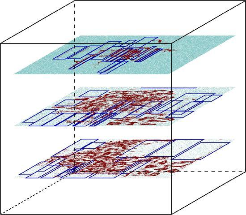
(a) Iter=0, WL=4.71e7, $\#$VI=7.96e3, $\tau=31.9\%$.

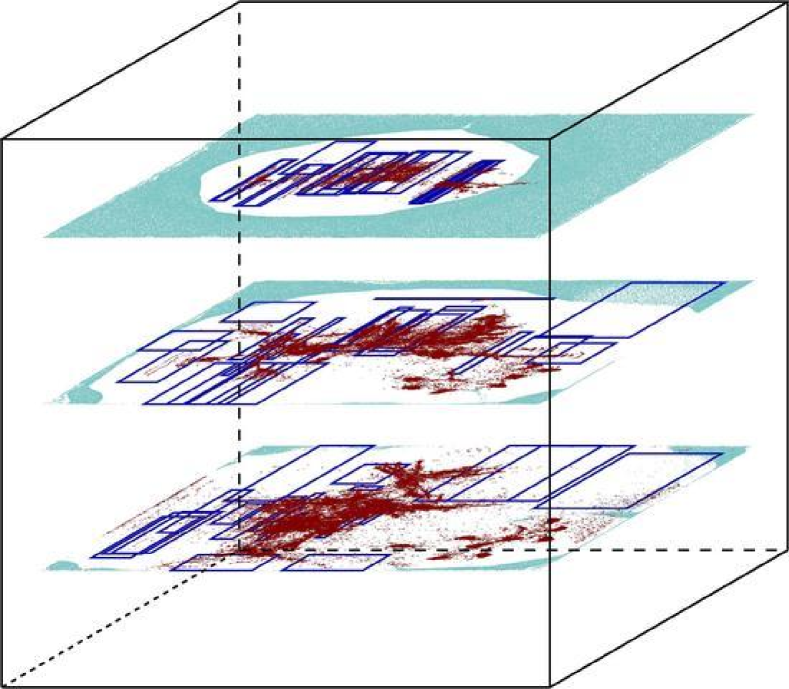
(b) Iter=246, WL=3.64e7, $\#$VI=7.96e3, $\tau=50.3\%$.

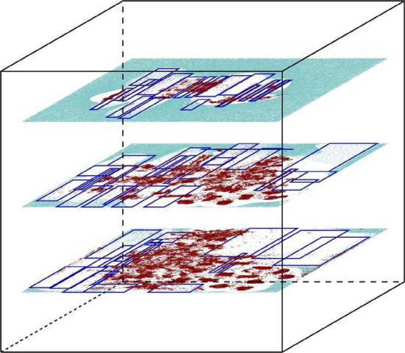
(c) Iter=322, WL=4.46e7, $\#$VI=7.96e3, $\tau=31.9\%$.

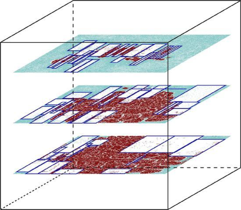
(d) Iter=395, WL=4.99e7, $\#$VI=7.96e3, $\tau=14.8\%$.

Figure 4: 2D-IC mixed-size global placement on MMS ADAPTEC1 with three tiers. Initial and final overflow are both larger than the final overflow of 3D placement due to finer granularity ($m_{2D}\gg m_{3D}$).

Our 3D-IC macro legalizer generates a legal macro layout with zero macro overlap and small wirelength overhead. The algorithm is stochastic based on simulated annealing [20]. A 3D-IC standard-cell global placement follows to mitigate the quality loss due to sub-optimal macro legalization. We assign standard cells to their closest tiers and conduct simultaneous 2D-IC standard-cell placement on all the tiers. The standard-cell layouts of all the tiers are locally refined. Figure 5 shows the respective placement progressions, more details can be found in [26]. The detailed placer from [37] is then invoked for a tier-by-tier standard-cell legalization and detailed placement from the bottom to the top tier.

Table 1: HPWL (e7), $\#$VI (vertical interconnect) (e3) and runtime (minutes) on the IBM-PLACE benchmark suite [13]. Cited results are marked with ^∗. All the experiments are conducted under single-thread mode. The results are evaluated by the same scripts and normalized to ePlace-3D. The best result for each case is in bold-face.

Categories			NTUplace3-3D [10]			mPL6-3D∗ [27]			ePlace-3D
Benchmarks	$\#$ Cells	$\#$ Nets	HPWL	$\#$VI	CPU	HPWL	$\#$VI	CPU	HPWL	$\#$VI	CPU
IBM01	12K	12K	0.34	0.69	0.20	0.26	1.04	2.95	0.25	1.31	0.58
IBM03	22K	22K	0.76	3.32	0.50	0.59	3.11	4.72	0.56	3.27	1.33
IBM04	27K	26K	1.00	2.60	0.60	0.81	2.95	6.41	0.74	3.53	1.88
IBM06	32K	33K	1.30	3.99	0.80	1.05	3.97	6.20	0.92	4.50	2.98
IBM07	45K	44K	1.92	5.73	1.30	1.59	4.68	8.64	1.50	4.39	3.87
IBM08	51K	48K	2.08	4.90	1.70	1.71	3.94	11.23	1.54	4.90	4.75
IBM09	52K	50K	1.92	3.88	1.50	1.45	3.24	14.61	1.40	3.18	5.63
IBM13	82K	84K	3.69	3.98	2.60	2.88	5.59	19.62	2.67	4.73	8.65
IBM15	158K	161K	9.16	15.67	7.20	6.79	10.52	46.82	6.39	9.16	40.25
IBM18	210K	201K	13.41	12.19	13.60	9.16	15.22	52.09	9.47	6.83	63.07
Avg.	69K	68K	$37.15\%$	$10.27\%$	$0.30\times$	$6.44\%$	$9.11\%$	$2.55\times$	$0.00\%$	$0.00\%$	$1.00\times$

In general, we have fine-grained 2D placement interleaved with coarse-grained 3D placement, which achieves a good trade-off between quality and efficiency. On average of all the ten IBM-PLACE circuits, the application of 2D refinement reduces the wirelength by more than $4\%$.

5 Experiments and Results

We implement ePlace-3D using C programming language in the single-thread mode and execute the program in a Linux machine with Intel i7 920 2.67GHz CPU and 12GB memory. There is no benchmark specific parameter tuning in our work. $\#$VI are controlled by the weighting factor $\beta_{z}$ based on capacitance ratio. By [16], one TSV (VI) has the capacitance of $C_{VI}=30fF$ at 45nm tech-node. ITRS annual reports [14] show that unit capacitance of interconnects at intermediate routing layers is constantly $2pF/cm$ across various tech-nodes. Placement row height is $1.4um$ at 45nm tech-node ($70nm$ M1 half-pitch, ten M1 tracks per row), capacitance becomes $C_{ROW}=0.3fF$ for 2D interconnect spanning one-row height. Based on the length units for each benchmark, as well as our geometric transformation of the placement core region to be $[0,1]\times[0,1]\times[0,1]$ as discussed in Section 3.4, we compute the respective capacitance ratio of one VI versus one unit wirelength and use it as the VI weight. Specifically, we have

$$\beta_{z}=\frac{\#tiers\times C_{VI}}{\#rows\times C_{ROW}}\\$$ (15)

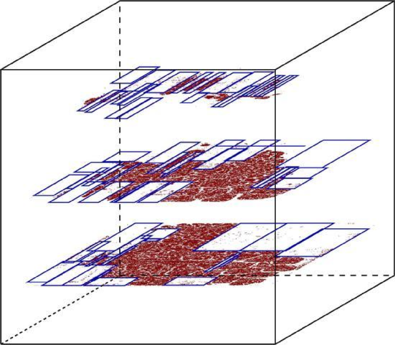
(a) 3D macro LG: iter=0, WL=4.99e7, $\#$VI=7.96e3, Om=9.05e5.

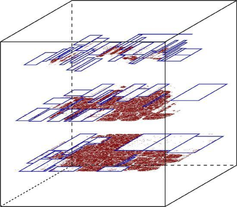
(b) 3D macro LG: iter=4, WL=5.10e7, $\#$VI=9.10e3, Om=0.

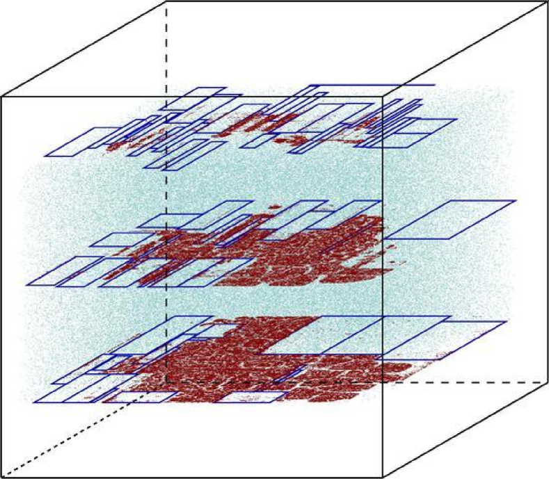
(c) 3D standard-cell GP: iter=0, WL=5.10e7, $\#$VI=9.10e3, $\tau=8.1\%$.

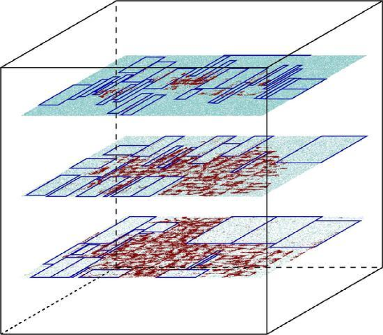
(d) 2D standard cell GP: iter=0, WL=4.92e7, $\#$VI=9.10e3, $\tau=66.7\%$.

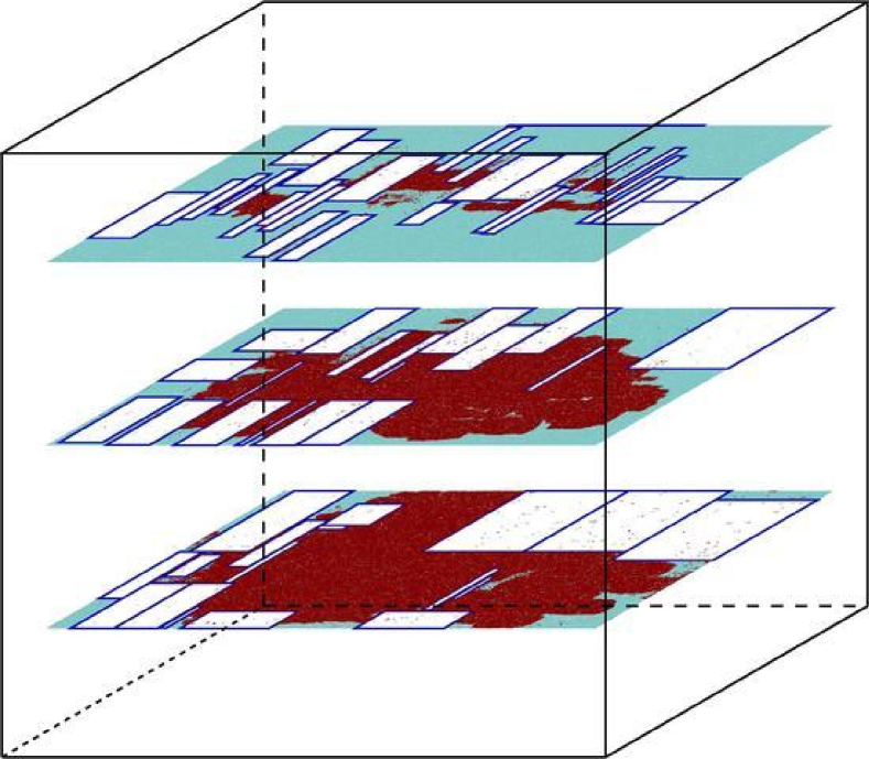
(e) 2D standard cell GP: iter=394, WL=5.08e7, $\#$VI=9.11e3, $\tau=14.8\%$.

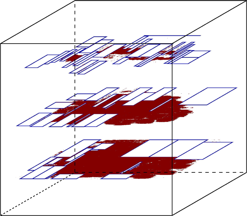
(f) 2D standard cell DP: WL=5.42e7, $\#$VI=9.10e3, $\tau=0\%$.

Figure 5: Post-placement on MMS ADAPTEC1 with three tiers. Standard cells, macros and fillers are denoted by red dots, blue rectangles and cyan dots. Om denotes the total macro overlap.

Notice that the focus of this work is the algorithm framework of 3D placement, not the accurate weight modeling of vertical connects. The weighting factor can be adjusted by VLSI designers for their particular needs, e.g., vertical connects of different electric and physical attributes (TSVs, MIVs, super contacts, etc.).

We conduct experiments on IBM-PLACE [13] standard-cell benchmarks without macros or blockages, all of which are derived from real IC design. We include two state-of-the-art 3D-IC placers, mPL6-3D [27], and NTUplace3-3D [10], in our experiments on IBM-PLACE. As other categories of algorithms (e.g., folding and partition based approaches) have been outperformed by analytic placement in literature, we do not include them in our experiments. We have obtained the binary of NTUplace3-3D from the original authors and executed it on our machine for experiments. mPL6-3D is not available (as notified by the author), so we cite the performance from their latest publication [27]. We use exactly the same benchmark transformation as that by mPL6-3D and NTUplace3-3D. I.e., we insert four silicon tiers into each benchmark, scale down each tier to $\frac{1}{4}$ of the original 2D placement area, add $10\%$ whitespace to each tier, and keep the aspect ratio of each tier to be the same as the original 2D design. As a result, all the experiments on the three placers, including those from [27], are conducted on exactly the same IBM-PLACE-3D benchmarks. As HPWL and $\#$VI are being computed in exactly the same way, the performance comparison among the three placers are fair. The results on IBM-PLACE cases are shown in Table 1. On average of all the ten circuits, ePlace-3D outperforms mPL6-3D and NTUplace3-3D with $6.44\%$ and $37.15\%$ shorter wirelength together with $9.11\%$ and $10.27\%$ fewer VIs. ePlace-3D runs $2.55\times$ faster than mPL6-3D but $0.30\times$ slower than NTUplace3-3D, nevertheless, the improvement on wirelength ($37.15\%$) and VI ($10.27\%$) is significant.

Table 2: HPWL (e6), $\#$VI (vertical interconnect) and runtime (mins) on MMS circuits. Cited results are marked with ^∗. All the experiments are in single-thread mode. The HPWL and CPU results are normalized to the best published 2D placement results [26], $\#$VI are normalized to $\#$ objects.

$\#$ tiers			ePlace-MS∗ [26]		ePlace-3D w/ 2 tiers			ePlace-3D w/ 3 tiers			ePlace-3D w/ 4 tiers
Benchmarks	$\#$ Objs	$\#$ Nets	HPWL	CPU	HPWL	$\#$VI	CPU	HPWL	$\#$VI	CPU	HPWL	$\#$VI	CPU
ADAPTEC1	211K	221K	67.15	5.47	59.51	5733	24.63	54.19	9104	14.65	51.3	13568	16.03
ADAPTEC2	255K	266K	77.37	7.43	73.97	9269	39.67	75.38	9929	25.18	59.97	18085	24.57
ADAPTEC3	451K	466K	164.50	27.23	141.97	5557	95.48	136.85	18203	88.55	120.29	28694	94.42
ADAPTEC4	496K	515K	148.38	29.35	126.94	8149	107.15	113.22	13811	121.40	106.34	14527	118.13
BIGBLUE1	278K	284K	86.82	7.82	76.06	8272	40.63	71.34	10508	36.17	63.64	19403	38.05
BIGBLUE2	557K	577K	130.18	13.70	109.27	2565	70.25	97.1	5347	63.58	90.14	9241	64.95
BIGBLUE3	1096K	1123K	302.29	72.98	251.77	24466	268.47	271.27	42053	291.38	295.38	62669	388.08
BIGBLUE4	2177K	2229K	657.92	204.15	577.98	21263	491.97	537.2	50552	563.98	500.25	113590	420.17
ADAPTEC5	843K	867K	310.54	48.35	258.18	22705	170.90	244.57	27764	146.22	223.44	50732	149.22
NEWBLUE1	330K	338K	61.85	10.87	56.36	5901	28.15	53.05	7295	24.08	48.85	12346	25.07
NEWBLUE2	441K	465K	162.93	62.40	179.82	25571	67.27	143.5	43642	77.20	169.78	53487	72.98
NEWBLUE3	494K	552K	304.15	17.53	240.47	7686	308.62	365.10	48979	410.73	397.46	51597	265.67
NEWBLUE4	646K	637K	228.54	29.73	197.21	11372	110.02	177.82	29767	112.80	171.21	35067	101.78
NEWBLUE5	1233K	1284K	392.27	63.40	344.95	45995	202.12	303.05	64336	195.52	280.42	95768	216.22
NEWBLUE6	1255K	1288K	408.36	69.65	379.59	10901	222.72	325.35	50487	194.57	298.82	66983	180.88
NEWBLUE7	2507K	2636K	894.31	191.47	814.79	18615	363.30	696.27	92943	375.65	670.51	111562	353.92
Avg.	829K	859K	$0.00\%$	$1.00\times$	$13.67\%$	$2.17\%$	$3.13\times$	$20.50\%$	$4.30\%$	$3.03\times$	$27.54\%$	$6.10\%$	$2.94\times$

To validate the scalability of ePlace-3D, we also conduct experiments on the large-scale modern mixed-size (MMS) benchmarks [43] with on average 829K and up to 2.5M netlist objects. MMS benchmarks was first published in DAC 2009. The circuits inherit the same netlists and density constraints $\rho_{t}$ from ISPD 2005 [33] and ISPD 2006 [32] benchmarks but have all the macros freed to place. The original planar placement domain is geometrically transformed to be of $2$, $3$ and $4$ silicon tiers, each tier is equally downsized to keep both the aspect ratio and total silicon area unchanged. All the standard cells and macros keep their original dimensions and span only one tier. MMS circuits have all their fixed objects with zero area (volume) and outside the placement boundaries, and we geometrically transform them to the boundary of the bottom (first) tier. Also, as macros are all free to move, we skip the geometrical transformation of the fixed macro layout from 2D to 3D, which is sub-optimal and usually causes quality loss. Similar to mPL6-3D [27] and NTUplace3-3D [10], we add $10\%$ extra whitespace to each tier, in order to relieve the placement dilemma due to the increased area ratio between large macros and silicon tiers. There are benchmark-dependent target density $\rho_{t}$ for eight out of the sixteen MMS circuits. Detailed circuit statistics can be found in Table 1 of [43]. We create evaluation scripts to compute the total wirelength, number of vertical interconnects, and legality of the produced 3D-IC placement solution. The results on the MMS benchmarks are shown in Table 2. Notice that here HPWL is the original half-perimeter wirelength. It is not penalized by the amount of density overflow, since the density overflow in 3D domain is of one more dimension thus hard to compare with that of 2D domain. The binary of NTUplace3-3D does not work with these benchmarks, while the binary of mPL6-3D is not available for use. As a result, we compare the 3D MMS placement solutions with the best published (golden) 2D results in literature [26]. By using two, three and four tiers, ePlace-3D outperforms the golden 2D placement with on average $13.67\%$, $20.50\%$ and $27.54\%$ shorter wirelength. On the other side, the average ratio between the number of vertical interconnect units versus the number of placement objects (standard cells and macros) are only $2.17\%$, $4.30\%$ and $6.10\%$, respectively. These vertical connect ratios are much smaller than the average VI ratio on IBM-PLACE, which are more than $9\%$ for all the three placers in Table 1. Due to the introduction of the third dimension, the search space of placement optimization is substantially enlarged. However, the runtime increase is just $3\times$, which indicates high efficiency of ePlace-3D.

We also study the trends of HPWL and $\#$VI by linearly sweeping the number of tiers and exponentially sweeping the VI weight. We select eight out of the sixteen MMS benchmarks (ADAPTEC1, ADAPTEC4, BIGBLUE1, BIGBLUE2, BIGBLUE3, BIGBLUE4, NEWBLUE6, NEWBLUE7), all of which could accommodate the maximum macro block after inserting ten tiers. Keeping the same aspect ratio, the area of each tier is scaled down by ten times with the insertion of $10\%$ extra whitespace. Figure 6 shows that ePlace-3D is able to reduce the total 2D wirelength by up to $40\%$ (with the insertion of up to ten tiers), while $\#$VI is roughly scaled up by the number of tiers.

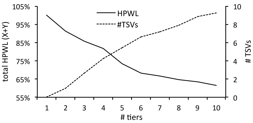
Figure 6: Avg. HPWL and $\#$VI of eight selected MMS cases w.r.t. number of silicon tiers.

VI weight sweeping is conducted on all the sixteen MMS benchmarks. Figure 7 shows the trends of average HPWL and $\#$VI by dividing the normal VI weight by up to 32 times (i.e. $\times$ 0.03125). The total 2D HPWL saturates at the reduction of $7\%$, while $\#$VI is scaled up by roughtly $2.5\times$.

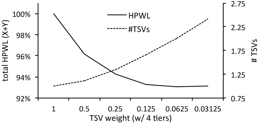
Figure 7: Avg. HPWL and $\#$VI of all the sixteen MMS cases w.r.t. VI weights.

Our 3D-IC placement algorithm shows significant quality improvement while limited runtime overhead. BIGBLUE4 and NEWBLUE7 are the largest circuits with 2.2M and 2.5M cells, and they consume the longest runtime on the 3D-IC placement. However, compared to the respective golden 2D placement solutions, the runtime ratio is upper-bounded by $2.5\times$, which is still less than the average runtime ratios of $3.13\times$ for two tiers, $3.03\times$ for three tiers and $2.94\times$ for four tiers, respectively. To this end, ePlace-3D shows good scalability and acceptable efficiency on the large cases.

In this work, we do not test ePlace-3D on circuits with fixed macros, as geometrically transforming the 2D floorplan into 3D is difficult and usually error-prone. However, ePlace-3D shows high performance and scalability on MMS benchmarks with lots of movable large macros, which is more difficult to place than fixed-macro layouts. As a result, we are confident on the performance of ePlace-3D on any circuits with fixed macros. The advantage of 3D tier insertion vanishes if there are large macros to accommodate (BIGBLUE3, NEWBLUE3, etc.). Transformation of 2D planar macros into 3D cuboid macros would resolve this issue and ensure the consistent benefits by inserting more tiers. However, it is beyond this work and will be covered in future.

6 Conclusion

We propose the first electrostatics based placement algorithm ePlace-3D, which is effective and efficient for 3D-ICs with uniform exploration over the entire 3D space. Our 3D-IC density function leverages the analogy between placement spreading and electrostatic equilibrium, while global and uniform smoothness is realized at all the three dimensions. Our balancing and preconditioning techniques prevent solution oscillation or divergence. The interleaved 3D coarse-grained optimization followed by 2D fine-grained post processing obtains a good trade-off between quality and efficiency. The experimental results validate the high performance and scalability of our approach, indicating the benefits of placement smoothness. In future, we will develop 3D density function to address the volume of vertical interconnects (VI). We would also like to explore advanced technology for 3D-IC placement/routing with patterning and graph coloring technology [21].

7 Acknowledgment

The authors acknowledge (1) Prof. Dae Hyun Kim and Prof. Sung Kyu Lim for providing the 3D-IC flow scripts and IWLS testcases (2) Dr. Meng-Kai Hsu and Prof. Yao-Wen Chang for providing the binary of NTUplace3-3D (3) Dr. Guojie Luo and Prof. Jason Cong for providing the binary of mPL6-3D (4) the support of NSF CCF-1017864.

References

- [1] T. F. Chan, J. Cong, J. R. Shinnerl, K. Sze, and M. Xie. mPL6: Enhanced Multilevel Mixed-Size Placement. In ISPD, pages 212–214, 2006.
- [2] T.-C. Chen, Z.-W. Jiang, T.-C. Hsu, H.-C. Chen, and Y.-W. Chang. NTUPlace3: An Analytical Placer for Large-Scale Mixed-Size Designs with Preplaced Blocks and Density Constraint. IEEE TCAD, 27(7):1228–1240, 2008.
- [3] Y.-G. Chen, T. Wang, K.-Y. Lai, W.-Y. Wen, Y. Shi, and S.-C. Chang. Critical Path Monitor Enabled Dynamic Voltage Scaling for Graceful Degradation in Sub-Threshold Designs. In DAC, pages 1–6, 2014.
- [4] J. Cong, G. Luo, J. Wei, and Y. Zhang. Thermal-Aware 3-D IC Placement Via Transformation. In ASPDAC, pages 780–785, 2007.
- [5] H. Eisenmann and F. M. Johannes. Generic Global Placement and Floorplanning. In DAC, pages 269–274, 1998.
- [6] B. Goplen and S. Sapatnekar. Efficient Thermal Placement of Standard Cells in 3D ICs using a Force Directed Approach. In ICCAD, 2003.
- [7] B. Goplen and S. Sapatnekar. Placement of 3-D ICs with Thermal and Interlayer Via Considerations. In DAC, pages 626–631, 2007.
- [8] S. K. Han, K. Jeong, A. B. Kahng, and J. Lu. Stability and Scalability in Global Routing. In SLIP, pages 1–6, 2011.
- [9] Q. He, D. Chen, and D. Jiao. From Layout Directly to Simulation: A First-Principle Guided Circuit Simulator of Linear Complexity and Its Efficient Parallelization. IEEE CPMT, 2(4):687–699, 2012.
- [10] M.-K. Hsu, V. Balabanov, and Y.-W. Chang. TSV-Aware Analytical Placement for 3D IC Designs Based on a Novel Weighted-Average Wirelength Model. IEEE TCAD, 32(4):497–509, 2013.
- [11] M.-K. Hsu and Y.-W. Chang. Unified Analytical Global Placement for Large-Scale Mixed-Size Circuit Designs. IEEE TCAD, 2012.
- [12] P. J. Huber. Robust Statistics. John Wiley and Sons, 1981.
- [13] IBM-PLACE. http://er.cs.ucla.edu/benchmarks/ibm-place. 2001.
- [14] ITRS. http://www.itrs.net/Links/2012ITRS/Home2012.htm. 2012.
- [15] IWLS. http://iwls.org/iwls2005/benchmarks.html. 2005.
- [16] M. Jung et al. How to Reduce Power in 3D IC Designs: A Case Study with OpenSPARC T2 Core. In CICC, 2013.
- [17] A. B. Kahng and Q. Wang. A Faster Implementation of APlace. In ISPD, pages 218–220, 2006.
- [18] D. H. Kim, K. Athikulwongse, and S. K. Lim. A Study of Through-Silicon-Via Impact on the 3-D Stacked IC Layout. In ICCAD, 2009.
- [19] M.-C. Kim and I. Markov. ComPLx: A Competitive Primal-dual Lagrange Optimization for Global Placement. In DAC, 2012.
- [20] S. Kirkpatrick, C. D. G. Jr., and M. P. Vecchi. Optimization by Simulated Annealing. Science, 220(4598):671–680, 1983.
- [21] W. Lin, M. McGrath, I. Ramzy, T. H. Lai, and D. Lee. Detecting Job Interference in Large Distributed Multi-Agent Systems - A Formal Approach. In IEEE IM, 2013.
- [22] J. Lu. Analytic VLSI Placement using Electrostatic Analogy. Ph.D. Dissertation, University of California, San Diego, 2014.
- [23] J. Lu, P. Chen, C.-C. Chang, L. Sha, D. Huang, C.-C. Teng, and C.-K. Cheng. ePlace: Electrostatics based Placement using Fast Fourier Transform and Nesterov’s Method. ACM TODAES, 20(2):article 17, 2015.
- [24] J. Lu, P. Chen, C.-C. Chang, L. Sha, D. J.-H. Huang, C.-C. Teng, and C.-K. Cheng. FFTPL: An Analytic Placement Algorithm Using Fast Fourier Transform for Density Equalization. In ASICON, pages 1–4, 2013.
- [25] J. Lu, P. Chen, C.-C. Chang, L. Sha, D. J.-H. Huang, C.-C. Teng, and C.-K. Cheng. ePlace: Electrostatics based Placement using Nesterov’s Method. In DAC, pages 1–6, 2014.
- [26] J. Lu, H. Zhuang, P. Chen, H. Chang, C.-C. Chang, Y.-C. Wong, L. Sha, D. Huang, Y. Luo, C.-C. Teng, and C.-K. Cheng. ePlace-MS: Electrostatics based Placement for Mixed-Size Circuits. IEEE TCAD, 34(5):685–698, 2015.
- [27] G. Luo, Y. Shi, and J. Cong. An Analytical Placement Framework for 3-D ICs and Its Extension on Thermal Awareness. IEEE TCAD, 2013.
- [28] P.-W. Luo, T. Wang, C.-L. Wey, L.-C. Cheng, B.-L. Sheu, and Y. Shi. Reliable Power Delivery System Design for Three-Dimensional Integrated Circuits (3D ICs). In ISVLSI, pages 356–361, 2012.
- [29] I. L. Markov, J. Hu, and M.-C. Kim. Progress and Challenges in VLSI Placement Research. In DAC, 2012.
- [30] J. Miao, A. Gerstlauer, and M. Orshansky. Approximate Logic Synthesis under General Error Magnitude and Frequency Constraints. In ICCAD, pages 779–786, 2013.
- [31] J. Miao, A. Gerstlauer, and M. Orshansky. Multi-Level Approximate Logic Synthesis under General Error Constraints. In ICCAD, pages 504–510, 2014.
- [32] G.-J. Nam. ISPD 2006 Placement Contest: Benchmark Suite and Results. In ISPD, pages 167–167, 2006.
- [33] G.-J. Nam et al. The ISPD2005 Placement Contest and Benchmark Suite. In ISPD, pages 216–220, 2005.
- [34] W. C. Naylor, R. Donelly, and L. Sha. Non-Linear Optimization System and Method for Wire Length and Delay Optimization for an Automatic Electric Circuit Placer. In US Patent 6301693, 2001.
- [35] Y. E. Nesterov. A Method of Solving A Convex Programming Problem with Convergence Rate . Soviet Math, 27(2):372–376, 1983.
- [36] T. Ooura. General Purpose FFT Package, http://www.kurims.kyoto-u.ac.jp/~ooura/fft.html. 2001.
- [37] M. Pan, N. Viswanathan, and C. Chu. An Efficient and Effective Detailed Placement Algorithm. In ICCAD, pages 48–55, 2005.
- [38] C.-W. Sham, E. F.-Y. Young, and J. Lu. Congestion Prediction in Early Stages of Physical Design. ACM TODAES, 14(1):12:1–18, 2009.
- [39] G. Skollermo. A Fourier Method for the Numerical Solution of Poisson’s Equation. Mathematics of Computation, 29(131):697–711, 1975.
- [40] P. Spindler, U. Schlichtmann, and F. M. Johannes. Kraftwerk2 - A Fast Force-Directed Quadratic Placement Approach Using an Accurate Net Model. IEEE TCAD, 27(8):1398–1411, 2008.
- [41] N. Viswanathan, M. Pan, and C. Chu. FastPlace3.0: A Fast Multilevel Quadratic Placement Algorithm with Placement Congestion Control. In ASPDAC, pages 135–140, 2007.
- [42] T. Wang, C. Zhang, J. Xiong, and Y. Shi. Eagle-Eye: A Near-Optimal Statistical Framework for Noise Sensor Placement. In ICCAD, pages 437–443, 2013.
- [43] J. Z. Yan, N. Viswanathan, and C. Chu. Handling Complexities in Modern Large-Scale Mixed-Size Placement. In DAC, 2009.
- [44] X. Zhang, J. Lu, Y. Liu, and C.-K. Cheng. Worst-Case Noise Area Prediction of On-Chip Power Distribution Network. In SLIP, pages 1–8, 2014.
- [45] H. Zhuang, J. Lu, K. Samadi, Y. Du, and C.-K. Cheng. Performance-Driven Placement for Design of Rotation and Right Arithmetic Shifters in Monolithic 3D ICs. In ICCCAS, pages 509–513, 2013.