Critical point calculation for binary mixtures
of symmetric non-additive hard disks

Abstract

We have calculated the values of critical packing fractions for the mixtures of symmetric non-additive hard disks. An interesting feature of the model is the fact that the internal energy is zero and the phase transitions are entropically driven. A cluster algorithm for Monte Carlo simulations in a semigrand ensemble was used. The finite size scaling analysis was employed to compute the critical packing fractions for infinite systems with high accuracy for a range of non-additivity parameters wider than in the previous studies.

Key words: phase coexistence, critical point, finite size scaling, Monte Carlo simulations

PACS: 05.10.Ln, 05.20.Jj, 05.70.Jk

Abstract

Обчислено значення критичних фракцiй заповнення для сумiшей симетричних неадитивних твердих дискiв. Цiкавою рисою даної моделi є факт, що її внутрiшня енергiя є нульовою i фазовi переходи мають ентропiйну природу. Використано кластерний алгоритм для моделювання Монте Карло у напiв-великому ансамблi. Застосовано аналiз скiнченно-вимiрного скейлiнгу для прецизiйного обчислення критичних фракцiй заповнення нескiнчених систем для ширшої областi параметра неадитивностi порiвняно iз попереднiми дослiдженнями.

Ключовi слова: фазове спiвiснування, критична точка, скiнченно-вимiрний скейлiнг, моделювання Монте Карло

1 Introduction

Two-dimensional fluid mixtures are quite common in soft-matter and in biological systems. Important examples are particles adsorbed at interfaces, on surfaces of pores in porous materials and biological membranes. When the adsorbed fluid forms a monolayer, it may be modelled as a two-dimensional system. The phenomenon of adsorption has been intensively studied, and one of the main contributors to the field is Stefan Sokolowski [1, 2, 3, 4, 5, 6]. An interesting question that is not fully solved yet is the phase separation in a binary mixture on surfaces with different curvatures. This question is important not only for the adsorption on curved surfaces present in porous materials, but also for the properties of biological membranes surrounding organelle. In living organisms, the membranes are close to the critical point of the demixing transition [7, 8]. Therefore, the phase behavior of multicomponent two dimensional fluids and, particularly, the critical behavior may be of biological importance. During the phase transition, a small change of thermodynamic parameters causes a large change of the composition. It may result in significant shape transformations of the biological membranes since their shape is linked with their composition [9]. Especially interesting are the membranes which form triply periodic bilayers [10, 11], as well as porous materials whose internal surfaces are similar to minimal surfaces (the average curvature vanishes at every point, and the Gaussian curvature is negative).

The phase separation in binary fluid mixtures belongs to the Ising universality class, and the universal properties of the two-dimensional Ising model are well known from exact results [12]. The nonuniversal properties, however, should be determined for each particular system, and the only feasible method for a surface with arbitrary curvature is by computer simulations. Thus, it is important to develop a simulation procedure that is fast, efficient and accurate. Moreover, it is important to very accurately determine the critical parameters of a generic model on a flat surface, so that the results of approximate theories or the results of simulations on curved surfaces could be compared with reliable data. The lattice model is not appropriate for investigations of the properties of curved surfaces. Therefore, in this work we have chosen a generic continuous model of non-additive hard core mixtures. Some real phenomena, which can be modelled by a mixture of non-additive hard disks, are discussed, for example, in reference [13] and in references cited herein. The behavior of the hard core mixtures has been studied in bulk [14, 15, 16, 17, 18, 19, 20, 21] and in restricted geometry [3, 22, 23, 24] in three dimensional systems. Much less attention was paid to the two dimensional systems [24, 20, 13, 25, 26, 27].

We study the mixture of symmetric non-additive hard disks with the interaction potential defined by:

$$U_{\alpha\gamma}(r)=\left\{\begin{array}[]{lll}\infty&\;\;\mbox{if}&\;\;\;\hbox{$r<\sigma_{\alpha\gamma}$},\\ 0&\;\;\mbox{if}&\;\;\;\hbox{$r>\sigma_{\alpha\gamma}$},\end{array}\right.$$ (1.1)

where $r$ is the distance between the centers of two disks, indexes $\alpha\in\{A,B\}$ and $\gamma\in\{A,B\}$ describe the species. The length scale is set by the $A$-component hard-disks diameter, $\sigma_{AA}=1$. For symmetric non-additive mixtures,

$$\sigma_{BB}=\sigma_{AA}$$ (1.2)

and

$$\sigma_{AB}=\frac{1}{2}(\sigma_{AA}+\sigma_{BB})(1+\Delta),$$ (1.3)

where $\Delta$ is the non-additivity parameter. We study the mixtures of positive non-additivity with different values of the parameter $\Delta$. This potential is an idealization of interactions in a mixture of identical colloid particles with surfaces covered with polymeric brushes of two types, $A$ and $B$. The polymeric brushes of different type effectively repel each other, but the polymers of the same type can interpenetrate. For this reason, the separation between the like particles can be shorter than between different particles.

Quite evidently, this is an athermal model, because all the allowed configurations are of the same energy. Nevertheless, such mixtures are capable of separating into two phases, i.e., one phase rich in component $A$ and the other one rich in component $B$. The phase separation is not induced by competition between the internal energy and the entropy as in standard systems, but rather by competition between the entropy of mixing and the entropy associated with the area available for the particles. An increase of the packing fraction defined as

$$\eta=\eta_{A}+\eta_{B}=\frac{\pi}{4}\frac{N_{A}\sigma_{AA}}{S}+\frac{\pi}{4}\frac{N_{B}\sigma_{BB}}{S},$$ (1.4)

where $S$ is the surface area of the system and $N_{A}$ and $N_{B}$ are the numbers of the $A$ and $B$ particles, leads to a larger decrease of the available area in a homogeneous mixture than in a phase-separated system. This effect starts to dominate over the decrease of the entropy of mixing in a phase-separated system for $\eta>\eta_{\text{c}}$. Thus, $\eta_{\text{c}}$ plays the role analogous to the critical temperature $T_{\text{c}}$, and $(\eta_{\text{c}}-\eta)/\eta_{\text{c}}$ plays a role analogous to $(T-T_{\text{c}})/T_{\text{c}}$ in standard mixtures with interacting particles. Simulation results [19] show that this model system belongs to the Ising universality class. The universal properties of the model are known from the exact solution of the Ising model in two dimensions, but the nonuniversal properties, such as $\eta_{\text{c}}$, should be obtained by simulations.

At the absence of an external field, the symmetry of interactions implies, for the two coexisting phases I and II, the following relations:

$$x_{A}^{\text{I}}=x_{B}^{\text{II}},\hskip 28.45274ptx_{B}^{\text{I}}=x_{A}^{\text{II}},$$ (1.5)

and

$$\mu_{A}^{\text{I}}=\mu_{A}^{\text{II}}=\mu_{B}^{\text{I}}=\mu_{B}^{\text{II}},$$ (1.6)

where $\mu_{\alpha}^{\text{I}}$ and $x_{\alpha}^{\text{I}}$ are the chemical potential and the composition of the component $\alpha$ in the $i$-th phase, respectively [28, 19]. Here, the difference of the chemical potentials $h=\mu_{A}-\mu_{B}$ plays the role of an external field.

We are interested in the critical properties of a mixture when the external field is zero. Along the symmetry line $h=0$, the composition of the coexisting phases is symmetric, and therefore the critical point is at the concentration $x_{\text{c}}=N_{A}/(N_{A}+N_{B})=0.5$.

2 The method

We model an open system in contact with a reservoir by using the Semigrand [29, 19] Monte Carlo [30, 31] simulation method. Using this method, the system is simulated under a constant total number of particles $N$, total volume $V$, temperature $T$, and the difference of the chemical potential of one species with respect to an arbitrarily chosen species $\Delta\mu$. Thus, the number of molecules of each species fluctuates, while the total density remains constant. The semigrand ensemble is superior to the grand ensemble in simulating dense fluids because the particle insertion moves are inefficient for dense fluids. For a symmetric binary hard disks mixture, the internal energy and the chemical potential difference are both zero.

The realization of the semigrand ensemble Monte Carlo simulation for symmetric non-additive hard disks requires two kinds of moves: translation and identity change. The identity change moves can be implemented in the following way. A molecule can be chosen randomly from all the molecules, and the identity change move is always accepted if there is no overlap between the particles after the identity change. Such a procedure works quite well for a small number of molecules, up to a few hundred. The simulations near the critical point might be, however, time consuming. Therefore, we use a cluster algorithm to perform the simulations for larger system sizes [16, 24]. The idea of the cluster moves is as follows. The system is divided into a set of clusters. The molecules belong to a cluster if the distance from any molecule to any other molecule is smaller than $\sigma_{AA}+\Delta$. When the clusters are formed, the identity of all molecules in each cluster is randomly changed with the probability $p=0.5$. We identify the clusters using the SLINK algorithm [32, 33, 34], which is fast and does not require a huge amount of computer memory. We have performed the calculations using either local MC moves or cluster moves. The results obtained by both methods were consistent, but the time of calculations was much shorter for the cluster algorithm.

For the translation moves, the maximum displacement is chosen to obtain $50\%$ acceptance ratio. The identity-change and the translation moves are chosen randomly with the ratio of $N$ translations per one cluster identity change move. We have performed calculations with a square or with a rectangular simulation box. The aspect ratio of the rectangular box is taken as $\sqrt{3}:2$ to allow for the arrangement of the molecules into a triangular lattice. Periodic boundary conditions are employed. We have not observed any dependence of the results of calculations on the shape of the simulation box when the simulations were performed for fluid mixtures. The averages are taken over $10^{6}$ Monte Carlo cycles, where a cycle consists of $N$ translation and one cluster identity change move.

In molecular simulations, the results of calculations depend on a system size. The dependence is more pronounced for the calculations near the critical point since the correlation length becomes larger and larger when the system is closer and closer to the critical point. When the correlation length is larger than the size of the computational box, the results of the calculations become biased. That is why it may be very difficult to perform exact calculations of the critical point parameters.

When the system is in the two phase region, we do not always have only one phase in the simulation box during the simulation in the semigrand Monte Carlo method. It is possible that in the simulation box we will have either the first or the second phase. With some frequency, the first phase disappears and the second phase appears and vice versa. The higher is the frequency of this change, the closer the system is to the critical point. That is why it is hard to calculate the concentration at the coexistence as an ensemble average. One may try to overcome this problem by taking the most probable value of the concentration instead of the ensemble average, but near the critical point, this procedure may be problematic especially for two dimensional fluids. The shape of the coexistence curve for the two dimensional fluid is much flatter than for the three dimensional fluids. The critical exponent for the two dimensional fluids is $\beta=1/8$ while for the three dimensional fluids, it is $\beta\approx 0.3258$. The distribution of the concentration is not sharply peaked and it is difficult to obtain the most probable value of the concentration with a sufficiently high accuracy.

Fortunately, it is possible to use the calculations performed for the systems of finite size to get the data on the infinite systems by using the concept of finite-size scaling [35, 36, 37, 19]. For each value of the non-additivity parameter $\Delta$, the critical packing fraction of the infinite system, $\eta_{\text{c}}(\infty)$, can be calculated from the set of apparent critical packing fractions in systems with $N$ particles, $\eta_{\text{c}}^{*}(N)$, according to the relation [36, 37, 19]:

$$\eta_{\text{c}}^{*}(N)-\eta_{\text{c}}(\infty)\propto N^{-1/(d\nu)},$$ (2.1)

where the critical exponent $\nu$ is equal to 1 for the 2D Ising universality class, and $d=2$ for the two dimensional systems. The apparent critical point in the finite-size system can be determined from the distribution of the order parameter, $P_{N}(m)$ calculated in the simulations as a histogram. The order parameter in the case of the non-additive hard disks system is the concentration, $m=x-x_{\text{c}}$, where $x=N_{A}/(N_{A}+N_{B})$ and $x_{\text{c}}$ is the critical concentration which is exactly $1/2$ for symmetric mixtures. The distribution $P_{N}(m)$ is rescaled in such a way as to have a unit norm and a unit variance, and the rescaled distribution is denoted by $P^{*}_{N}(y)$, where the rescaled order parameter is $y=a_{m}^{-1}N^{\beta/(d\nu)}m$ with $a_{m}$ denoting a proportionality constant. For the apparent critical packing fraction $\eta_{\text{c}}^{*}(N)$, $P^{*}_{N}(y)$ has an universal shape $P^{*}(y)$ [37, 19]. Since this model belongs to the Ising universality class, the universal function $P^{*}(y)$ is known [38, 39].

3 Results

The order-parameter distribution $P_{N}(m)$ is calculated in the simulations as a histogram, with the number of bins equal to the number of particles $N$. The function $P_{N}(m)$ obtained in simulations for fixed $N$ and various $\eta$ is then rescaled in such a way as to have a unit norm and a unit variance. The rescaled function $P^{*}_{N}(y)$ is compared with $P^{*}(y)$ for several values of $\eta$, and the best fit gives us $\eta_{\text{c}}^{*}(N)$. Figure 1 shows the order-parameter distribution function $P^{*}_{N}(y)$ calculated in the simulations for the system with $\Delta=0.2$ and $N=324$ disks, compared with the distribution function for the 2D Ising model [39].

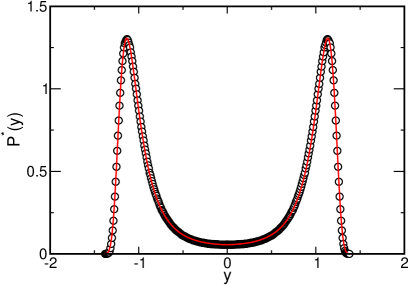
Figure 1: (Color online) The normalized distribution of the order parameter $P^{*}_{N}(y)$ (open circles) for $\Delta=0.2$ and $\sqrt{N}=18$, expressed as the function of the scaling variable $y=a_{m}^{-1}N^{\beta/(d\nu)}m$, at the packing fraction $\eta=0.5384$. The solid line is the universal function $P^{*}(y)$ for the Ising model [39]. The critical exponent $\nu$ is equal to 1, and $a_{m}$ is a proportionality constant.

$P^{*}_{N}(y)$ agrees very well with the universal distribution $P^{*}(y)$ for the value of $\eta$ that we identify with the apparent critical volume fraction $\eta_{\text{c}}^{*}(N)$. In the same way, we obtain apparent critical packing fractions for a set of systems with a different size. In figure 2, we present the plot of apparent critical densities for different system sizes calculated for the non-additivity parameter $\Delta=0.2$. The apparent critical packing fractions are estimated for a set of finite systems with $\sqrt{N}=\{18,20,22,24,26,28,30\}$. The critical packing fraction as a function of $N^{-1/2}$ for an infinite system was obtained by fitting the set of apparent critical packing fractions to a straight line and extrapolating the value of the critical packing fraction at infinity. The same procedure was used to determine the critical packing fractions for all the values of the non-additivity parameter $\Delta$.

In practice, the shape of the rescaled distribution function $P^{*}_{N}(y)$ is compared with the universal distribution of the order parameter, $P^{*}(y)$, for the first estimation of the apparent critical packing fraction. In order to determine the precise value of the apparent critical packing fraction, the fourth order cumulants,

$$U_{N}=1-\frac{\langle m^{4}\rangle}{3\langle m^{2}\rangle^{2}}\,.$$ (3.1)

are calculated for the values of the packing fraction $\eta$ for which the distribution functions are the most similar to the universal distribution $P^{*}(y)$. To calculate the matching point, the values of the cumulant $U_{N}(\eta)$ have been interpolated near the universal value $U_{N}^{*}$. We use the fourth order cumulant $U_{N}$ [40], because its value at a fixed point has been already calculated for the 2D Ising universality class.

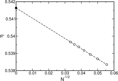
Figure 2: Scaling of the apparent critical packing fraction with the system size $\sqrt{N}=\{18,20,22,24,26,28,30\}$ for $\Delta=0.2$. The open circles represent the apparent critical packing fractions for different system sizes obtained by matching $P^{*}_{N}(y)$ with the universal function as in figure 1. The solid circle is the critical packing fraction for the infinite system [see equation (2.1)]. The dashed line is the least square fit of the apparent critical packing fractions to a straight line.

The $n$-th moment $\langle m^{n}\rangle$ can be easily calculated from the distribution of the order parameter $P_{N}(m)$:

$$\langle m^{n}\rangle=\frac{\sum_{m}m^{n}P_{N}(m)}{\sum_{m}P_{N}(m)}\,.$$ (3.2)

The apparent critical packing fractions $\eta_{\text{c}}^{*}(N)$ satisfy the equation $U_{N}(\eta_{\text{c}}^{*})=U^{*}$, and have been read off from the interpolated line for the value of $U^{*}=0.61069$ [41]. In figure 3, we present the cumulants, $U_{N}(m)$, as functions of the packing fraction for different system sizes $N$.

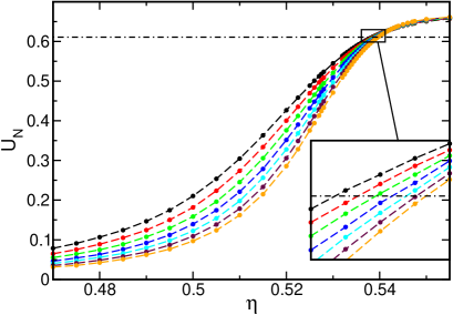
Figure 3: (Color online) Fourth order cumulant, $U_{N}(\eta)$, as a function of the packing fraction $\eta$ for the non-additivity parameter $\Delta=0.2$ and $\sqrt{N}=\{18,20,22,24,26,28,30\}$. The solid circles are the results of the simulations. The dashed line is just to guide the eye. The dash-dotted line is plotted at the universal value of the cumulant $U^{*}=0.61069$.

The curves cross at the values of the cumulant higher than the universal value $U^{*}$. Similar behavior was observed in references [20, 24].

In figure 4 we present the results of our calculation of the critical packing fractions for a set of the non-additivity parameter $\Delta$, compared with the results already reported in the literature. The calculations reported in reference [26] significantly overestimate and in reference [27] significantly underestimate the results of other works [20, 25, 13, 24]. This is most probably the result of inappropriate simulation methods employed in those calculations. It can be easily noticed that the results of our calculations are in very good agreement with the results of the calculations reported in reference [20] and reference [24]. In all these works, the authors use cluster algorithms in the simulations and the critical packing fractions are calculated for infinite systems where different kinds of finite size scaling analysis were used. In reference [25], the critical point packing fraction was obtained using the method of crossing the reduced second moment. This method is not as precise as the method of finite size scaling analysis. In reference [13], the critical packing fraction was estimated from the simulation of finite systems of the order of $N=2000$ molecules. Thus, the values of the critical packing fractions should be lower than the values of the critical packing fractions obtained for infinite systems.

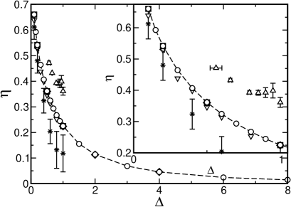
Figure 4: The critical packing fraction as a function of the non-additivity parameter $\Delta$. The open circles show the calculations from this work, the triangles up — reference [26], the stars — [27], the triangles down — [13], the squares — [24], the diamonds — [20], the triangle right-hand — [25]. The dashed line is just to guide the eye.

In our work, we employ the same cluster algorithm as in reference [24]. We use, however, a different numerical algorithm to identify the clusters, and different scaling procedure to obtain the critical packing fraction. In reference [20], a different cluster algorithm is used, where the clusters are built by superimposing two configurations and identifying the clusters by selecting the groups of overlapping molecules in the sense of hard core interactions. This method works very well for sufficiently large values of the non-additivity parameter $\Delta$ but is not as good for small $\Delta$. In reference [20], calculations were performed for $\Delta\in\{0.5,1.0,2.0,4.0\}$. The cluster algorithm used in reference [24] and in our calculations works very well for any value of the non-additivity parameters. In reference [24], calculations were performed for $\Delta\in\{0.1,0.2,0.5,1.0\}$. In this work, we have performed calculations for all the values of the non-additivity parameter $\Delta$ for which the simulation results already existed, and we have extended the calculation to additional large and small non-additivities. We have performed the calculation for $\Delta\in\{0.1,0.15,0.2,0.3,0.4,0.5,0.6,0.7,0.8,0.9,1.0,1.5,2.0,3.0,4.0,6.0,8.0\}$. The critical packing fractions for this set of parameters are presented in table 1.

Table 1: The critical packing fractions $\eta_{\text{c}}$ for infinite systems for different values of the non-additivity parameter $\Delta$.

$\Delta$	0.1	0.15	0.2	0.3	0.4	0.5
$\eta_{\text{c}}$	0.6607(30)	0.5928(20)	0.5416(30)	0.4644(30)	0.4069(30)	0.3615(40)
$\Delta$	0.6	0.7	0.8	0.9	1.0	1.5
$\eta_{\text{c}}$	0.3246(40)	0.2936(30)	0.2674(40)	0.2447(40)	0.2250(30)	0.1554(30)
$\Delta$	2.0	3.0	4.0	6.0	8.0
$\eta_{\text{c}}$	0.1140(40)	0.0686(30)	0.0455(30)	0.0241(20)	0.0148(20)

In figure 4, the results of our calculations are indistinguishable from the results of calculations in references [20] and [24]. An increase of the non-additivity parameter $\Delta$ results in a decrease of the critical packing fraction as shown in figure 4. In the mixture of non-additive hard disks, we have a competition between the entropy of mixing and the excluded volume effects. When the non-additivity parameter is large, the excluded volume effects are strong and the demixing process takes place at a lower packing fraction. When the non-additivity parameter is small, the entropy of mixing dominates and the demixing takes place at a higher packing fraction.

4 Summary and conclusions

We have calculated the critical packing fractions with high accuracy for the non-additive hard disks mixtures for a wide range of the non-additivity parameter. We have used Monte Carlo simulations with cluster algorithm which resulted in rejection-free moves. We have used finite size scaling analysis based on the universal distribution of the order parameter to determine the critical packing fraction for infinite systems. The results of our calculations agree very well with the results of the previous calculations where the finite size scaling analysis was used. The proposed simulation method allows for accurate and unambiguous determination of the critical packing fraction for any value of the non-additivity parameter $\Delta$. We hope that the results of our calculations will be the reference point for testing the results of approximate theories for hard disks systems. They should also allow one to compare the critical properties of the particles adsorbed at flat or at curved surfaces, and to determine in this way the effect of the curvature of the underlying surface on the critical properties of the adsorbed fluid mixture.

Ukrainian 0

Обчислення критичної точки для бiнарних сумiшей симетричних неадитивних твердих дискiв

В.Т. Гуздзь, А. Цях

             
Iнститут фiзичної хiмiї Польської академiї наук, Варшава, Польща

References

-
[1]
Góźdź W.T., Sokołowska Z., Sokołowski S., Z. Phys.
Chem., 1991, 173, No. 1, 95;
doi:10.1524/zpch.1991.173.Part_1.095. -
[2]
Bucior K., Patrykiejew A., Pizio O., Sokołowski S., Sokołowska Z.,
Mol. Phys., 2003, 101, No. 6, 721;
doi:10.1080/0026897021000021859. - [3] Duda Y., Pizio O., Sokołowski S., J. Phys. Chem. B, 2004, 108, No. 50, 19442; doi:10.1021/jp040340x.
- [4] Patrykiejew A., Sokołowski S., J. Phys. Chem. C, 2007, 111, No. 43, 15664; doi:10.1021/jp0728813.
- [5] Borówko M., Sokołowski S., Staszewski T., J. Phys. Chem. B, 2012, 116, No. 10, 3115; doi:10.1021/jp300114y.
- [6] Patrykiejew A., Sokołowski S., J. Chem. Phys., 2012, 136, No. 14, 144702; doi:10.1063/1.3699330.
-
[7]
Veatch S.L., Soubias O., Keller S.L., Gawrisch K., Proc. Natl. Acad. Sci. USA., 2007,
104, No. 45, 17650;
doi:10.1073/pnas.0703513104. -
[8]
Honerkamp-Smith A.R., Veatch S.L., Keller S.L., Biochim. Biophys. Acta, 2009,
1788, No. 1, 53;
doi:10.1016/j.bbamem.2008.09.010. - [9] Góźdź W.T., Bobrovska N., Ciach A., J. Chem. Phys., 2012, 137, No. 1, 015101; doi:10.1063/1.4731646.
- [10] Góźdź W.T., Hołyst R., Phys. Rev. E, 1996, 54, No. 5, 5012; doi:10.1103/PhysRevE.54.5012.
- [11] Dotera T., Kimoto M., Matsuzawa J., Interface Focus, 2012, 2, No. 5, 575; doi:10.1098/rsfs.2011.0092.
- [12] Onsager L., Phys. Rev., 1944, 65, 117; doi:10.1103/PhysRev.65.117.
- [13] Fiumara G., Pandaram O.D., Pellicane G., Saija F., J. Chem. Phys., 2014, 141, No. 21, 214508; doi:10.1063/1.4902440.
- [14] Amar J.G., Mol. Phys., 1989, 67, 739; doi:10.1080/00268978900101411.
- [15] Lomba E., Alvarez M., Lee L., Almarza N., J. Chem. Phys., 1996, 104, 4180; doi:10.1063/1.471229.
-
[16]
Johnson G., Gould H., Machta J., Chayes L., Phys. Rev. Lett., 1997,
79, No. 14, 2612;
doi:10.1103/PhysRevLett.79.2612. - [17] Saija F., Pastore G., Giaquinta P.V., J. Phys. Chem. B, 1998, 102, No. 50, 10368; doi:10.1021/jp982202b.
- [18] Góźdź W.T., Pol. J. Chem., 2001, 75, No. 4, 517.
- [19] Góźdź W.T., J. Chem. Phys., 2003, 119, No. 6, 3309; doi:10.1063/1.1589746.
- [20] Buhot A., J. Chem. Phys., 2005, 122, No. 2, 024105; doi:10.1063/1.1831274.
- [21] Pellicane G., Pandaram O.D., J. Chem. Phys., 2014, 141, No. 4, 044508; doi:10.1063/1.4890742.
- [22] Góźdź W.T., J. Chem. Phys., 2005, 122, No. 7, 074505; doi:10.1063/1.1844332.
- [23] De Sanctis Lucentini P.G., Pellicane G., Phys. Rev. Lett., 2008, 101, 246101; doi:10.1103/PhysRevLett.101.246101.
- [24] Almarza N.G., Martín C., Lomba E., Bores C., J. Chem. Phys., 2015, 142, No. 1, 014702; doi:10.1063/1.4905273.
- [25] Muñoz-Salazar L., Odriozola G., Mol. Simul., 2010, 36, No. 3, 175; doi:10.1080/08927020903141027.
- [26] Nielaba P., Int. J. Thermophys., 1996, 17, No. 1, 157; doi:10.1007/BF01448218.
- [27] Saija F., Giaquinta P.V., J. Chem. Phys., 2002, 117, No. 12, 5780; doi:10.1063/1.1501126.
- [28] Góźdź W.T., Gubbins K.E., Panagiotopoulos A.Z., Mol. Phys., 1995, 84, No. 5, 825; doi:10.1080/00268979500100581.
- [29] Kofke D.A., Glandt E.D., Mol. Phys., 1988, 64, 1105; doi:10.1080/00268978800100743.
- [30] Metropolis N., Ulam S.M., J. Am. Stat. Assoc., 1949, 44, No. 247, 335; doi:10.1080/01621459.1949.10483310.
- [31] Metropolis N., Rosenbluth A.W., Rosenbluth M.N., Teller A.H., Teller E., J. Chem. Phys., 1953, 21, No. 6, 1087; doi:10.1063/1.1699114.
- [32] Florek K., Łukaszewicz J., Perkal J., Steinhaus H., Zubrzycki S., Colloquium Math., 1951, 2, No. 3–4, 282.
- [33] Florek K., Łukaszewicz J., Perkal J., Steinhaus H., Zubrzycki S., Przegl. Antrop., 1951, 17, 193.
- [34] Sibson R., Comput. J., 1973, 16, No. 1, 30; doi:10.1093/comjnl/16.1.30.
- [35] Fisher M.E., Barber M.N., Phys. Rev. Lett., 1972, 23, 1516; doi:10.1103/PhysRevLett.28.1516.
- [36] Phase Transitions and Critical Phenomena, 8th Edn., Domb C., Lebowitz J. (Eds.), Academic Press, London, 1983.
- [37] Wilding N.B., Phys. Rev. E, 1995, 52, 602; doi:10.1103/PhysRevE.52.602.
- [38] Nicolaides D., Bruce A.D., J. Phys. A: Math. Gen., 1988, 21, No. 1, 233; doi:10.1088/0305-4470/21/1/028.
- [39] Liu Y., Panagiotopoulos A.Z., Debenedetti P.G., J. Chem. Phys., 2010, 132, No. 14, 144107; doi:10.1063/1.3377089.
- [40] Binder K., Phys. Rev. Lett., 1981, 47, 693; doi:10.1103/PhysRevLett.47.693.
- [41] Kamieniarz G., Blote H.W.J., J. Phys. A: Math. Gen., 1993, 26, No. 2, 201; doi:10.1088/0305-4470/26/2/009.
Ukrainian \adddialect\l@ukrainian0 \l@ukrainian